Understanding and implementing the GPT-1, GPT-2 and GPT-3 architectures
Originally appeared here:
Meet GPT, The Decoder-Only Transformer
Go Here to Read this Fast! Meet GPT, The Decoder-Only Transformer
Understanding and implementing the GPT-1, GPT-2 and GPT-3 architectures
Originally appeared here:
Meet GPT, The Decoder-Only Transformer
Go Here to Read this Fast! Meet GPT, The Decoder-Only Transformer


When you’re deep in rapid prototyping, it’s tempting to skip clean scoping or reuse common variable names (hello, df!), thinking it will save time. But this can lead to sneaky bugs that break your workflow.
The good news? Writing clean, well-scoped code does not require additional effort once you understand the basic principles.
Let’s break it down.
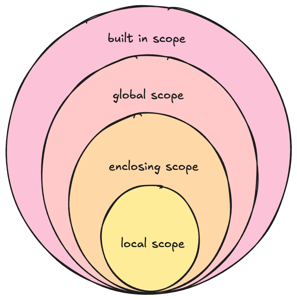
Think of a variable as a container that will store some information. Scope refers to the region of your code where a variable is accessible.
Scope prevents accidental changes by limiting where variables can be read or modified. If every variable was accessible from anywhere, you’ll have to keep track of all of them to avoid overwriting it accidentally.
In Python, scope is defined by the LEGB rule, which stands for: local, enclosing, global and built-in.
Let’s illustrate this with an example.
# Global scope, 7% tax
default_tax = 0.07

def calculate_invoice(price):
    # Enclosing scope
    discount = 0.10
    total_after_discount = 0

    def apply_discount():
        nonlocal total_after_discount

        # Local scope
        tax = price * default_tax
        total_after_discount = price - (price * discount)
        return total_after_discount + tax

    final_price = apply_discount()
    return final_price, total_after_discount

# Built-in scope
print("Invoice total:", round(calculate_invoice(100)[0], 2))
Variables inside a function are in the local scope. They can only be accessed within that function.
In the example, tax is a local variable inside apply_discount. It is not accessible outside this function.
These refer to variables in a function that contains a nested function. These variables are not global but can be accessed by the inner (nested) function. In this example, discount and total_after_discount are variables in the enclosing scope of apply_discount .
The nonlocal keyword:
The nonlocal keyword is used to modify variables in the enclosing scope, not just read them.
For example, suppose you want to update the variable total_after_discount, which is in the enclosing scope of the function. Without nonlocal, if you assign to total_after_discount inside the inner function, Python will treat it as a new local variable, effectively shadowing the outer variable. This can introduce bugs and unexpected behavior.
Variables that are defined outside all functions and accessible throughout.
The global statement
When you declare a variable as global inside a function, Python treats it as a reference to the variable outside the function. This means that changes to it will affect the variable in the global scope.
With the global keyword, Python will create a new local variable.
x = 10  # Global variable

def modify_global():
    global x  # Declare that x refers to the global variable
    x = 20    # Modify the global variable

modify_global()
print(x)  # Output: 20. If "global" was not declared, this would read 10
Refers to the reserved keywords that Python uses for it’s built-in functions, such as print , def , round and so on. This can be accessed at any level.
Both keywords are crucial for modifying variables in different scopes, but they’re used differently.
Variable shadowing happens when a variable in an inner scope hides a variable from an outer scope.
Within the inner scope, all references to the variable will point to the inner variable, not the outer one. This can lead to confusion and unexpected outputs if you’re not careful.
Once execution returns to the outer scope, the inner variable ceases to exist, and any reference to the variable will point back to the outer scope variable.
Here’s a quick example. x is shadowed in each scope, resulting in different outputs depending on the context.
#global scope
x = 10

def outer_function():
    #enclosing scope
    x = 20

    def inner_function():
        #local scope
        x = 30
        print(x)  # Outputs 30

    inner_function()
    print(x)  # Outputs 20

outer_function()
print(x)  # Outputs 10
A similar concept to variable shadowing, but this occurs when a local variable redefines or overwrites a parameter passed to a function.
def foo(x):
    x = 5  # Shadows the parameter `x`
    return x

foo(10)  # Output: 5
x is passed as 10. But it is immediately shadowed and overwritten by x=5
Each recursive call gets its own execution context, meaning that the local variables and parameters in that call are independent of previous calls.
However, if a variable is modified globally or passed down explicitly as a parameter, the change can influence subsequent recursive calls.
Let’s illustrate this with an example.
counter = 0  # Global variable

def count_up(n):
    global counter
    if n > 0:
        counter += 1
        count_up(n - 1)

count_up(5)
print(counter)  # Output: 5
counter is a global variable shared across all recursive calls. It gets incremented at each level of recursion, and its final value (5) is printed after the recursion completes.
def count_up(n, counter=0):
    if n > 0:
        counter += 1
        return count_up(n - 1, counter)
    return counter

result = count_up(5)
print(result)  # Output: 5
Avoid vague names like df or x. Use descriptive names such as customer_sales_df or sales_records_df for clarity.
This is the standard naming convention for constants in Python. For example, MAX_RETRIES = 5.
Global variables introduces bugs and makes code harder to test and maintain. It’s best to pass variables explicitly between functions.
What’s a pure function?
Using nonlocal or global would make the function impure.
However, if you’re working with a closure, you should use the nonlocal keyword to modify variables in the enclosing (outer) scope, which helps prevent variable shadowing.
A closure occurs when a nested function (inner function) captures and refers to variables from its enclosing function (outer function). This allows the inner function to “remember” the environment in which it was created, including access to variables from the outer function’s scope, even after the outer function has finished executing.
The concept of closures can go really deep, so tell me in the comments if this is something I should dive into in the next article! 🙂
If you need to refer to an outer variable, avoid reusing its name in an inner scope. Use distinct names to clearly distinguish the variables.
That’s a wrap! Thanks for sticking with me till the end.
Have you encountered any of these challenges in your own work? Drop your thoughts in the comments below!
I write regularly on Python, software development and the projects I build, so give me a follow to not miss out. See you in the next article 🙂
Why Variable Scoping Can Make or Break Your Data Science Workflow was originally published in Towards Data Science on Medium, where people are continuing the conversation by highlighting and responding to this story.
Originally appeared here:
Why Variable Scoping Can Make or Break Your Data Science Workflow
Go Here to Read this Fast! Why Variable Scoping Can Make or Break Your Data Science Workflow
Is C is faster than Rust? I had always assumed the answer to that question to be yes, but I recently felt the need to test my assumptions.
Originally appeared here:
Measuring The Execution Times of C Versus Rust
Go Here to Read this Fast! Measuring The Execution Times of C Versus Rust


Suppressing Logical Errors Exponentially! For the First Time
Originally appeared here:
Google’s Willow Quantum Computing Chip: A Game Changer?
Go Here to Read this Fast! Google’s Willow Quantum Computing Chip: A Game Changer?
Illustrated with an example of Multimodal offline batch inference with CLIP
Originally appeared here:
Distributed Parallel Computing Made Easy with Ray
Go Here to Read this Fast! Distributed Parallel Computing Made Easy with Ray

This article describes the architecture and design of a Home Assistant (HA) integration called home-generative-agent. This project uses LangChain and LangGraph to create a generative AI agent that interacts with and automates tasks within a HA smart home environment. The agent understands your home’s context, learns your preferences, and interacts with you and your home to accomplish activities you find valuable. Key features include creating automations, analyzing images, and managing home states using various LLMs (Large Language Models). The architecture involves both cloud-based and edge-based models for optimal performance and cost-effectiveness. Installation instructions, configuration details, and information on the project’s architecture and the different models used are included and can be found on the home-generative-agent GitHub. The project is open-source and welcomes contributions.
These are some of the features currently supported:
This is my personal project and an example of what I call learning-directed hacking. The project is not affiliated with my work at Amazon nor am I associated with the organizations responsible for Home Assistant or LangChain/LangGraph in any way.
Creating an agent to monitor and control your home can lead to unexpected actions and potentially put your home and yourself at risk due to LLM hallucinations and privacy concerns, especially when exposing home states and user information to cloud-based LLMs. I have made reasonable architectural and design choices to mitigate these risks, but they cannot be completely eliminated.
One key early decision was to rely on a hybrid cloud-edge approach. This enables the use of the most sophisticated reasoning and planning models available, which should help reduce hallucinations. Simpler, more task-focused edge models are employed to further minimize LLM errors.
Another critical decision was to leverage LangChain’s capabilities, which allow sensitive information to be hidden from LLM tools and provided only at runtime. For instance, tool logic may require using the ID of the user who made a request. However, such values should generally not be controlled by the LLM. Allowing the LLM to manipulate the user ID could pose security and privacy risks. To mitigate this, I utilized the InjectedToolArg annotation.
Additionally, using large cloud-based LLMs incurs significant cloud costs, and the edge hardware required to run LLM edge models can be expensive. The combined operational and installation costs are likely prohibitive for the average user at this time. An industry-wide effort to “make LLMs as cheap as CNNs” is needed to bring home agents to the mass market.
It is important to be aware of these risks and understand that, despite these mitigations, we are still in the early stages of this project and home agents in general. Significant work remains to make these agents truly useful and trustworthy assistants.
Below is a high-level view of the home-generative-agent architecture.
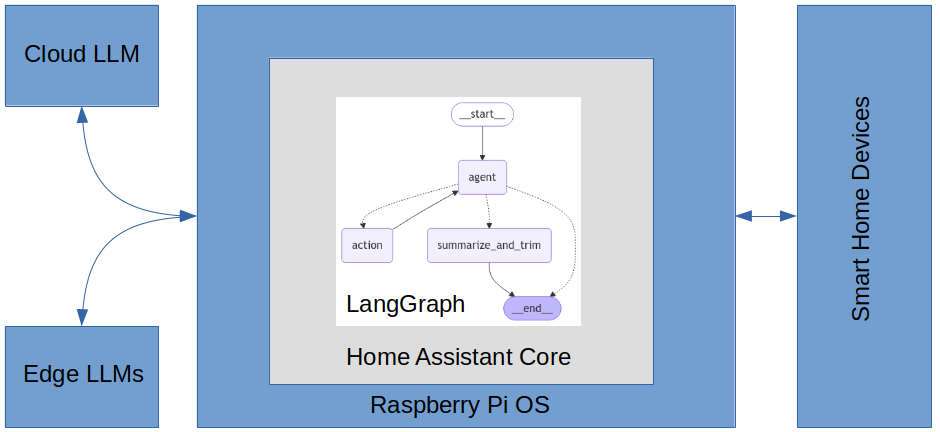
The general integration architecture follows the best practices as described in Home Assistant Core and is compliant with Home Assistant Community Store (HACS) publishing requirements.
The agent is built using LangGraph and uses the HA conversation component to interact with the user. The agent uses the Home Assistant LLM API to fetch the state of the home and understand the HA native tools it has at its disposal. I implemented all other tools available to the agent using LangChain. The agent employs several LLMs, a large and very accurate primary model for high-level reasoning, smaller specialized helper models for camera image analysis, primary model context summarization, and embedding generation for long-term semantic search. The primary model is cloud-based, and the helper models are edge-based and run under the Ollama framework on a computer located in the home.
The models currently being used are summarized below.
LangGraph powers the conversation agent, enabling you to create stateful, multi-actor applications utilizing LLMs as quickly as possible. It extends LangChain’s capabilities, introducing the ability to create and manage cyclical graphs essential for developing complex agent runtimes. A graph models the agent workflow, as seen in the image below.
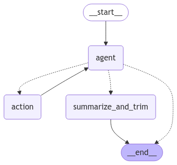
The agent workflow has five nodes, each Python module modifying the agent’s state, a shared data structure. The edges between the nodes represent the allowed transitions between them, with solid lines unconditional and dashed lines conditional. Nodes do the work, and edges tell what to do next.
The __start__ and __end__ nodes inform the graph where to start and stop. The agent node runs the primary LLM, and if it decides to use a tool, the action node runs the tool and then returns control to the agent. The summarize_and_trim node processes the LLM’s context to manage growth while maintaining accuracy if agent has no tool to call and the number of messages meets the below-mentioned conditions.
You need to carefully manage the context length of LLMs to balance cost, accuracy, and latency and avoid triggering rate limits such as OpenAI’s Tokens per Minute restriction. The system controls the context length of the primary model in two ways: it trims the messages in the context if they exceed a max parameter, and the context is summarized once the number of messages exceeds another parameter. These parameters are configurable in const.py; their description is below.
The summarize_and_trim node in the graph will trim the messages only after content summarization. You can see the Python code associated with this node in the snippet below.
async def _summarize_and_trim(
        state: State, config: RunnableConfig, *, store: BaseStore
    ) -> dict[str, list[AnyMessage]]:
    """Coroutine to summarize and trim message history."""
    summary = state.get("summary", "")

    if summary:
        summary_message = SUMMARY_PROMPT_TEMPLATE.format(summary=summary)
    else:
        summary_message = SUMMARY_INITIAL_PROMPT

    messages = (
        [SystemMessage(content=SUMMARY_SYSTEM_PROMPT)] +
        state["messages"] +
        [HumanMessage(content=summary_message)]
    )

    model = config["configurable"]["vlm_model"]
    options = config["configurable"]["options"]
    model_with_config = model.with_config(
        config={
            "model": options.get(
                CONF_VLM,
                RECOMMENDED_VLM,
            ),
            "temperature": options.get(
                CONF_SUMMARIZATION_MODEL_TEMPERATURE,
                RECOMMENDED_SUMMARIZATION_MODEL_TEMPERATURE,
            ),
            "top_p": options.get(
                CONF_SUMMARIZATION_MODEL_TOP_P,
                RECOMMENDED_SUMMARIZATION_MODEL_TOP_P,
            ),
            "num_predict": VLM_NUM_PREDICT,
        }
    )

    LOGGER.debug("Summary messages: %s", messages)
    response = await model_with_config.ainvoke(messages)

    # Trim message history to manage context window length.
    trimmed_messages = trim_messages(
        messages=state["messages"],
        token_counter=len,
        max_tokens=CONTEXT_MAX_MESSAGES,
        strategy="last",
        start_on="human",
        include_system=True,
    )
    messages_to_remove = [m for m in state["messages"] if m not in trimmed_messages]
    LOGGER.debug("Messages to remove: %s", messages_to_remove)
    remove_messages = [RemoveMessage(id=m.id) for m in messages_to_remove]

    return {"summary": response.content, "messages": remove_messages}
The latency between user requests or the agent taking timely action on the user’s behalf is critical for you to consider in the design. I used several techniques to reduce latency, including using specialized, smaller helper LLMs running on the edge and facilitating primary model prompt caching by structuring the prompts to put static content, such as instructions and examples, upfront and variable content, such as user-specific information at the end. These techniques also reduce primary model usage costs considerably.
You can see the typical latency performance below.
The agent can use HA tools as specified in the LLM API and other tools built in the LangChain framework as defined in tools.py. Additionally, you can extend the LLM API with tools of your own as well. The code gives the primary LLM the list of tools it can call, along with instructions on using them in its system message and in the docstring of the tool’s Python function definition. You can see an example of docstring instructions in the code snippet below for the get_and_analyze_camera_image tool.
@tool(parse_docstring=False)
async def get_and_analyze_camera_image( # noqa: D417
        camera_name: str,
        detection_keywords: list[str] | None = None,
        *,
        # Hide these arguments from the model.
        config: Annotated[RunnableConfig, InjectedToolArg()],
    ) -> str:
    """
    Get a camera image and perform scene analysis on it.

    Args:
        camera_name: Name of the camera for scene analysis.
        detection_keywords: Specific objects to look for in image, if any.
            For example, If user says "check the front porch camera for
            boxes and dogs", detection_keywords would be ["boxes", "dogs"].

    """
    hass = config["configurable"]["hass"]
    vlm_model = config["configurable"]["vlm_model"]
    options = config["configurable"]["options"]
    image = await _get_camera_image(hass, camera_name)
    return await _analyze_image(vlm_model, options, image, detection_keywords)
If the agent decides to use a tool, the LangGraph node action is entered, and the node’s code runs the tool. The node uses a simple error recovery mechanism that will ask the agent to try calling the tool again with corrected parameters in the event of making a mistake. The code snippet below shows the Python code associated with the action node.
async def _call_tools(
        state: State, config: RunnableConfig, *, store: BaseStore
    ) -> dict[str, list[ToolMessage]]:
    """Coroutine to call Home Assistant or langchain LLM tools."""
    # Tool calls will be the last message in state.
    tool_calls = state["messages"][-1].tool_calls

    langchain_tools = config["configurable"]["langchain_tools"]
    ha_llm_api = config["configurable"]["ha_llm_api"]

    tool_responses: list[ToolMessage] = []
    for tool_call in tool_calls:
        tool_name = tool_call["name"]
        tool_args = tool_call["args"]

        LOGGER.debug(
            "Tool call: %s(%s)", tool_name, tool_args
        )

        def _handle_tool_error(err:str, name:str, tid:str) -> ToolMessage:
            return ToolMessage(
                content=TOOL_CALL_ERROR_TEMPLATE.format(error=err),
                name=name,
                tool_call_id=tid,
                status="error",
            )

        # A langchain tool was called.
        if tool_name in langchain_tools:
            lc_tool = langchain_tools[tool_name.lower()]

            # Provide hidden args to tool at runtime.
            tool_call_copy = copy.deepcopy(tool_call)
            tool_call_copy["args"].update(
                {
                    "store": store,
                    "config": config,
                }
            )

            try:
                tool_response = await lc_tool.ainvoke(tool_call_copy)
            except (HomeAssistantError, ValidationError) as e:
                tool_response = _handle_tool_error(repr(e), tool_name, tool_call["id"])
        # A Home Assistant tool was called.
        else:
            tool_input = llm.ToolInput(
                tool_name=tool_name,
                tool_args=tool_args,
            )

            try:
                response = await ha_llm_api.async_call_tool(tool_input)

                tool_response = ToolMessage(
                    content=json.dumps(response),
                    tool_call_id=tool_call["id"],
                    name=tool_name,
                )
            except (HomeAssistantError, vol.Invalid) as e:
                tool_response = _handle_tool_error(repr(e), tool_name, tool_call["id"])

        LOGGER.debug("Tool response: %s", tool_response)
        tool_responses.append(tool_response)
    return {"messages": tool_responses}
The LLM API instructs the agent always to call tools using HA built-in intents when controlling Home Assistant and to use the intents `HassTurnOn` to lock and `HassTurnOff` to unlock a lock. An intent describes a user’s intention generated by user actions.
You can see the list of LangChain tools that the agent can use below.
I built the HA installation on a Raspberry Pi 5 with SSD storage, Zigbee, and LAN connectivity. I deployed the edge models under Ollama on an Ubuntu-based server with an AMD 64-bit 3.4 GHz CPU, Nvidia 3090 GPU, and 64 GB system RAM. The server is on the same LAN as the Raspberry Pi.
I’ve been using this project at home for a few weeks and have found it useful but frustrating in a few areas that I will be working on to address. Below is a list of pros and cons of my experience with the agent.
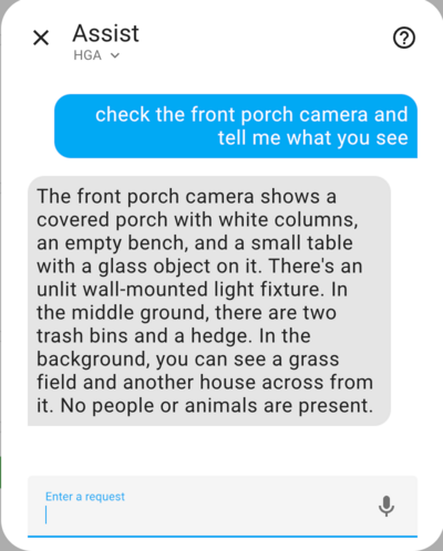
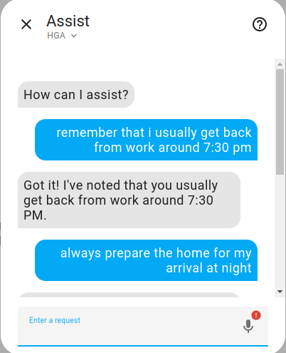
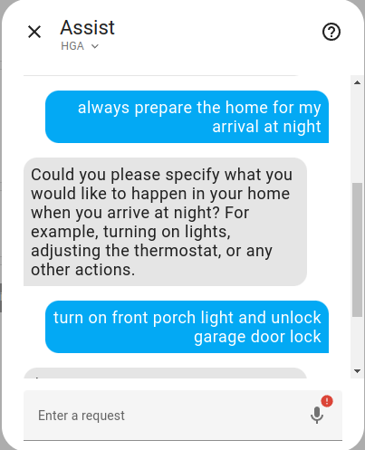
Here are a few examples of what you can do with the home-generative-agent (HGA) integration as illustrated by screenshots of the Assist dialog taken by me during interactions with my HA installation.
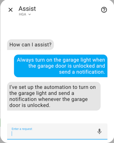
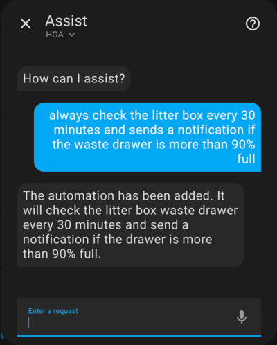
The snippet below shows that the agent is fluent in YAML based on what it generated and registered as an HA automation.
alias: Check Litter Box Waste Drawer
triggers:
  - minutes: /30
    trigger: time_pattern
conditions:
  - condition: numeric_state
    entity_id: sensor.litter_robot_4_waste_drawer
    above: 90
actions:
  - data:
      message: The Litter Box waste drawer is more than 90% full!
    action: notify.notify
https://github.com/user-attachments/assets/230baae5-8702-4375-a3f0-ffa981ee66a3
https://github.com/user-attachments/assets/96f834a8-58cc-4bd9-a899-4604c1103a98
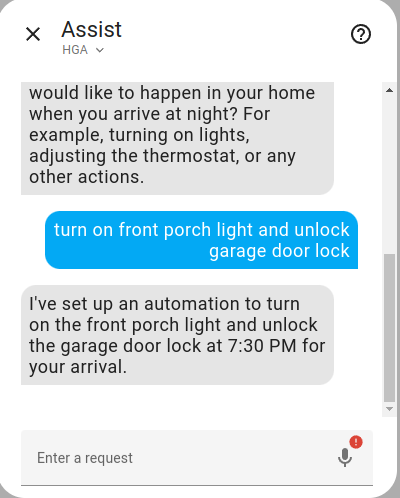
You can see that the agent correctly generates the automation below.
alias: Prepare Home for Arrival
description: Turn on front porch light and unlock garage door lock at 7:30 PM
mode: single
triggers:
 - at: "19:30:00"
    trigger: time
actions:
  - target:
      entity_id: light.front_porch_light
    action: light.turn_on
    data: {}
  - target:
      entity_id: lock.garage_door_lock
    action: lock.unlock
    data: {}
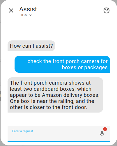
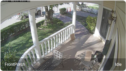
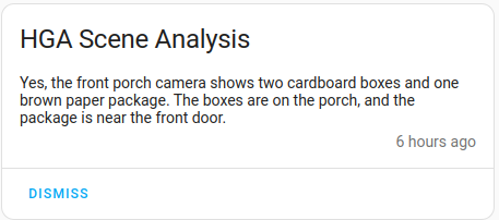
Below is the camera image the agent analyzed, you can see that two packages are visible.
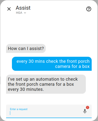
Below is an example notification from this automation if any boxes or packages are visible.
The Home Generative Agent offers an intriguing way to make your Home Assistant setup more user-friendly and intuitive. By enabling natural language interactions and simplifying automation, it provides a practical and useful tool for everyday smart home use.
Using a home generative agent carries security, privacy and cost risks that need further mitigation and innovation before it can be truly useful for the mass market.
Whether you’re new to Home Assistant or a seasoned user, this integration is a great way to enhance your system’s capabilities and get familiar with using generative AI and agents at home. If you’re interested in exploring its potential, visit the Home Generative Agent GitHub page and get started today.
1. Using the tool of choice, open your HA configuration’s directory (folder) (where you find configuration.yaml).
2. If you do not have a `custom_components` directory (folder), you must create it.
3. In the custom_components directory (folder), create a new folder called home_generative_agent.
4. Download _all_ the files from the custom_components/home_generative_agent/ directory (folder) in this repository.
4. Place the files you downloaded in the new directory (folder) you created.
6. Restart Home Assistant
7. In the HA UI, go to “Configuration” -> “Integrations” click “+,” and search for “Home Generative Agent”
Configuration is done in the HA UI and via the parameters in const.py.
LangChain Meets Home Assistant: Unlock the Power of Generative AI in Your Smart Home was originally published in Towards Data Science on Medium, where people are continuing the conversation by highlighting and responding to this story.
Originally appeared here:
LangChain Meets Home Assistant: Unlock the Power of Generative AI in Your Smart Home


Is there ever a good reason for starting a bar chart above zero?
Originally appeared here:
Awesome Plotly with Code Series (Part 7): Cropping the y-axis in Bar Charts


Just like Mr. Miyagi taught young Daniel LaRusso karate through repetitive simple chores, which ultimately transformed him into the Karate Kid, mastering foundational algorithms like linear regression lays the groundwork for understanding the most complex of AI architectures such as Deep Neural Networks and LLMs.
Through this deep dive into the simple yet powerful linear regression, you will learn many of the fundamental parts that make up the most advanced models built today by billion-dollar companies.
Linear regression is a simple mathematical method used to understand the relationship between two variables and make predictions. Given some data points, such as the one below, linear regression attempts to draw the line of best fit through these points. It’s the “wax on, wax off” of data science.
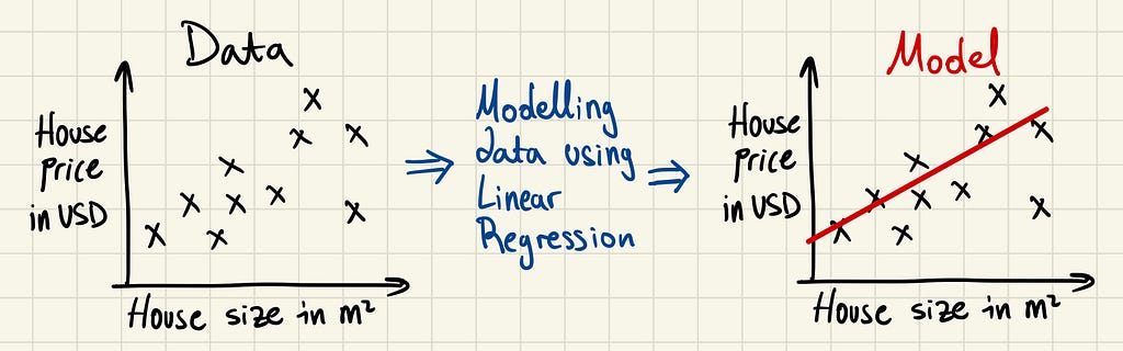
Once this line is drawn, we have a model that we can use to predict new values. In the above example, given a new house size, we could attempt to predict its price with the linear regression model.

Y is the dependent variable, that which you want to calculate — the house price in the previous example. Its value depends on other variables, hence its name.
X are the independent variables. These are the factors that influence the value of Y. When modelling, the independent variables are the input to the model, and what the model spits out is the prediction or Ŷ.
β are parameters. We give the name parameter to those values that the model adjusts (or learns) to capture the relationship between the independent variables X and the dependent variable Y. So, as the model is trained, the input of the model will remain the same, but the parameters will be adjusted to better predict the desired output.
We require a few things to be able to adjust the parameters and achieve accurate predictions.
Let’s go over a cost function and training algorithm that can be used in linear regression.
MSE is a commonly used cost function in regression problems, where the goal is to predict a continuous value. This is different from classification tasks, such as predicting the next token in a vocabulary, as in Large Language Models. MSE focuses on numerical differences and is used in a variety of regression and neural network problems, this is how you calculate it:

You will notice that as our prediction gets closer to the target value the MSE gets lower, and the further away they are the larger it grows. Both ways progress quadratically because the difference is squared.
The concept of gradient descent is that we can travel through the “cost space” in small steps, with the objective of arriving at the global minimum — the lowest value in the space. The cost function evaluates how well the current model parameters predict the target by giving us the loss value. Randomly modifying the parameters does not guarantee any improvements. But, if we examine the gradient of the loss function with respect to each parameter, i.e. the direction of the loss after an update of the parameter, we can adjust the parameters to move towards a lower loss, indicating that our predictions are getting closer to the target values.
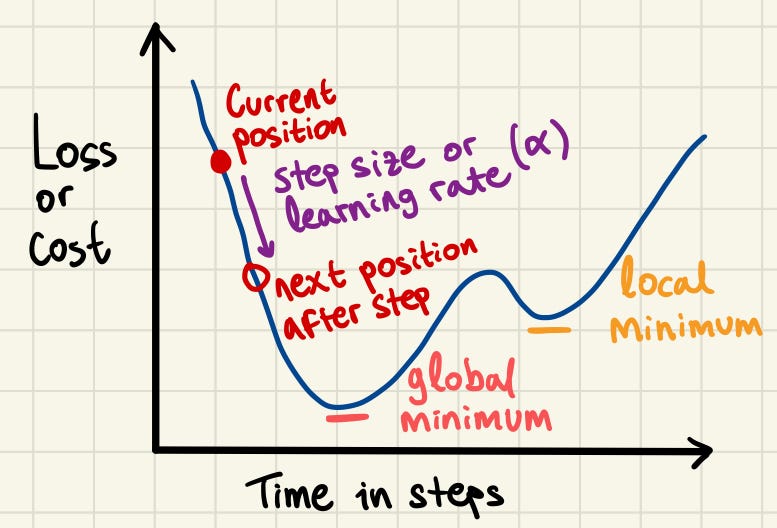
The steps in gradient descent must be carefully sized to balance progress and precision. If the steps are too large, we risk overshooting the global minimum and missing it entirely. On the other hand, if the steps are too small, the updates will become inefficient and time-consuming, increasing the likelihood of getting stuck in a local minimum instead of reaching the desired global minimum.

In the context of linear regression, θ could be β0 or β1. The gradient is the partial derivative of the cost function with respect to θ, or in simpler terms, it is a measure of how much the cost function changes when the parameter θ is slightly adjusted.
A large gradient indicates that the parameter has a significant effect on the cost function, while a small gradient suggests a minor effect. The sign of the gradient indicates the direction of change for the cost function. A negative gradient means the cost function will decrease as the parameter increases, while a positive gradient means it will increase.
So, in the case of a large negative gradient, what happens to the parameter? Well, the negative sign in front of the learning rate will cancel with the negative sign of the gradient, resulting in an addition to the parameter. And since the gradient is large we will be adding a large number to it. So, the parameter is adjusted substantially reflecting its greater influence on reducing the cost function.
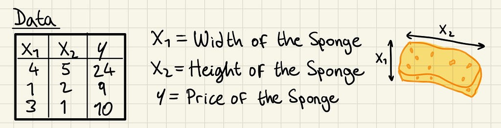
Let’s take a look at the prices of the sponges Karate Kid used to wash Mr. Miyagi’s car. If we wanted to predict their price (dependent variable) based on their height and width (independent variables), we could model it using linear regression.
We can start with these three training data samples.
Now, let’s use the Mean Square Error (MSE) as our cost function J, and linear regression as our model.
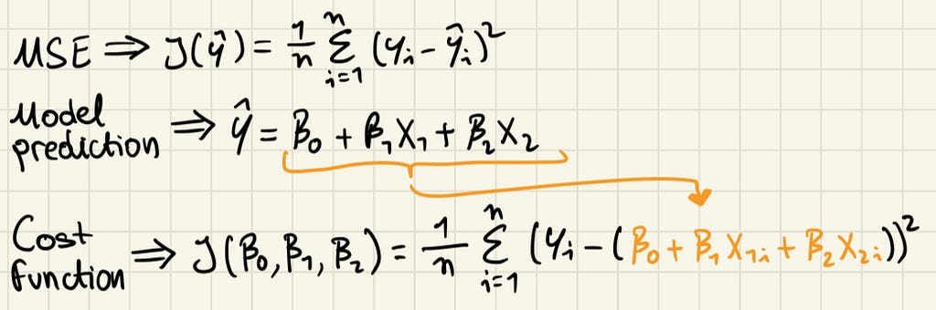
The linear regression formula uses X1 and X2 for width and height respectively, notice there are no more independent variables since our training data doesn’t include more. That is the assumption we take in this example, that the width and height of the sponge are enough to predict its price.
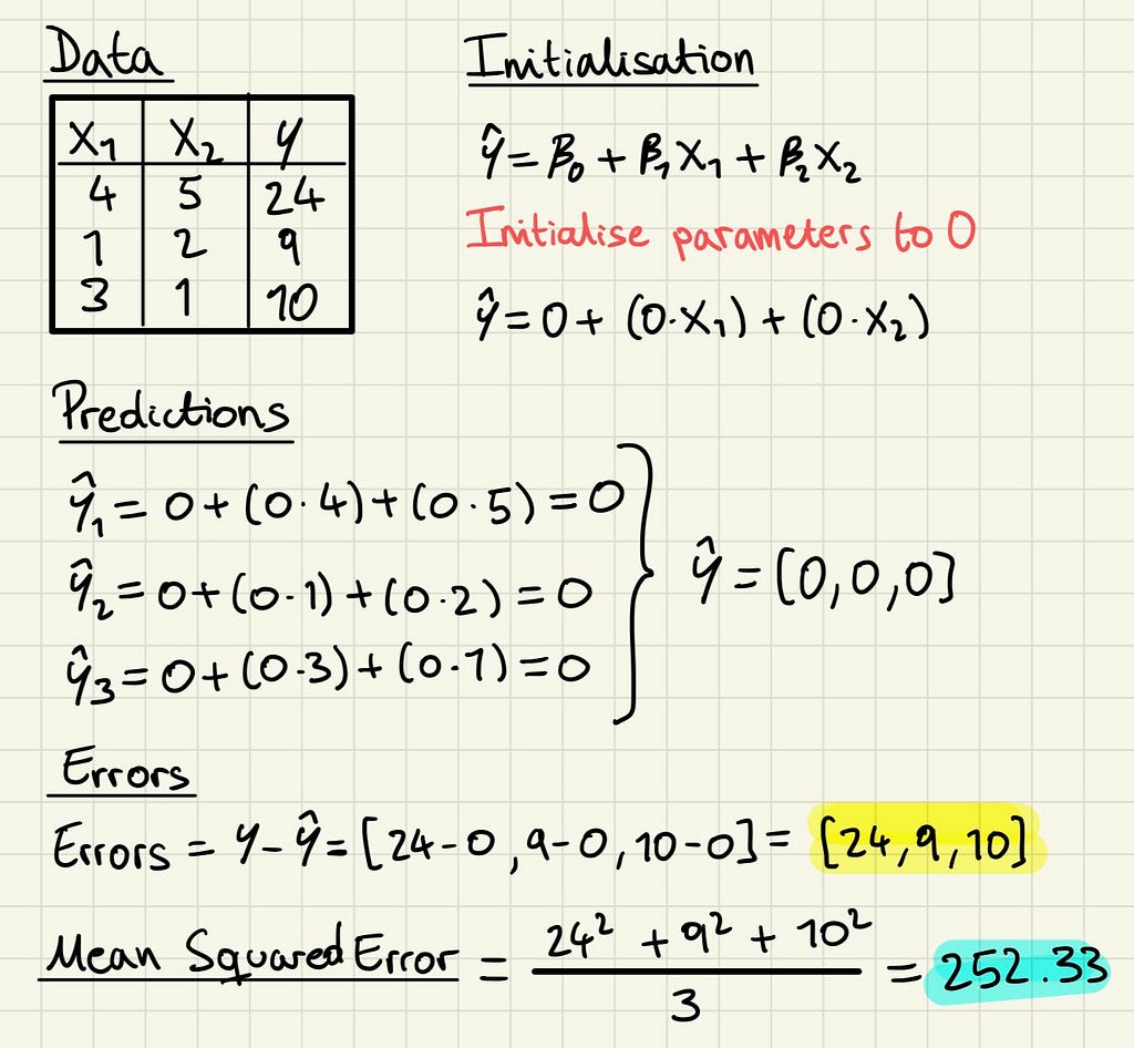
Now, the first step is to initialise the parameters, in this case to 0. We can then feed the independent variables into the model to get our predictions, Ŷ, and check how far these are from our target Y.
Right now, as you can imagine, the parameters are not very helpful. But we are now prepared to use the Gradient Descent algorithm to update the parameters into more useful ones. First, we need to calculate the partial derivatives of each parameter, which will require some calculus, but luckily we only need to this once in the whole process.
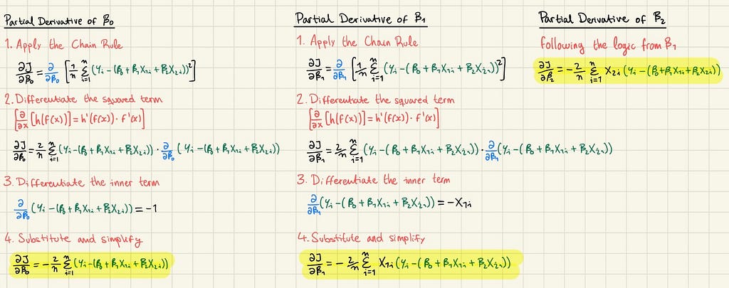
With the partial derivatives, we can substitute in the values from our errors to calculate the gradient of each parameter.
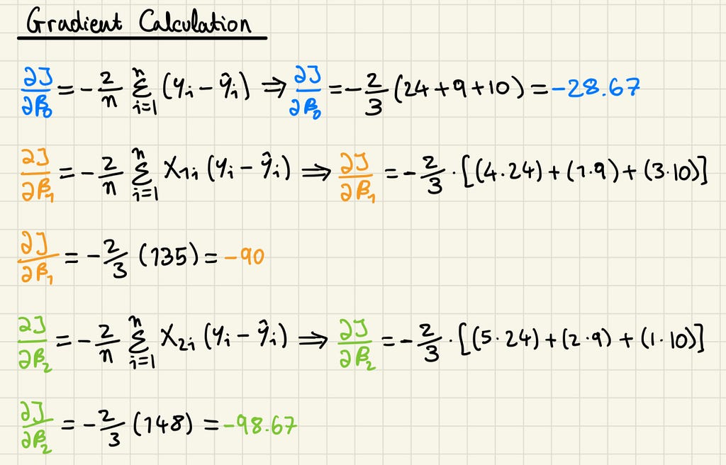
Notice there wasn’t any need to calculate the MSE, as it’s not directly used in the process of updating parameters, only its derivative is. It’s also immediately apparent that all gradients are negative, meaning that all can be increased to reduce the cost function. The next step is to update the parameters with a learning rate, which is a hyper-parameter, i.e. a configuration setting in a machine learning model that is specified before the training process begins. Unlike model parameters, which are learned during training, hyper-parameters are set manually and control aspects of the learning process. Here we arbitrarily use 0.01.
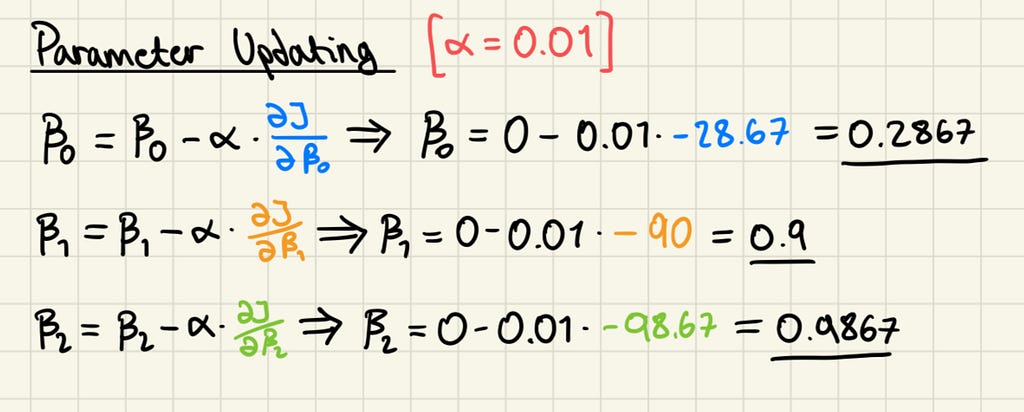
This has been the final step of our first iteration in the process of gradient descent. We can use these new parameter values to make new predictions and recalculate the MSE of our model.
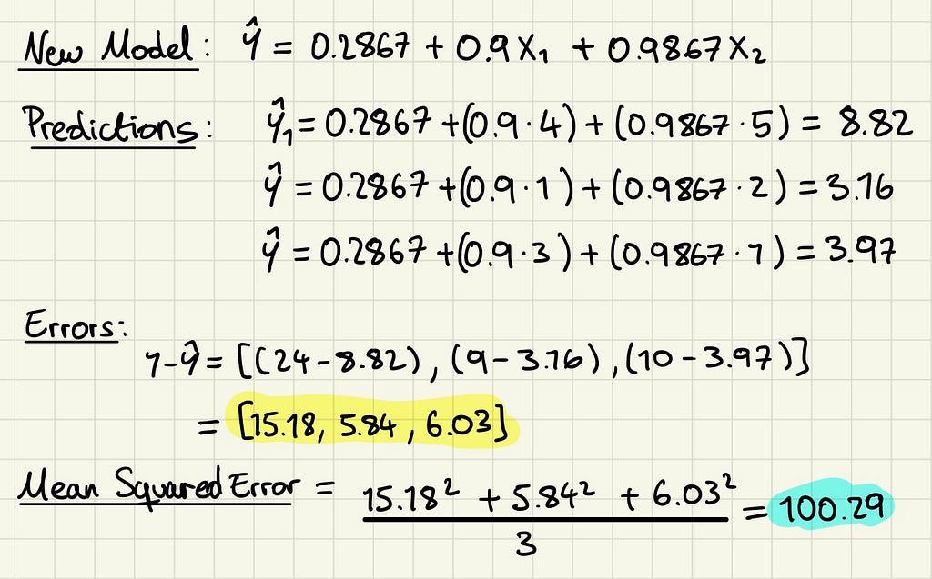
The new parameters are getting closer to the true sponge prices, and have yielded a much lower MSE, but there is a lot more training left to do. If we iterate through the gradient descent algorithm 50 times, this time using Python instead of doing it by hand — since Mr. Miyagi never said anything about coding — we will reach the following values.
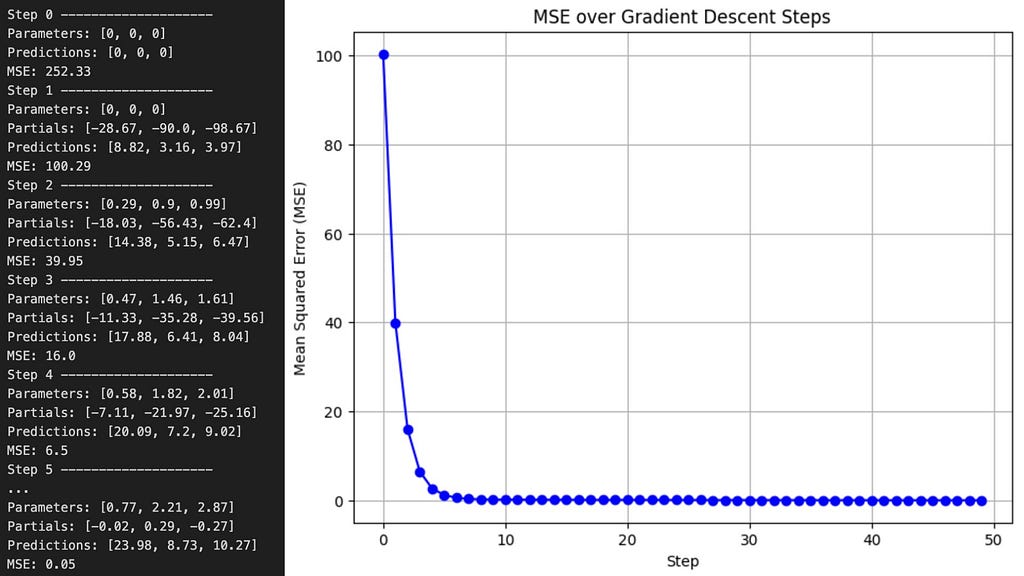
Eventually we arrived to a pretty good model. The true values I used to generate those numbers were [1, 2, 3] and after only 50 iterations, the model’s parameters came impressively close. Extending the training to 200 steps, which is another hyper-parameter, with the same learning rate allowed the linear regression model to converge almost perfectly to the true parameters, demonstrating the power of gradient descent.
Many of the fundamental concepts that make up the complicated martial art of artificial intelligence, like cost functions and gradient descent, can be thoroughly understood just by studying the simple “wax on, wax off” tool that linear regression is.
Artificial intelligence is a vast and complex field, built upon many ideas and methods. While there’s much more to explore, mastering these fundamentals is a significant first step. Hopefully, this article has brought you closer to that goal, one “wax on, wax off” at a time.
Mastering the Basics: How Linear Regression Unlocks the Secrets of Complex Models was originally published in Towards Data Science on Medium, where people are continuing the conversation by highlighting and responding to this story.
Originally appeared here:
Mastering the Basics: How Linear Regression Unlocks the Secrets of Complex Models


Accuracy is often critical for LLM applications, especially in cases such as API calling or summarisation of financial reports. Fortunately, there are ways to enhance precision. The best practices to improve accuracy include the following steps:
We’ve explored this approach in my previous TDS article, “From Prototype to Production: Enhancing LLM Accuracy”. In that project, we built an SQL Agent and went from 0% valid SQL queries to 70% accuracy. However, there are limits to what we can achieve with prompt. To break through this barrier and reach the next frontier of accuracy, we need to adopt more advanced techniques.
The most promising option is fine-tuning. With fine-tuning, we can move from relying solely on information in prompts to embedding additional information directly into the model’s weights.
Let’s start by understanding what fine-tuning is. Fine-tuning is the process of refining pre-trained models by training them on smaller, task-specific datasets to enhance their performance in particular applications. Basic models are initially trained on vast amounts of data, which allows them to develop a broad understanding of language. Fine-tuning, however, tailors these models to specialized tasks, transforming them from general-purpose systems into highly targeted tools. For example, instruction fine-tuning taught GPT-2 to chat and follow instructions, and that’s how ChatGPT emerged.
Basic LLMs are initially trained to predict the next token based on vast text corpora. Fine-tuning typically adopts a supervised approach, where the model is presented with specific questions and corresponding answers, allowing it to adjust its weights to improve accuracy.
Historically, fine-tuning required updating all model weights, a method known as full fine-tuning. This process was computationally expensive since it required storing all the model weights, states, gradients and forward activations in memory. To address these challenges, parameter-efficient fine-tuning techniques were introduced. PEFT methods update only the small set of the model parameters while keeping the rest frozen. Among these methods, one of the most widely adopted is LoRA (Low-Rank Adaptation), which significantly reduces the computational cost without compromising performance.
Before considering fine-tuning, it’s essential to weigh its advantages and limitations.
Advantages:
Disadvantages:
Since this project is focused on gaining knowledge, we will proceed with fine-tuning. However, in real-world scenarios, it’s important to evaluate whether the benefits of fine-tuning justify all the associated costs and efforts.
The next step is to plan how we will approach fine-tuning. After listening to the “Improving Accuracy of LLM Applications” course, I’ve decided to try the Lamini platform for the following reasons:
Of course, there are lots of other fine-tuning options you can consider:
As I mentioned earlier, Lamini released a new approach to fine-tuning, and I believe it’s worth discussing it in more detail.
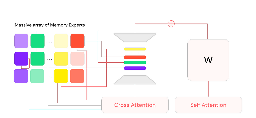
Lamini introduced the Mixture of Memory Experts (MoME) approach, which enables LLMs to learn a vast amount of factual information with almost zero loss, all while maintaining generalization capabilities and requiring a feasible amount of computational resources.
To achieve this, Lamini extended a pre-trained LLM by adding a large number (on the order of 1 million) of LoRA adapters along with a cross-attention layer. Each LoRA adapter is a memory expert, functioning as a type of memory for the model. These memory experts specialize in different aspects, ensuring that the model retains faithful and accurate information from the data it was tuned on. Inspired by information retrieval, these million memory experts are equivalent to indices from which the model intelligently retrieves and routes.
At inference time, the model retrieves a subset of the most relevant experts at each layer and merges back into the base model to generate a response to the user query.
Lamini Memory Tuning is said to be capable of achieving 95% accuracy. The key difference from traditional instruction fine-tuning is that instead of optimizing for average error across all tasks, this approach focuses on achieving zero error for the facts the model is specifically trained to remember.

So, this approach allows an LLM to preserve its ability to generalize with average error on everything else while recalling the important facts nearly perfectly.
For further details, you can refer to the research paper “Banishing LLM Hallucinations Requires Rethinking Generalization” by Li et al. (2024)
Lamini Memory Tuning holds great promise — let’s see if it delivers on its potential in practice.
As always, let’s begin by setting everything up. As we discussed, we’ll be using Lamini to fine-tune Llama, so the first step is to install the Lamini package.
pip install lamini
Additionally, we need to set up the Lamini API Key on their website and specify it as an environment variable.
export LAMINI_API_KEY="<YOUR-LAMINI-API-KEY>"
As I mentioned above, we will be improving the SQL Agent, so we need a database. For this example, we’ll continue using ClickHouse, but feel free to choose any database that suits your needs. You can find more details on the ClickHouse setup and the database schema in the previous article.
To fine-tune an LLM, we first need a dataset — in our case, a set of pairs of questions and answers (SQL queries). The task of putting together a dataset might seem daunting, but luckily, we can leverage LLMs to do it.
The key factors to consider while preparing the dataset:
All the information required to create question-and-answer pairs is present in the database schema, so it will be a feasible task for an LLM to generate examples. Additionally, I have a representative set of Q&A pairs that I used for RAG approach, which we can present to the LLM as examples of valid queries (using the few-shot prompting technique). Let’s load the RAG dataset.
# loading a set of examples
with open('rag_set.json', 'r') as f:
    rag_set = json.loads(f.read())

rag_set_df = pd.DataFrame(rag_set)

rag_set_df['qa_fmt'] = list(map(
    lambda x, y: "question: %s, sql_query: %s" % (x, y),
    rag_set_df.question,
    rag_set_df.sql_query
))
The idea is to iteratively provide the LLM with the schema information and a set of random examples (to ensure diversity in the questions) and ask it to generate a new, similar, but different Q&A pair.
Let’s create a system prompt that includes all the necessary details about the database schema.
generate_dataset_system_prompt = '''
You are a senior data analyst with more than 10 years of experience writing complex SQL queries.
There are two tables in the database you're working with with the following schemas.

Table: ecommerce.users
Description: customers of the online shop
Fields:
- user_id (integer) - unique identifier of customer, for example, 1000004 or 3000004
- country (string) - country of residence, for example, "Netherlands" or "United Kingdom"
- is_active (integer) - 1 if customer is still active and 0 otherwise
- age (integer) - customer age in full years, for example, 31 or 72

Table: ecommerce.sessions
Description: sessions for online shop
Fields:
- user_id (integer) - unique identifier of customer, for example, 1000004 or 3000004
- session_id (integer) - unique identifier of session, for example, 106 or 1023
- action_date (date) - session start date, for example, "2021-01-03" or "2024-12-02"
- session_duration (integer) - duration of session in seconds, for example, 125 or 49
- os (string) - operation system that customer used, for example, "Windows" or "Android"
- browser (string) - browser that customer used, for example, "Chrome" or "Safari"
- is_fraud (integer) - 1 if session is marked as fraud and 0 otherwise
- revenue (float) - income in USD (the sum of purchased items), for example, 0.0 or 1506.7


Write a query in ClickHouse SQL to answer the following question.
Add "format TabSeparatedWithNames" at the end of the query to get data from ClickHouse database in the right format.
'''
The next step is to create a template for the user query.
generate_dataset_qa_tmpl = '''
Considering the following examples, please, write question
and SQL query to answer it, that is similar but different to provided below.

Examples of questions and SQL queries to answer them:
{examples}
'''
Since we need a high-quality dataset, I prefer using a more advanced model — GPT-4o— rather than Llama. As usual, I’ll initialize the model and create a dummy tool for structured output.
from langchain_core.tools import tool

@tool
def generate_question_and_answer(comments: str, question: str, sql_query: str) -> str:
  """Returns the new question and SQL query

  Args:
      comments (str): 1-2 sentences about the new question and answer pair,
      question (str): new question
      sql_query (str): SQL query in ClickHouse syntax to answer the question
  """
  pass

from langchain_openai import ChatOpenAI
generate_qa_llm = ChatOpenAI(model="gpt-4o", temperature = 0.5)
  .bind_tools([generate_question_and_answer])
Now, let’s combine everything into a function that will generate a Q&A pair and create a set of examples.
# helper function to combine system + user prompts
def get_openai_prompt(question, system):
    messages = [
        ("system", system),
        ("human", question)
    ]
    return messages

def generate_qa():
  # selecting 3 random examples
  sample_set_df = rag_set_df.sample(3)
  examples = 'nn'.join(sample_set_df.qa_fmt.values)

  # constructing prompt
  prompt = get_openai_prompt(
    generate_dataset_qa_tmpl.format(examples = examples),
    generate_dataset_system_prompt)

  # calling LLM
  qa_res = generate_qa_llm.invoke(prompt)

  try:
      rec = qa_res.tool_calls[0]['args']
      rec['examples'] = examples
      return rec
  except:
      pass

# executing function
qa_tmp = []
for i in tqdm.tqdm(range(2000)):
  qa_tmp.append(generate_qa())

new_qa_df = pd.DataFrame(qa_tmp)
I generated 2,000 examples, but in reality, I used a much smaller dataset for this toy project. Therefore, I recommend limiting the number of examples to 200–300.
As we know, “garbage in, garbage out”, so an essential step before fine-tuning is cleaning the data generated by the LLM.
The first — and most obvious — check is to ensure that each SQL query is valid.
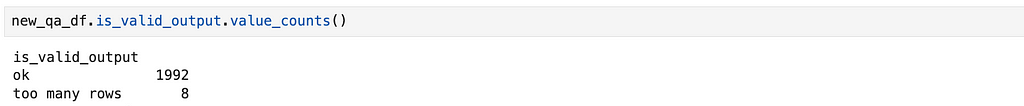
def is_valid_output(s):
    if s.startswith('Database returned the following error:'):
        return 'error'
    if len(s.strip().split('n')) >= 1000:
        return 'too many rows'
    return 'ok'

new_qa_df['output'] = new_qa_df.sql_query.map(get_clickhouse_data)
new_qa_df['is_valid_output'] = new_qa_df.output.map(is_valid_output)
There are no invalid SQL queries, but some questions return over 1,000 rows.
Although these cases are valid, we’re focusing on an OLAP scenario with aggregated stats, so I’ve retained only queries that return 100 or fewer rows.
new_qa_df['output_rows'] = new_qa_df.output.map(
  lambda x: len(x.strip().split('n')))

filt_new_qa_df = new_qa_df[new_qa_df.output_rows <= 100]
I also eliminated cases with empty output — queries that return no rows or only the header.
filt_new_qa_df = filt_new_qa_df[filt_new_qa_df.output_rows > 1]
Another important check is for duplicate questions. The same question with different answers could confuse the model, as it won’t be able to tune to both solutions simultaneously. And in fact, we have such cases.
filt_new_qa_df = filt_new_qa_df[['question', 'sql_query']].drop_duplicates()
filt_new_qa_df['question'].value_counts().head(10)
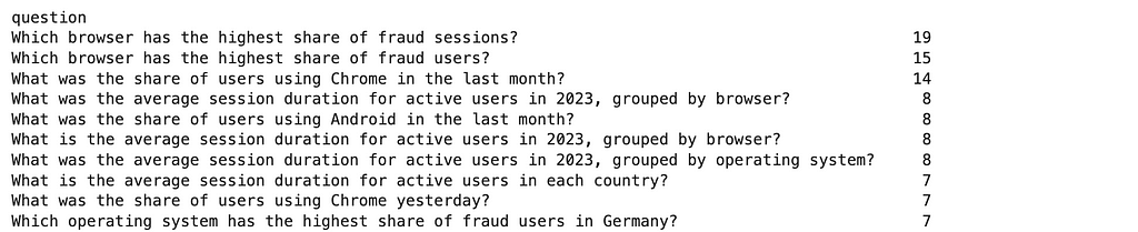
To resolve these duplicates, I’ve kept only one answer for each question.
filt_new_qa_df = filt_new_qa_df.drop_duplicates('question')
Although I generated around 2,000 examples, I’ve decided to use a smaller dataset of 200 question-and-answer pairs. Fine-tuning with a larger dataset would require more tuning steps and be more expensive.
sample_dataset_df = pd.read_csv('small_sample_for_finetuning.csv', sep = 't')
You can find the final training dataset on GitHub.
Now that our training dataset is ready, we can move on to the most exciting part — fine-tuning.
The next step is to generate the sets of requests and responses for the LLM that we will use to fine-tune the model.
Since we’ll be working with the Llama model, let’s create a helper function to construct a prompt for it.
def get_llama_prompt(user_message, system_message=""):
    system_prompt = ""
    if system_message != "":
        system_prompt = (
            f"<|start_header_id|>system<|end_header_id|>nn{system_message}"
            f"<|eot_id|>"
        )
    prompt = (f"<|begin_of_text|>{system_prompt}"
              f"<|start_header_id|>user<|end_header_id|>nn"
              f"{user_message}"
              f"<|eot_id|>"
              f"<|start_header_id|>assistant<|end_header_id|>nn"
         )
    return prompt
For requests, we will use the following system prompt, which includes all the necessary information about the data schema.
generate_query_system_prompt = '''
You are a senior data analyst with more than 10 years of experience writing complex SQL queries.
There are two tables in the database you're working with with the following schemas.

Table: ecommerce.users
Description: customers of the online shop
Fields:
- user_id (integer) - unique identifier of customer, for example, 1000004 or 3000004
- country (string) - country of residence, for example, "Netherlands" or "United Kingdom"
- is_active (integer) - 1 if customer is still active and 0 otherwise
- age (integer) - customer age in full years, for example, 31 or 72

Table: ecommerce.sessions
Description: sessions of usage the online shop
Fields:
- user_id (integer) - unique identifier of customer, for example, 1000004 or 3000004
- session_id (integer) - unique identifier of session, for example, 106 or 1023
- action_date (date) - session start date, for example, "2021-01-03" or "2024-12-02"
- session_duration (integer) - duration of session in seconds, for example, 125 or 49
- os (string) - operation system that customer used, for example, "Windows" or "Android"
- browser (string) - browser that customer used, for example, "Chrome" or "Safari"
- is_fraud (integer) - 1 if session is marked as fraud and 0 otherwise
- revenue (float) - income in USD (the sum of purchased items), for example, 0.0 or 1506.7


Write a query in ClickHouse SQL to answer the following question.
Add "format TabSeparatedWithNames" at the end of the query to get data from ClickHouse database in the right format.
Answer questions following the instructions and providing all the needed information and sharing your reasoning.
'''
Let’s create the responses in the format suitable for Lamini fine-tuning. We need to prepare a list of dictionaries with input and output keys.
formatted_responses = []

for rec in sample_dataset_df.to_dict('records'):
  formatted_responses.append(
    {
      'input': get_llama_prompt(rec['question'],
        generate_query_system_prompt),
      'output': rec['sql_query']
    }
  )
Now, we are fully prepared for fine-tuning. We just need to select a model and initiate the process. We will be fine-tuning the Llama 3.1 8B model.
from lamini import Lamini
llm = Lamini(model_name="meta-llama/Meta-Llama-3.1-8B-Instruct")

finetune_args = {
    "max_steps": 50,
    "learning_rate": 0.0001
}

llm.train(
  data_or_dataset_id=formatted_responses,
  finetune_args=finetune_args,
)
We can specify several hyperparameters, and you can find all the details in the Lamini documentation. For now, I’ve passed only the most essential ones to the function:
Now, we just need to wait for 10–15 minutes while the model trains, and then we can test it.
finetuned_llm = Lamini(model_name='<model_id>')
# you can find Model ID in the Lamini interface

question = '''How many customers made purchase in December 2024?'''
prompt = get_llama_prompt(question, generate_query_system_prompt)
finetuned_llm.generate(prompt, max_new_tokens=200)
# select uniqExact(s.user_id) as customers
# from ecommerce.sessions s join ecommerce.users u
# on s.user_id = u.user_id
# where (toStartOfMonth(action_date) = '2024-12-01') and (revenue > 0)
# format TabSeparatedWithNames
It’s worth noting that we’re using Lamini for inference as well and will have to pay for it. You can find up-to-date information about the costs here.
At first glance, the result looks promising, but we need a more robust accuracy evaluation to confirm it.
Additionally, it’s worth noting that since we’ve fine-tuned the model for our specific task, it now consistently returns SQL queries, meaning we may no longer need to use tool calls for structured output.
We’ve discussed LLM accuracy evaluation in detail in my previous article, so here I’ll provide a brief recap.
We use a golden set of question-and-answer pairs to evaluate the model’s quality. Since this is a toy example, I’ve limited the set to just 10 pairs, which you can review on GitHub.
The evaluation process consists of two parts:
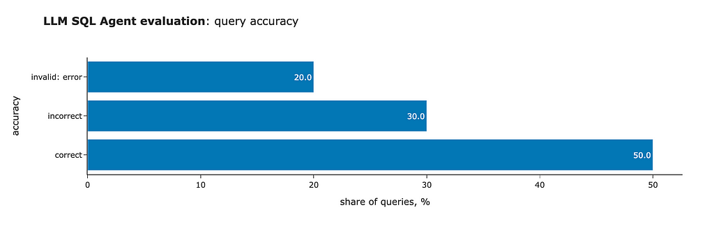
The initial results are far from ideal, but they are significantly better than the base Llama model (which produced zero valid SQL queries). Here’s what we found:
No surprises — there’s no silver bullet, and it’s always an iterative process. Let’s investigate what went wrong.
The approach is straightforward. Let’s examine the errors one by one to understand why we got these results and how we can fix them. We’ll start with the first unsuccessful example.
Question: Which country had the highest number of first-time users in 2024?
Golden query:
select
  country,
  count(distinct user_id) as users
from
  (
    select user_id, min(action_date) as first_date
    from ecommerce.sessions
    group by user_id
    having toStartOfYear(first_date) = '2024-01-01'
  ) as t
  inner join ecommerce.users as u
    on t.user_id = u.user_id
group by country
order by users desc
limit 1
format TabSeparatedWithNames
Generated query:
select
  country,
  count(distinct u.user_id) as first_time_users
from ecommerce.sessions s
join ecommerce.users u
  on s.user_id = u.user_id
where (toStartOfYear(action_date) = '2024-01-01')
  and (s.session_id = 1)
group by country
order by first_time_users desc
limit 1
format TabSeparatedWithNames
The query is valid, but it returns an incorrect result. The issue lies in the model’s assumption that the first session for each user will always have session_id = 1. Since Lamini Memory Tuning allows the model to learn facts from the training data, let’s investigate why the model made this assumption. Likely, it’s in our data.
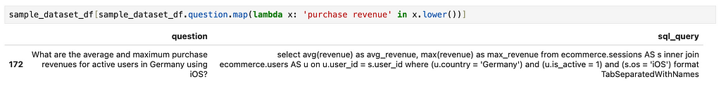
Let’s review all the examples that mention first. I’ll use broad and simple search criteria to get a high-level view.
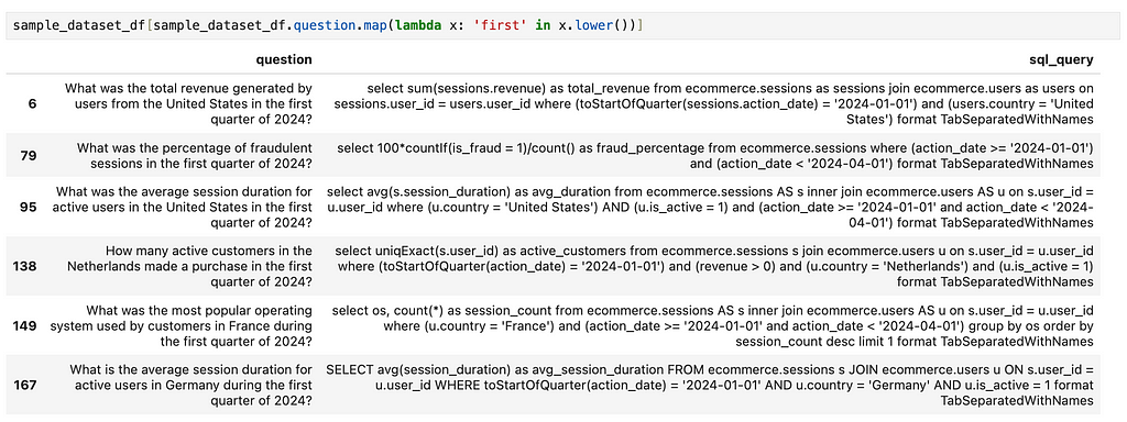
As we can see, there are no examples mentioning first-time users — only references to the first quarter. It’s no surprise that the model wasn’t able to capture this concept. The solution is straightforward: we just need to add a set of examples with questions and answers specifically about first-time users.
Let’s move on to the next problematic case.
Question: What was the fraud rate in 2023, expressed as a percentage?
Golden query:
select
  100*uniqExactIf(user_id, is_fraud = 1)/uniqExact(user_id) as fraud_rate
from ecommerce.sessions
where (toStartOfYear(action_date) = '2023-01-01')
format TabSeparatedWithNames
Generated query:
select
  100*countIf(is_fraud = 1)/count() as fraud_rate
from ecommerce.sessions
where (toStartOfYear(action_date) = '2023-01-01')
format TabSeparatedWithNames
Here’s another misconception: we assumed that the fraud rate is based on the share of users, while the model calculated it based on the share of sessions.
Let’s check the examples related to the fraud rate in the data. There are two cases: one calculates the share of users, while the other calculates the share of sessions.
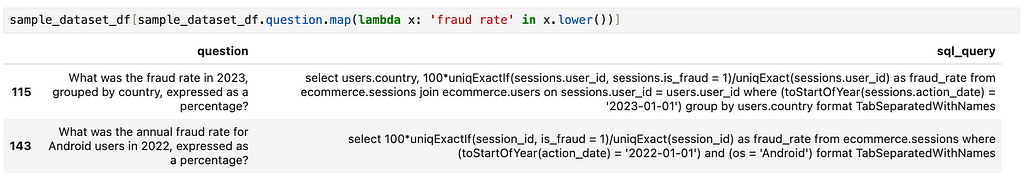
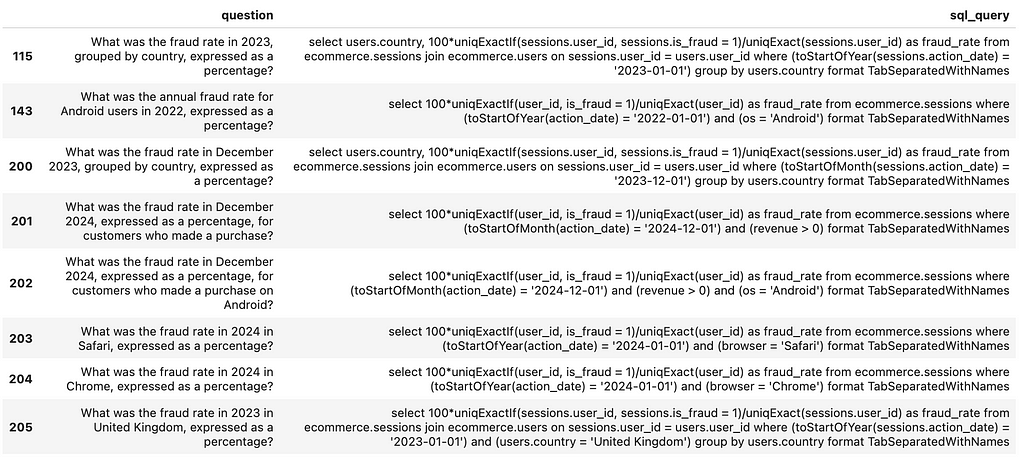
To fix this issue, I corrected the incorrect answer and added more accurate examples involving fraud rate calculations.
I’d like to discuss another incorrect case, as it will highlight an important aspect of the process of resolving these issues.
Question: What are the median and interquartile range (IQR) of purchase revenue for each country?
Golden query:
select
  country,
  median(revenue) as median_revenue,
  quantile(0.25)(revenue) as percentile_25_revenue,
  quantile(0.75)(revenue) as percentile_75_revenue
from ecommerce.sessions AS s
inner join ecommerce.users AS u
  on u.user_id = s.user_id
where (revenue > 0)
group by country
format TabSeparatedWithNames
Generated query:
select
  country,
  median(revenue) as median_revenue,
  quantile(0.25)(revenue) as percentile_25_revenue,
  quantile(0.75)(revenue) as percentile_75_revenue
from ecommerce.sessions s join ecommerce.users u
  on s.user_id = u.user_id
group by country
format TabSeparatedWithNames
When inspecting the problem, it’s crucial to focus on the model’s misconceptions or incorrect assumptions. For example, in this case, there may be a temptation to add examples similar to those in the golden dataset, but that would be too specific. Instead, we should address the actual root cause of the model’s misconception:
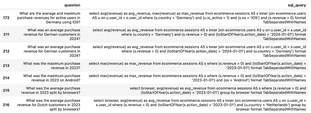
So, we need to ensure that our datasets contain enough information related to purchase revenue. Let’s take a look at what we have now. There’s only one example, and it’s incorrect.
Let’s fix this example and add more cases of purchase revenue calculations.
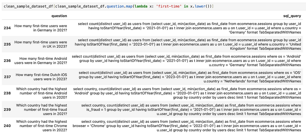
Using a similar approach, I’ve added more examples for the two remaining incorrect queries and compiled an updated, cleaned version of the training dataset. You can find it on GitHub. With this, our data is ready to the next iteration.
Before diving into fine-tuning, it’s essential to double-check the quality of the training dataset by ensuring that all SQL queries are valid.
clean_sample_dataset_df = pd.read_csv(
  'small_sample_for_finetuning_cleaned.csv', sep = 't',
  on_bad_lines = 'warn')

clean_sample_dataset_df['output'] = clean_sample_dataset_df.sql_query
  .map(lambda x: get_clickhouse_data(str(x)))
clean_sample_dataset_df['is_valid_output'] = clean_sample_dataset_df['output']
  .map(is_valid_output)
print(clean_sample_dataset_df.is_valid_output.value_counts())

# is_valid_output
# ok    241

clean_formatted_responses = []
for rec in clean_sample_dataset_df.to_dict('records'):
  clean_formatted_responses.append(
    {
      'input': get_llama_prompt(
        rec['question'],
        generate_query_system_prompt),
      'output': rec['sql_query']
    }
  )
Now that we’re confident in the data, we can proceed with fine-tuning. This time, I’ve decided to train it for 150 steps to achieve better accuracy.
finetune_args = {
      "max_steps": 150,
      "learning_rate": 0.0001
}

llm = Lamini(model_name="meta-llama/Meta-Llama-3.1-8B-Instruct")
llm.train(
  data_or_dataset_id=clean_formatted_responses,
  finetune_args=finetune_args
)
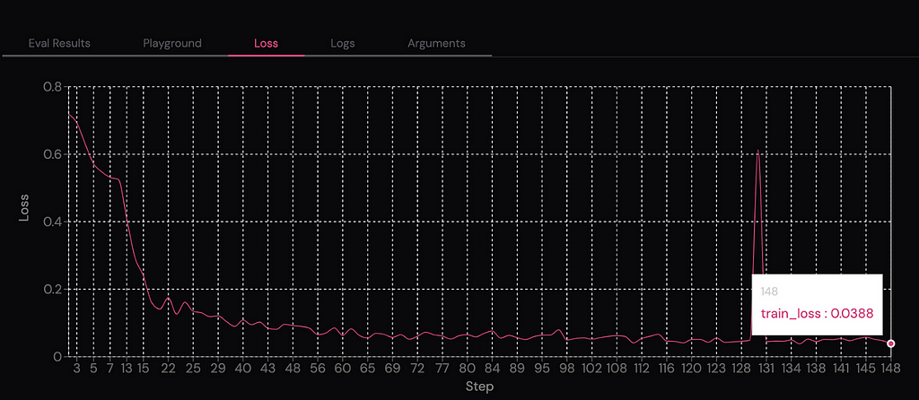
After waiting a bit longer than last time, we now have a new fine-tuned model with nearly zero loss after 150 tuning steps.
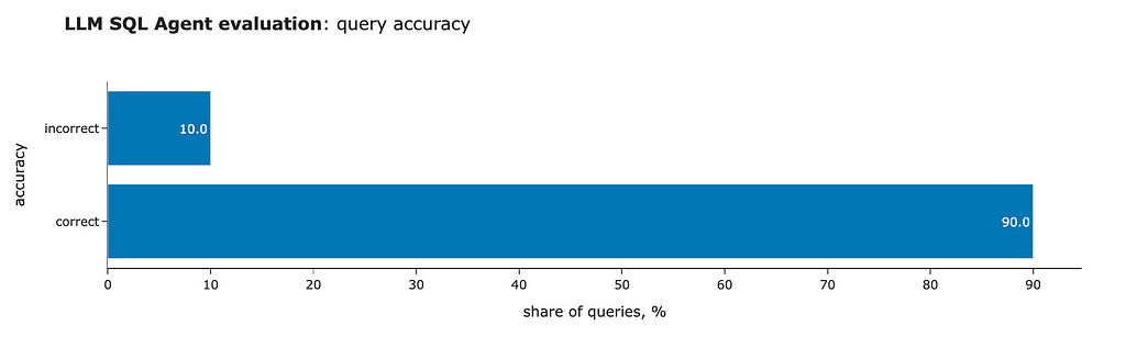
We can run the evaluation again and see much better results. So, our approach is working.
The result is astonishing, but it’s still worth examining the incorrect example to understand what went wrong. We got an incorrect result for the question we discussed earlier: “What are the median and interquartile range (IQR) of purchase revenue for each country?” However, this time, the model generated a query that is exactly identical to the one in the golden set.
select
  country,
  median(revenue) as median_revenue,
  quantile(0.25)(revenue) as percentile_25_revenue,
  quantile(0.75)(revenue) as percentile_75_revenue
from ecommerce.sessions AS s
inner join ecommerce.users AS u
  on u.user_id = s.user_id
where (s.revenue > 0)
group by country
format TabSeparatedWithNames
So, the issue actually lies in our evaluation. In fact, if you try to execute this query multiple times, you’ll notice that the results are slightly different each time. The root cause is that the quantile function in ClickHouse computes approximate values using reservoir sampling, which is why we’re seeing varying results. We could have used quantileExact instead to get more consistent numbers.
That said, this means that fine-tuning has allowed us to achieve 100% accuracy. Even though our toy golden dataset consists of just 10 questions, this is a tremendous achievement. We’ve progressed all the way from zero valid queries with vanilla Llama to 70% accuracy with RAG and self-reflection, and now, thanks to Lamini Memory Tuning, we’ve reached 100% accuracy.
You can find the full code on GitHub.
In this article, we continued exploring techniques to improve LLM accuracy:
Thank you a lot for reading this article. I hope this article was insightful for you. If you have any follow-up questions or comments, please leave them in the comments section.
All the images are produced by the author unless otherwise stated.
This article is inspired by the “Improving Accuracy of LLM Applications” short course from DeepLearning.AI.
Disclaimer: I am not affiliated with Lamini in any way. The views expressed in this article are solely my own, based on independent testing and evaluation of the Lamini platform. This post is intended for educational purposes and does not constitute an endorsement of any specific tool or service.
The Next Frontier in LLM Accuracy was originally published in Towards Data Science on Medium, where people are continuing the conversation by highlighting and responding to this story.
Originally appeared here:
The Next Frontier in LLM Accuracy
Go Here to Read this Fast! The Next Frontier in LLM Accuracy