AWS offers powerful generative AI services, including Amazon Bedrock, which allows organizations to create tailored use cases such as AI chat-based assistants that give answers based on knowledge contained in the customers’ documents, and much more. Many businesses want to integrate these cutting-edge AI capabilities with their existing collaboration tools, such as Google Chat, to […]
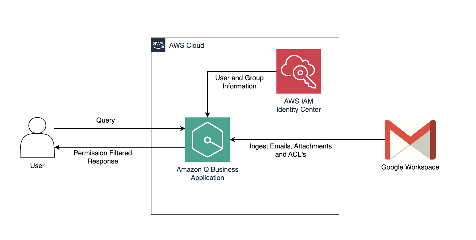
A number of organizations use Gmail for their business email needs. Gmail for business is part of Google Workspace, which provides a set of productivity and collaboration tools like Google Drive, Gmail, and Google Calendar. Google Drive supports storing documents such as Emails contain a wealth of information found in different places, such as within […]
Amazon SageMaker Ground Truth enables the creation of high-quality, large-scale training datasets, essential for fine-tuning across a wide range of applications, including large language models (LLMs) and generative AI. By integrating human annotators with machine learning, SageMaker Ground Truth significantly reduces the cost and time required for data labeling. Whether it’s annotating images, videos, or […]
We seem to be in that sweet spot on the calendar between the end of summer and the final rush before things slow down for the holiday season—in other words, it’s the perfect time of year for learning, tinkering, and exploration.
Our most-read articles from October reflect this spirit of focused energy, covering a slew of hands-on topics. From actionable AI project ideas and data science revenue streams to accessible guides on time-series analysis and LLMs, these stories do a great job representing the breadth of our authors’ expertise and the diversity of their (and our readers’) interests. If you haven’t read them yet, what better time than now?
Monthly Highlights
5 AI Projects You Can Build This Weekend (with Python) If your sleeves aren’t rolled up just yet, they will be shortly: our most-read post in October, from Shaw Talebi, outlines several compelling project ideas for anyone who’s been thinking about putting their AI knowledge into action. From resume organizers to a multimodal search tool, they offer a smooth entryway into the ever-expanding world of AI-powered product development.
LLM Evaluation Skills Are Easy to Pick Up (Yet Costly to Practice) Creating LLM solutions requires a major investment of time and resources, which makes it crucial for product managers and ML engineers to get a clear and accurate sense of their performance. Thuwarakesh Murallie walks us through the nitty-gritty details of leveraging several evaluation approaches and tools to achieve that often-elusive goal.
Top 5 Principles for Building User-Friendly Data Tables “There are numerous times I wonder, ‘What does this column mean?’ ‘Why are there two columns with the same name in table A and table B? Which one should I use?’” Yu Dong introduces five useful rules that will ensure your data tables are accessible, usable, and easily interpretable for teammates and other stakeholders.
How I Studied LLMs in Two Weeks: A Comprehensive Roadmap While you might think that LLMs have been inescapable for the past couple of years, many practitioners — both new and seasoned — are just beginning to tune in to this buzzing topic; for a structured approach to learning all the basics (and then some), head right over to Hesam Sheikh’s well-received curriculum.
Understanding LLMs from Scratch Using Middle School Math If you could use a more guided method to learn about large language models from the ground up, give Rohit Patel’s debut TDS contribution a try: it’s a comprehensive, 40-minute explainer on these models’ inner workings—and requires no advanced math or machine learning knowledge.
AI Agents: The Intersection of Tool Calling and Reasoning in Generative AI Few topics in recent months have generated as much buzz as AI agents; if you’d like to deepen your understanding of their potential (and limitations), don’t miss Tula Masterman’s lucid overview, which focuses on how agent reasoning is expressed through tool calling, explores some of the challenges agents face with tool use, and covers common ways to evaluate their tool-calling ability.
My 7 Sources of Income as a Data Scientist Most (all?) data professionals know about the perks of working full time at a tech giant, but the options for monetizing your skills are much broader than that. Egor Howell provides a candid breakdown of the various revenue streams he’s cultivated in the past few years since becoming a full-time data scientist.
Thank you for supporting the work of our authors! We love publishing articles from new authors, so if you’ve recently written an interesting project walkthrough, tutorial, or theoretical reflection on any of our core topics, don’t hesitate to share it with us.
We hear a lot about productionized machine learning, but what does it really mean to have a model that can thrive in real-world applications?There are plenty of things that go into, and contribute, to the efficacy of a machine learning model in production. For the sake of this article we will be focusing on five of them.
Reproducibility
Monitoring
Testing
Automation
Version Control
Serving Inferences
The most important part of building a production-ready machine learning model is being able to access it.
For this purpose, we build a fastapi client that serves sentiment analysis responses. We utilize pydantic to ensure structure for the input and output. The model that we use is the base sentiment analysis pipeline from huggingface’s transformers library, allowing us to begin testing with a pre-trained model.
# Filename: main.py from fastapi import FastAPI from pydantic import BaseModel from transformers import pipeline
To install this, initialize venv in your files and run:pip install -r requirements.txt.
To host this API simply run: uvicorn main:app –reload.
Now you have an api that you can query using:
curl -X POST "http://localhost:8000/predict"
  -H "Content-Type: application/json"
  -d '{"text": "I love using FastAPI!"}'
or any API tool you wish (i.e. Postman). You should get a result back that includes the text query, the sentiment predicted, and the confidence of the prediction.
We now have a locally hosted machine learning inference API.
Further Improving Reproducibility
To allow our code to have more consistent execution, we will utilize Docker. Docker simulates a lightweight environment that allows applications to run in isolated containers, similar to virtual machines. This isolation ensures that applications can execute consistently across any computer with Docker installed, regardless of the underlying system.
Now, you can build the image and run this API using:
# Build the Docker image
docker build -t sentiment-api .

# Run the container
docker run -p 8000:8000 sentiment-api
You should now be able to query just as you did before.
curl -X POST "http://localhost:8000/predict"
  -H "Content-Type: application/json"
  -d '{"text": "I love using FastAPI!"}'
We now have a containerized, locally hosted machine learning inference API.
Adding Basic Monitoring
In machine learning applications, monitoring is crucial for understanding model performance and ensuring it meets expected accuracy and efficiency. Tools like Prometheus help track metrics such as prediction latency, request counts, and model output distributions, enabling you to identify issues like model drift or resource bottlenecks. This proactive approach ensures that your ML models remain effective over time and can adapt to changing data or usage patterns. In our case, we are focused on prediction time, requests, and gathering information about our queries.
from fastapi import FastAPI from pydantic import BaseModel from transformers import pipeline from prometheus_client import Counter, Histogram, start_http_server import time
# Start prometheus metrics server on port 8001 start_http_server(8001)
While the process of building and fine-tuning a model is not the intent of this project, it is important to understand how a model can be added to this process.
# Filename: train.py
import torch from transformers import AutoTokenizer, AutoModelForSequenceClassification from datasets import load_dataset from torch.utils.data import DataLoader
# Use GPU if available device = torch.device("cuda" if torch.cuda.is_available() else "cpu") model.to(device)
model.train()
# Create a DataLoader for batching dataloader = DataLoader(dataset, batch_size=8, shuffle=True)
# Training loop num_epochs = 3 # Set the number of epochs for epoch in range(num_epochs): total_loss = 0 for batch in dataloader: inputs = tokenizer(batch["text"], truncation=True, padding=True, return_tensors="pt", max_length=512).to(device) labels = torch.tensor(batch["label"]).to(device)
optimizer.zero_grad() outputs = model(**inputs, labels=labels) loss = outputs.loss
# Save the model model.save_pretrained("./model/") tokenizer.save_pretrained("./model/")
# Test the model with sample sentences test_sentences = [ "This movie was fantastic!", "I absolutely hated this film.", "It was just okay, not great.", "An absolute masterpiece!", "Waste of time!", "A beautiful story and well acted.", "Not my type of movie.", "It could have been better.", "A thrilling adventure from start to finish!", "Very disappointing." ]
# Switch model to evaluation mode model.eval()
# Prepare tokenizer for test inputs inputs = tokenizer(test_sentences, truncation=True, padding=True, return_tensors="pt", max_length=512).to(device)
with torch.no_grad(): outputs = model(**inputs) predictions = torch.argmax(outputs.logits, dim=1)
# Print predictions for sentence, prediction in zip(test_sentences, predictions): sentiment = "positive" if prediction.item() == 1 else "negative" print(f"Input: "{sentence}" -> Predicted sentiment: {sentiment}")
# Call the function to train the model and test it train_model()
To make sure that we can query our new model that we have trained we have to update a few of our existing files. For instance, in main.py we now use the model from ./model and load it as a pretrained model. Additionally, for comparison’s sake, we add now have two endpoints to use, /predict/naive and predict/trained.
# Filename: main.py
from fastapi import FastAPI from pydantic import BaseModel from transformers import AutoModelForSequenceClassification, AutoTokenizer from transformers import pipeline from prometheus_client import Counter, Histogram, start_http_server import time
# Start prometheus metrics server on port 8001 start_http_server(8001)
app = FastAPI()
# Load the trained model and tokenizer from the local directory model_path = "./model" # Path to your saved model tokenizer = AutoTokenizer.from_pretrained(model_path) trained_model = AutoModelForSequenceClassification.from_pretrained(model_path)
Importantly, if you are using git, make sure that you add the pytorch_model.bin file to git lfs, so that you can push to GitHub. git lfs allows you to use version control on very large files.
Adding Testing and CI/CD
CI/CD and testing streamline the deployment of machine learning models by ensuring that code changes are automatically integrated, tested, and deployed, which reduces the risk of errors and enhances model reliability. This process promotes continuous improvement and faster iteration cycles, allowing teams to deliver high-quality, production-ready models more efficiently. Firstly, we create two very basic tests to ensure that our model is performing acceptably.
# Filename: test_model.py
import pytest from fastapi.testclient import TestClient from main import app
Now, whenever we push to GitHub, it will run an automated process that checks out the code, sets up a Python 3.9 environment, installs dependencies, and runs our tests using pytest.
Conclusion
In this project, we’ve developed a production-ready sentiment analysis API that highlights key aspects of deploying machine learning models. While it doesn’t encompass every facet of the field, it provides a representative sampling of essential tasks involved in the process. By examining these components, I hope to clarify concepts you may have encountered but weren’t quite sure how they fit together in a practical setting.
Minimum Viable MLE was originally published in Towards Data Science on Medium, where people are continuing the conversation by highlighting and responding to this story.
Storage accounts play a vital role in a medallion architecture for establishing an enterprise data lake. They act as a centralized repository, enabling seamless data exchange between producers and consumers. This setup empowers consumers to perform data science tasks and build machine learning (ML) models. Furthermore, consumers can use the data for Retrieval Augmented Generation (RAG), facilitating interaction with company data through Large Language Models (LLMs) like ChatGPT.
Highly sensitive data is typically stored in the storage account. Defense in depth measures must be in place before data scientists and ML pipelines can access the data. To do defense in depth, multiple measurement shall be in place such as 1) advanced threat protection to detect malware, 2) authentication using Microsoft Entra, 3) authorization to do fine grained access control, 4) audit trail to monitor access, 5) data exfiltration prevention, 6) encryption, and last but not least 7) network access control using service endpoint or private endpoints.
This article focuses on network access control of the storage account. In the next chapter, the different concepts are explained (demystified) on storage account network access. Following that, a hands-on comparison is done between service endpoint and private endpoints. Finally, a conclusion is drawn.
2. Discuss network access possibilities
A typical scenario is that a virtual machine needs to have network access to a storage account. This virtual machine often acts as a Spark cluster to analyze data from the storage account. The image below provides an overview of the available network access controls.
2.1 Overview of networking between virtual machine and storage account — image by author
The components in the image can be described as follows:
Azure global network — backbone: Traffic always goes over Azure backbone between two regions (unless customer forces to not do it), see also Microsoft global network — Azure | Microsoft Learn. This is regardless of what firewall rule is used in the storage account and regardless whether service endpoints or private endpoints are used.
Azure storage firewalls: Firewall rules can restrict or disable public access. Common rules include whitelisting VNET/subnet, public IP addresses, system-assigned managed identities as resource instances, or allowing trusted services. When a VNET/subnet is whitelisted, the Azure Storage account identifies the traffic’s origin and its private IP address. However, the storage account itself is not integrated into the VNET/subnet — private endpoints are needed for that purpose.
Virtual Network (VNET): Network in which virtual machines are deployed. While a storage account is never deployed within a VNET, the VNET can be whitelisted in the Azure storage firewall. Alternatively, the VNET can create a private endpoint for secure, private connectivity.
Service endpoints: When whitelisting a VNET/subnet in the Storage account firewall, the service endpoint must be turned on for the VNET/subnet. The service endpoint should beMicrosoft.Storage when the VNET and storage account are in the same region or Microsoft.Storage.Global when the VNET and storage are in different regions. Note that service endpoints is also used as an overarching term, encompassing both the whitelisting of a VNET/subnet on the Azure Storage Firewall and the enabling of the service endpoint on the VNET/subnet.
Private endpoints: Integrating a Network Interface Card (NIC) of a Storage Account within the VNET where the virtual machine operates. This integration assigns the storage account a private IP address, making it part of the VNET.
Private DNS storage account: Within a VNET, a private DNS zone can be created in which the storage account DNS resolves to the private endpoint. This is to make sure that virtual machine can still connect to the URL of the storage account and the URL of the storage account resolves to a private IP address rather than a public address.
Network Security Group (NSG): Deploy an NSG to limit inbound and outbound access of the VNET where the virtual machine runs. This can prevent data exfiltration. However, an NSG works only with IP addresses or tags, not with URLs. For more advanced data exfiltration protection, use an Azure Firewall. For simplicity, the article omits this and uses NSG to block outbound traffic.
In the next chapter, service endpoints and private endpoints are discussed.
3. Hands-on Service endpoint and private endpoints
The chapter begins by exploring the scenario of unrestricted network access. Then the details of service endpoints and private endpoints are discussed with practical examples.
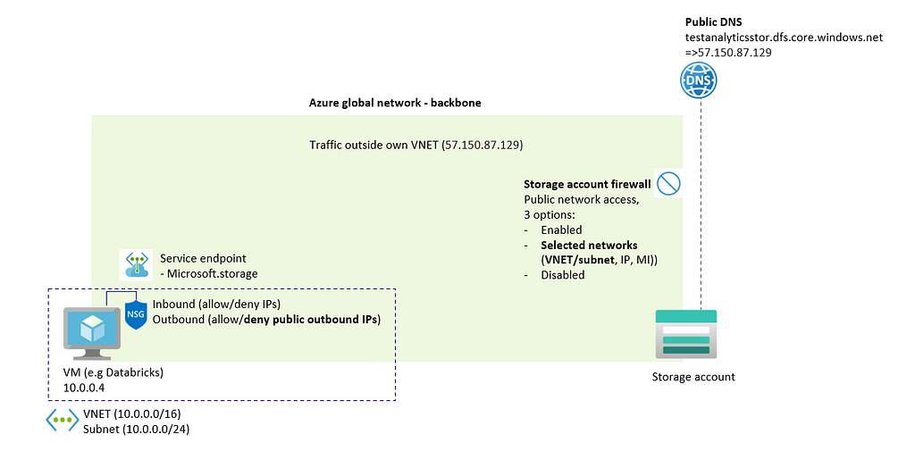
3.1 Not limiting network access — public access enabled
Suppose the following scenario in which a virtual machine and a storage account is created. The firewall of the storage account has public access enabled, see image below.
3.1.1 virtual machine and storage account with public access created
Using this configuration, a the virtual machine can access the storage account over the network. Since the virtual machine is also deployed in Azure, traffic will go over Azure Backbone and will be accepted, see image below.
3.1.2 Traffic not blocked — public network access enabled
Enterprises typically establish firewall rules to limit network access. This involves disabling public access or allowing only selected networks and whitelisting specific ones. The image below illustrates public access being disabled and traffic being blocked by the firewall.
3.1.3 Traffic blocked — blocking traffic in storage account firewall
In the next paragraph, service endpoints and selected network firewall rules are used to grant network access to storage account again.
3.2 Limiting network access via Service endpoints
To enable virtual machine VNET access to the storage account, activate the service endpoint on the VNET. Use Microsoft.Storage for within the regions or Microsoft.Storage.Global for cross region. Next, whitelist the VNET/subnet in the storage account firewall. Traffic is then blocked again, see also image below.
3.2.1 Traffic not blocked — service endpoint enabled and added to in storage account firewall
Traffic is now accepted. When VNET/subnet is removed from Azure storage account firewall or public access is disabled, then traffic is blocked again.
In case an NSG is used to block public outbound IPs in the VNET of the virtual machine, then traffic is also blocked again. This is because the public DNS of the storage account is used, see also image below.
3.2.2 Traffic blocked — NSG of virtual machine blocking public outbound traffic
In that case, private endpoints shall be used to make sure that traffic does not leave VNET. This is discussed in the next chapter.
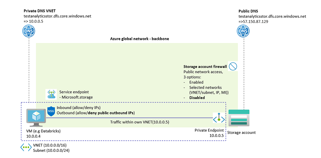
3.3 Limiting access via Private endpoints
To reestablish network access for the virtual machine to the storage account, use a private endpoint. This action creates a network interface card (NIC) for the storage account within the VNET of the virtual machine, ensuring that traffic remains within the VNET. The image below provides further illustration.
3.3.1 Traffic not blocked — Private endpoint created to Storage account, public access disabled
Again, an NSG can be used again to block all traffic, see image below.
3.3.2 Traffic blocked — NSG of virtual machine blocking all outbound traffic
This is however counterintuitive, since first a private endpoint is created in the VNET and then traffic is blocked by NSG in the same VNET.
3. Conclusion
Enterprise always requires network rules in place to limit network access to their storage account. In this blog post, both service endpoints and private endpoint are considered to limit access.
Both is true for service endpoints and private endpoints:
Traffic always goes over Azure backbone between two regions (unless customer forces to not do it), see also Microsoft global network — Azure | Microsoft Learn. This is regardless of what firewall rule is used in the storage account. Also, it is independent whether service endpoints or private endpoints are used.
Requires to enable service endpoints on VNET/subnet and whitelisting of VNET/subnet in Azure storage account firewall.
Requires that traffic leaves the VNET of the virtual machine that is connecting to the storage account. See above, the traffic stays on the Azure backbone.
For private endpoints, the following hold:
Public access can be disabled in the Azure Storage firewall. See above, public DNS entry of storage account will remain.
Traffic does not leave the VNET in which the virtual machine also runs.
There are a lot of other things to consider whether to use service endpoints or private endpoints (costs, migration effort since service endpoints have been out there longer than private endpoints, networking complexity when using private endpoints, limited service endpoint support of newer Azure services, hard limit of number private endpoints in storage account of 200).
However, in case it is required (“must have”) that 1) traffic shall never leave VNET/subnet of virtual machine or 2) it is not allowed to create firewall rules in Azure storage firewall and must be locked down, then service endpoint is not feasible.
In other scenarios, it’s possible to consider both solutions, and the best fit should be determined based on the specific requirements of each scenario.
We use cookies on our website to give you the most relevant experience by remembering your preferences and repeat visits. By clicking “Accept”, you consent to the use of ALL the cookies.
This website uses cookies to improve your experience while you navigate through the website. Out of these, the cookies that are categorized as necessary are stored on your browser as they are essential for the working of basic functionalities of the website. We also use third-party cookies that help us analyze and understand how you use this website. These cookies will be stored in your browser only with your consent. You also have the option to opt-out of these cookies. But opting out of some of these cookies may affect your browsing experience.
Necessary cookies are absolutely essential for the website to function properly. These cookies ensure basic functionalities and security features of the website, anonymously.
Cookie
Duration
Description
cookielawinfo-checkbox-analytics
11 months
This cookie is set by GDPR Cookie Consent plugin. The cookie is used to store the user consent for the cookies in the category "Analytics".
cookielawinfo-checkbox-functional
11 months
The cookie is set by GDPR cookie consent to record the user consent for the cookies in the category "Functional".
cookielawinfo-checkbox-necessary
11 months
This cookie is set by GDPR Cookie Consent plugin. The cookies is used to store the user consent for the cookies in the category "Necessary".
cookielawinfo-checkbox-others
11 months
This cookie is set by GDPR Cookie Consent plugin. The cookie is used to store the user consent for the cookies in the category "Other.
cookielawinfo-checkbox-performance
11 months
This cookie is set by GDPR Cookie Consent plugin. The cookie is used to store the user consent for the cookies in the category "Performance".
viewed_cookie_policy
11 months
The cookie is set by the GDPR Cookie Consent plugin and is used to store whether or not user has consented to the use of cookies. It does not store any personal data.
Functional cookies help to perform certain functionalities like sharing the content of the website on social media platforms, collect feedbacks, and other third-party features.
Performance cookies are used to understand and analyze the key performance indexes of the website which helps in delivering a better user experience for the visitors.
Analytical cookies are used to understand how visitors interact with the website. These cookies help provide information on metrics the number of visitors, bounce rate, traffic source, etc.
Advertisement cookies are used to provide visitors with relevant ads and marketing campaigns. These cookies track visitors across websites and collect information to provide customized ads.