Generative AI has transformed customer support, offering businesses the ability to respond faster, more accurately, and with greater personalization. AI agents, powered by large language models (LLMs), can analyze complex customer inquiries, access multiple data sources, and deliver relevant, detailed responses. In this post, we guide you through integrating Amazon Bedrock Agents with enterprise data […]
The roadmap to success in data science offers many different paths, but most of them include a strong focus on math and programming skills (case in point: this excellent guide for aspiring data professionals that Saankhya Mondal published earlier this week). Once you’ve got your bases covered in those areas, however, what’s next? What topics do data scientists need to build expertise in to differentiate themselves from the pack in a crowded job market?
Our weekly highlights zoom in on some of the areas you may want to explore in the coming weeks and months, and provide actionable advice from authors who are deeply embedded in a wide cross-section of industry and academic roles. From mastering the ins and outs of data infrastructure to expanding one’s storytelling skills, let’s take a close look at some of those peripheral—but still crucial—areas of potential growth.
Beyond Skills: Unlocking the Full Potential of Data Scientists “Data scientists possess a unique perspective that allows them to come up with innovative business ideas of their own — ideas that are novel, strategic, or differentiating and are unlikely to come from anyone but a data scientist.” Eric Colson expands on a thought-provoking premise, namely that companies are under-utilizing data scientists by focusing too much on their technical skills, at the expense of their creativity and outside-the-box thinking.
Three Crucial Data Lessons That I Learned from a Data Conference That’s Not Related to AI AI has so thoroughly dominated conversations in recent years that it feels refreshing to hear about other ways for data scientists to stay on the cutting edge of their field. Nithhyaa Ramamoorthy reflects on her recent experience at a conference and how it inspired her to pay more attention to issues that might appear less shiny than the latest LLM, but can increase your value as a data practitioner—from cost containment and data translation to information design.
The Ultimate Productivity System for Data Science Leaders For anyone on the data science management path—whether in its early stages or deeper into your career—it can sometimes feel like leadership skills are expected to grow organically with nothing more than the passage of time. While that might be true in some ways, Rebecca Vickery’s latest contribution spells out some of the concrete steps you can take to ensure you stay focused and productive even as the demands of your role grow.
From AI Canvas to MLOps Stack Canvas: Are They Essential? As tools and data stacks grow in complexity, it becomes far too easy for product stakeholders to lose track of how all the moving pieces are supposed to work together. Chayma Zatout is here to help, with a hands-on introduction to building and using canvases, “a visual framework that helps individuals and teams to map and analyze various aspects of a given project […] in a structured manner.”
From Insights to Impact: Presentation Skills Every Data Scientist Needs It’s not exactly news that strong storytelling is at the core of many, if not most data science roles; it remains an under-covered area in many programs, though—one that you’re just expected to magically improve in on your own. Yu Dong tackles some of the core aspects of successful presenations in her latest post, and includes concrete pointers on designing successful slides.
How to Create Opportunities and Succeed in Data Science Job Applications As Robson Tigre makes clear, the process of becoming a standout job applicant and identifying the right opportunities requires its own set of skills—most of which have very little to do with data or algorithms, and instead revolve around self-presentation (and -marketing), networking, and communication.
Thank you for supporting the work of our authors! As we mentioned above, we love publishing articles from new authors, so if you’ve recently written an interesting project walkthrough, tutorial, or theoretical reflection on any of our core topics, don’t hesitate to share it with us.
PySpark techniques and strategies to tackle common performance challenges: A practical walkthrough
Apache Spark has been one of the leading analytical engines in recent years due to its power in distributed data processing. PySpark, the Python API for Spark, is often used for personal and enterprise projects to address data challenges. For example, we can efficiently implement feature engineering for time-series data using PySpark, including ingestion, extraction, and visualization. However, despite its capacity to handle large datasets, performance bottlenecks can still arise under various scenarios such as extreme data distribution and complex data transformation workflow.
This article will examine different common performance issues in data processing with PySpark on Databricks, and walk through various strategies for fine-tuning to achieve faster execution.
Imagine you open an online retail shop that offers a variety of products and is primarily targeted at U.S. customers. You plan to analyze buying habits from current transactions to satisfy more needs of current customers and serve more new ones. This motivates you to put much effort into processing the transaction records as a preparation step.
#0 Mock data
We first simulate 1 million transaction records (surely expected to handle much larger datasets in real big data scenarios) in a CSV file. Each record includes a customer ID, product purchased, and transaction details such as payment methods and total amounts. One note worth mentioning is that a product agent with customer ID #100 has a significant customer base, and thus occupies a significant portion of purchases in your shop for drop-shipping.
Below are the codes demonstrating this scenario:
import csv import datetime import numpy as np import random
# Remove existing ‘retail_transactions.csv’ file, if any ! rm -f /p/a/t/h retail_transactions.csv
# Set the no of transactions and othet configs no_of_iterations = 1000000 data = [] csvFile = 'retail_transactions.csv'
# Open a file in write mode with open(csvFile, 'w', newline='') as f:
We additionally create a reusable decorator utility to measure and compare the execution time of different approaches within each function.
import time

# Measure the excution time of a given function
def time_decorator(func):
  def wrapper(*args, **kwargs):
    begin_time = time.time()
    output = func(*args, **kwargs)
    end_time = time.time()
    print(f"Execution time of function {func.__name__}: {round(end_time - begin_time, 2)} seconds.")
  return output
return wrapper
Okay, all the preparation is completed. Let’s explore different potential challenges of execution performance in the following sections.
#1 Storage
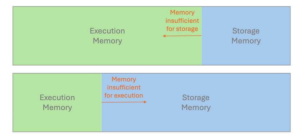
Spark uses Resilient Distributed Dataset (RDD) as its core building blocks, with data typically kept in memory by default. Whether executing computations (like joins and aggregations) or storing data across the cluster, all operations contribute to memory usage in a unified region.
A unified region with execution memory and storage memory (Image by author)
If we design improperly, the available memory may become insufficient. This causes excess partitions to spill onto the disk, which results in performance degradation.
Caching and persisting intermediate results or frequently accessed datasets are common practices. While both cache and persist serve the same purposes, they may differ in their storage levels. The resources should be used optimally to ensure efficient read and write operations.
For example, if transformed data will be reused repeatedly for computations and algorithms across different subsequent stages, it is advisable to cache that data.
Code example: Assume we want to investigate different subsets of transaction records using a digital wallet as the payment method.
After caching, even if we want to filter the transformed dataset with different transaction amount thresholds or other data dimensions, the execution times will still be more manageable.
#2 Shuffle
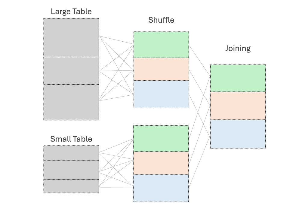
When we perform operations like joining DataFrames or grouping by data fields, shuffling occurs. This is necessary to redistribute all records across the cluster and to ensure those with the same key are on the same node. This in turn facilitates simultaneous processing and combining of the results.
Shuffle join (Image by author)
However, this shuffle operation is costly — high execution times and additional network overhead due to data movement between nodes.
To reduce shuffling, there are several strategies:
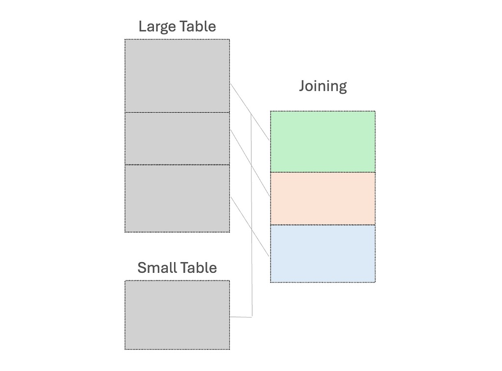
(1) Use broadcast variables for the small dataset, to send a read-only copy to every worker node for local processing
While “small” dataset is often defined by a maximum memory threshold of 8GB per executor, the ideal size for broadcasting should be determined through experimentation on specific case.
Broadcast join (Image by author)
(2) Early filtering, to minimize the amount of data processed as early as possible; and
(3) Control the number of partitions to ensure optimal performance
Code examples: Assume we want to return the transaction records that match our list of states, along with their full names
Inefficient — shuffle join between a large dataset and a small one
Data can sometimes be unevenly distributed, especially for data fields used as the key for processing. This leads to imbalanced partition sizes, in which some partitions are significantly larger or smaller than the average.
Since the execution performance is limited by the longest-running tasks, it is necessary to address the over-burdened nodes.
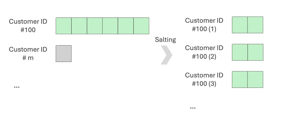
One common approach is salting. This works by adding randomized numbers to the skewed key so that there is a more uniform distribution across partitions. Let’s say when aggregating data based on the skewed key, we will aggregate using the salted key and then aggregate with the original key. Another method is re-partitioning, which increases the number of partitions to help distribute the data more evenly.
Data distribution — Before and after salting (Image by author)
Code examples: We want to aggregate an asymmetric dataset, mainly skewed by customer ID #100.
# Remove salt for further aggregation final_result = agg_data.withColumn("customerID", split(col("saltedCustomerID"), "_")[0]).groupBy("customerID").agg({"sum(totalAmt)": "sum"}).sort(desc("sum(sum(totalAmt))"))
return final_result
display(have_salting(df))
A random prefix or suffix to the skewed keys will both work. Generally, 5 to 10 random values are a good starting point to balance between spreading out the data and maintaining high complexity.
#4 Serialization
People often prefer using user-defined functions (UDFs) since it is flexible in customizing the data processing logic. However, UDFs operate on a row-by-row basis. The code shall be serialized by the Python interpreter, sent to the executor JVM, and then deserialized. This incurs high serialization costs and prevents Spark from optimizing and processing the code efficiently.
The simple and direct approach is to avoid using UDFs when possible.
We should first consider using the built-in Spark functions, which can handle tasks such as aggregation, arrays/maps operations, date/time stamps, and JSON data processing. If the built-in functions do not satisfy your desired tasks indeed, we can consider using pandas UDFs. They are built on top of Apache Arrow for lower overhead costs and higher performance, compared to UDFs.
Code examples: The transaction price is discounted based on the originating state.
Inefficient — using a UDF
from pyspark.sql.functions import udf from pyspark.sql.types import DoubleType from pyspark.sql import functions as F import numpy as np
# UDF to calculate discounted amount def calculate_discount(state, amount): if state == "CA": return amount * 0.90 # 10% off else: return amount * 0.85 # 15% off
@time_decorator def have_udf(data): # Use the UDF discounted_data = data.withColumn("discountedTotalAmt", discount_udf("state", "totalAmt"))
# Show the results return discounted_data.select("customerID", "totalAmt", "state", "discountedTotalAmt").show()
display(have_udf(df))
Efficient — using build-in PySpark functions
from pyspark.sql.functions import when

@time_decorator
def no_udf(data):
  # Use when and otherwise to discount the amount based on conditions
  discounted_data = data.withColumn(
  "discountedTotalAmt",
  when(data.state == "CA", data.totalAmt * 0.90)  # 10% off
  .otherwise(data.totalAmt * 0.85))  # 15% off

  # Show the results
  return discounted_data.select("customerID", "totalAmt", "state", "discountedTotalAmt").show()

display(no_udf(df))
In this example, we use the built-in PySpark functions “when and otherwise” to effectively check multiple conditions in sequence. There are unlimited examples based on our familiarity with those functions. For instance, pyspark.sql.functions.transforma function that aids in applying a transformation to each element in the input array has been introduced since PySpark version 3.1.0.
#5 Spill
As discussed in the Storage section, a spill occurs by writing temporary data from memory to disk due to insufficient memory to hold all the required data. Many performance issues we have covered are related to spills. For example, operations that shuffle large amounts of data between partitions can easily lead to memory exhaustion and subsequent spill.
Different scenarios of spill due to insufficient memory (Image by author)
It is crucial to examine the performance metrics in Spark UI. If we discover the statistics for Spill(Memory) and Spill(Disk), the spill is probably the reason for long-running tasks. To remediate this, try to instantiate a cluster with more memory per worker, e.g. increase the executor process size, by tuning the configuration value spark.executor.memory; Alternatively, we can configure spark.memory.fraction to adjust how much memory is allocated for execution and storage.
Wrapping it Up
We came across several common factors leading to performance degradation in PySpark, and the possible improvement methods:
Storage: use cache and persist to store the frequently used intermediate results
Shuffle: use broadcast variables for a small dataset to facilitate Spark’s local processing
Skewness: execute salting or repartitioning to distribute the skewed data more uniformly
Serialization: prefer to use built-in Spark functions to optimize the performance
Spill: adjust the configuration value to allocate memory wisely
Recently, Adaptive Query Execution (AQE) has been newly addressed for dynamic planning and re-planning of queries based on runtime stats. This supports different features of query re-optimization that occur during query execution, which creates a great optimization technique. However, understanding data characteristics during the initial design is still essential, as it informs better strategies for writing effective codes and queries while using AQE for fine-tuning.
Before you go
If you enjoy this reading, I invite you tofollow my Medium page and LinkedIn page. By doing so, you can stay updated with exciting content related to data science side projects, Machine Learning Operations (MLOps) demonstrations, and project management methodologies.
What exactly do you put in, what exactly do you get out, and how do you generate text with it?
Last week I was listening to an Acquired episode on Nvidia. The episode talks about transformers: the T in GPT and a candidate for the biggest invention of the 21st century.
Walking down Beacon Street, listening, I was thinking, I understand transformers, right? You mask out tokens during training, you have these attention heads that learn to connect concepts in text, you predict the probability of the next word. I’ve downloaded LLMs from Hugging Face and played with them. I used GPT-3 in the early days before the “chat” part was figured out. At Klaviyo we even built one of the first GPT-powered generative AI features in our subject line assistant. And way back I worked on a grammar checker powered by an older style language model. So maybe.
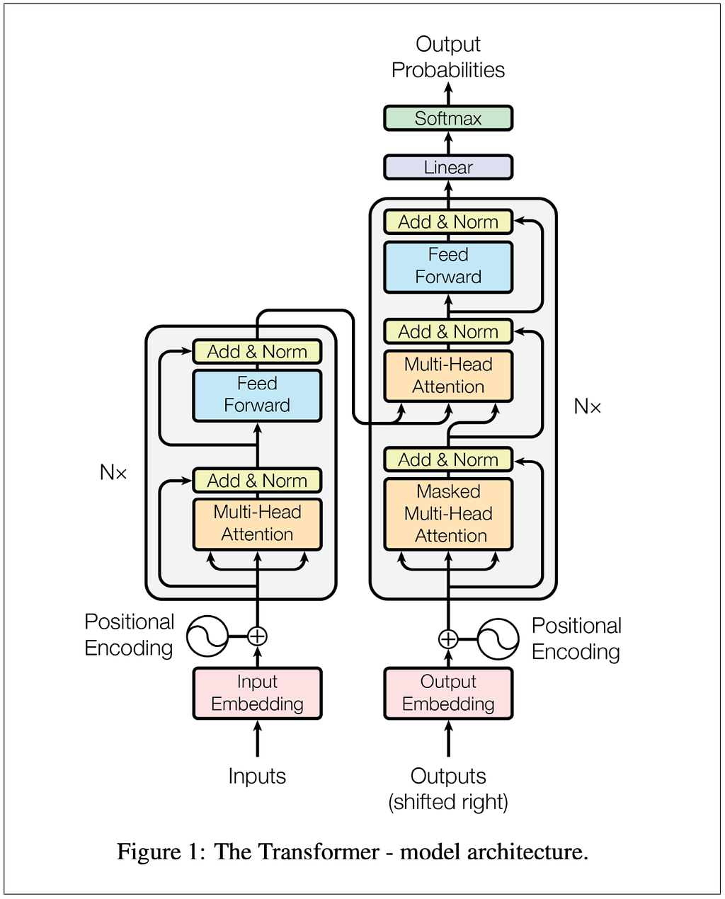
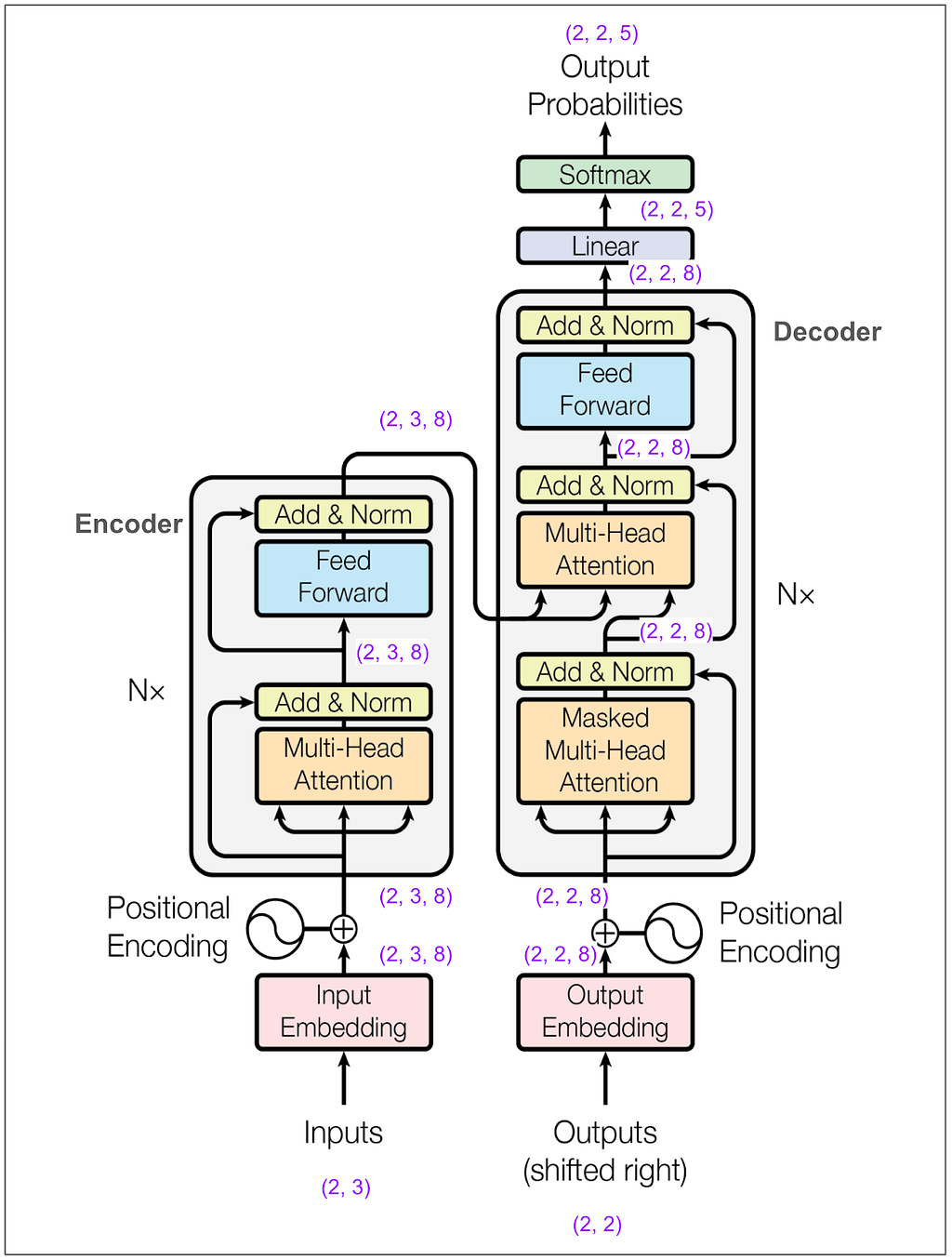
The transformer was invented by a team at Google working on automated translation, like from English to German. It was introduced to the world in 2017 in the now famous paper Attention Is All You Need. I pulled up the paper and looked at Figure 1:
Hmm…if I understood, it was only at the most hand-wavy level. The more I looked at the diagram and read the paper, the more I realized I didn’t get the details. Here are a few questions I wrote down:
During training, are the inputs the tokenized sentences in English and the outputs the tokenized sentences in German?
What exactly is each item in a training batch?
Why do you feed the output into the model and how is “masked multi-head attention” enough to keep it from cheating by learning the outputs from the outputs?
What exactly is multi-head attention?
How exactly is loss calculated? It can’t be that it takes a source language sentence, translates the whole thing, and computes the loss, that doesn’t make sense.
After training, what exactly do you feed in to generate a translation?
Why are there three arrows going into the multi-head attention blocks?
I’m sure those questions are easy and sound naive to two categories of people. The first is people who were already working with similar models (e.g. RNN, encoder-decoder) to do similar things. They must have instantly understood what the Google team accomplished and how they did it when they read the paper. The second is the many, many more people who realized how important transformers were these last seven years and took the time to learn the details.
Well, I wanted to learn, and I figured the best way was to build the model from scratch. I got lost pretty quickly and instead decided to trace code someone else wrote. I found this terrific notebook that explains the paper and implements the model in PyTorch. I copied the code and trained the model. I kept everything (inputs, batches, vocabulary, dimensions) tiny so that I could trace what was happening at each step. I found that noting the dimensions and the tensors on the diagrams helped me keep things straight. By the time I finished I had pretty good answers to all the questions above, and I’ll get back to answering them after the diagrams.
Here are cleaned up versions of my notes. Everything in this part is for training one single, tiny batch, which means all the tensors in the different diagrams go together.
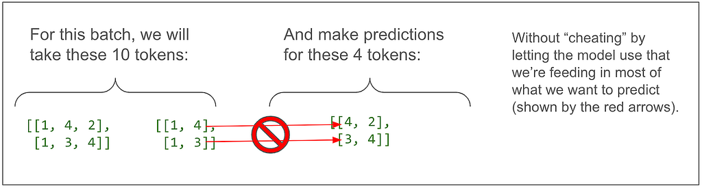
To keep things easy to follow, and copying an idea from the notebook, we’re going to train the model to copy tokens. For example, once trained, “dog run” should translate to “dog run”.
In other words:
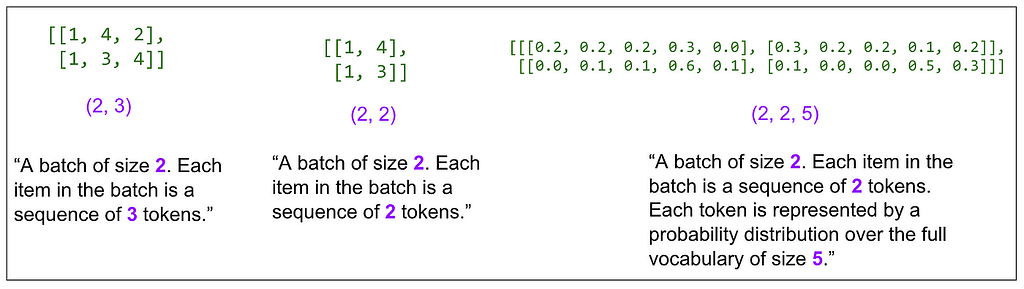
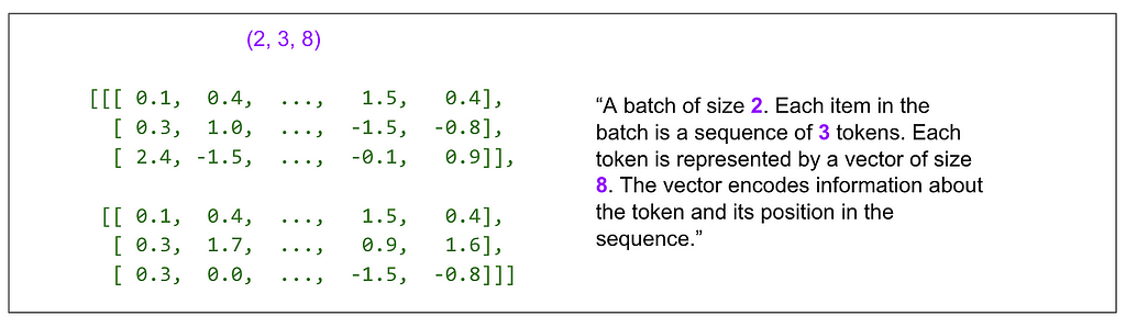
And here’s trying to put into words what the tensor dimensions (shown in purple) on the diagram so far mean:
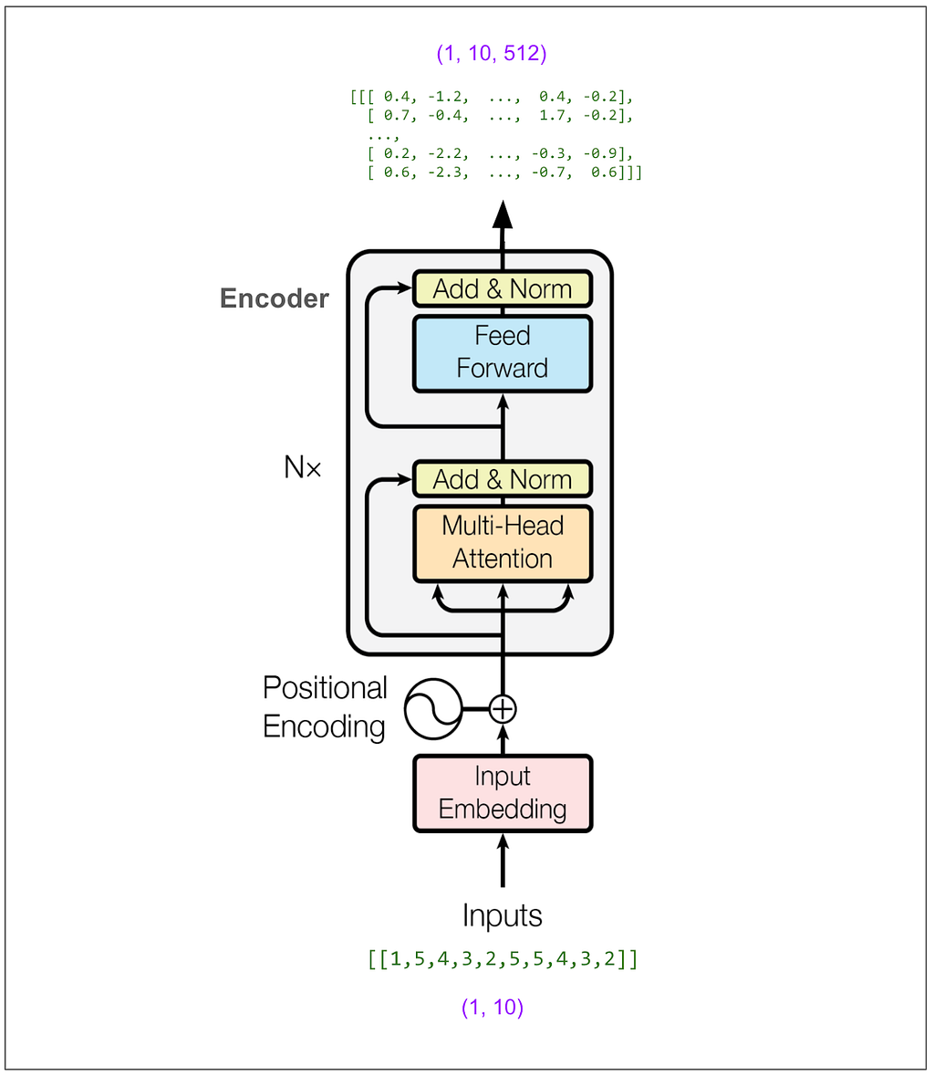
One of the hyperparameters is d-model and in the base model in the paper it’s 512. In this example I made it 8. This means our embedding vectors have length 8. Here’s the main diagram again with dimensions marked in a bunch of places:
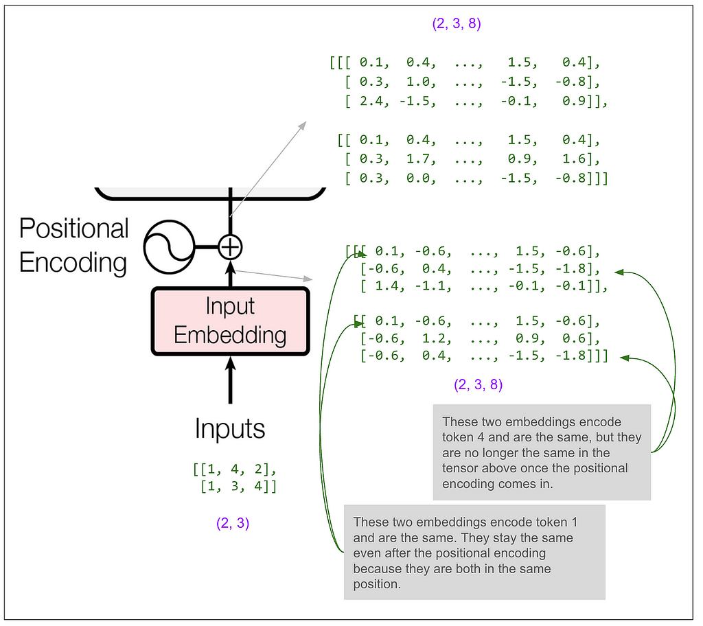
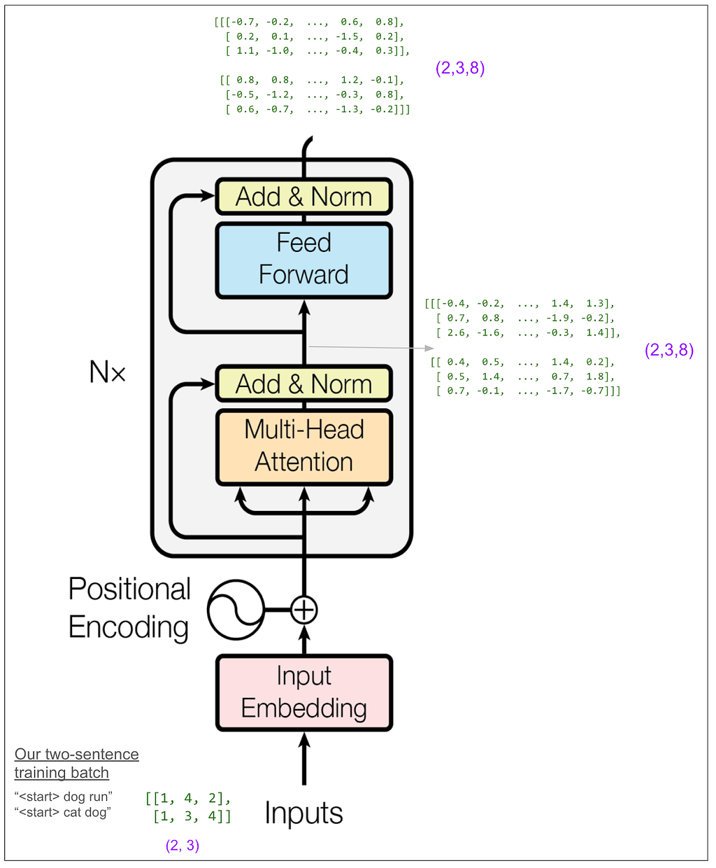
Let’s zoom in on the input to the encoder:
Most of the blocks shown in the diagram (add & norm, feed forward, the final linear transformation) act only on the last dimension (the 8). If that’s all that was happening then the model would only get to use the information in a single position in the sequence to predict a single position. Somewhere it must get to “mix things up” among positions and that magic happens in the multi-head attention blocks.
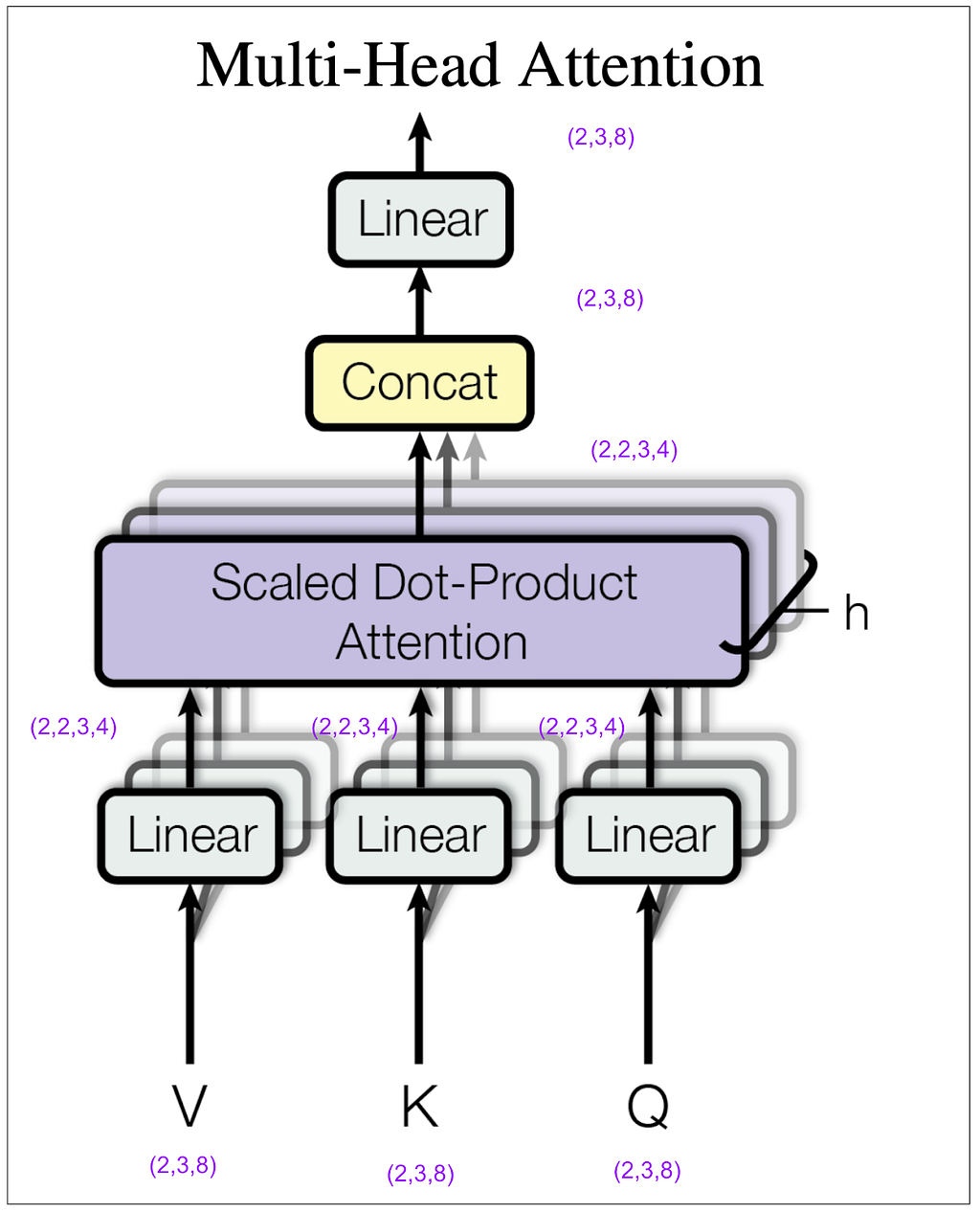
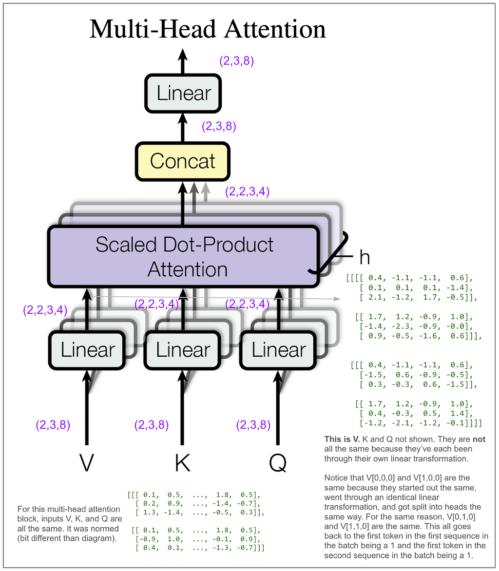
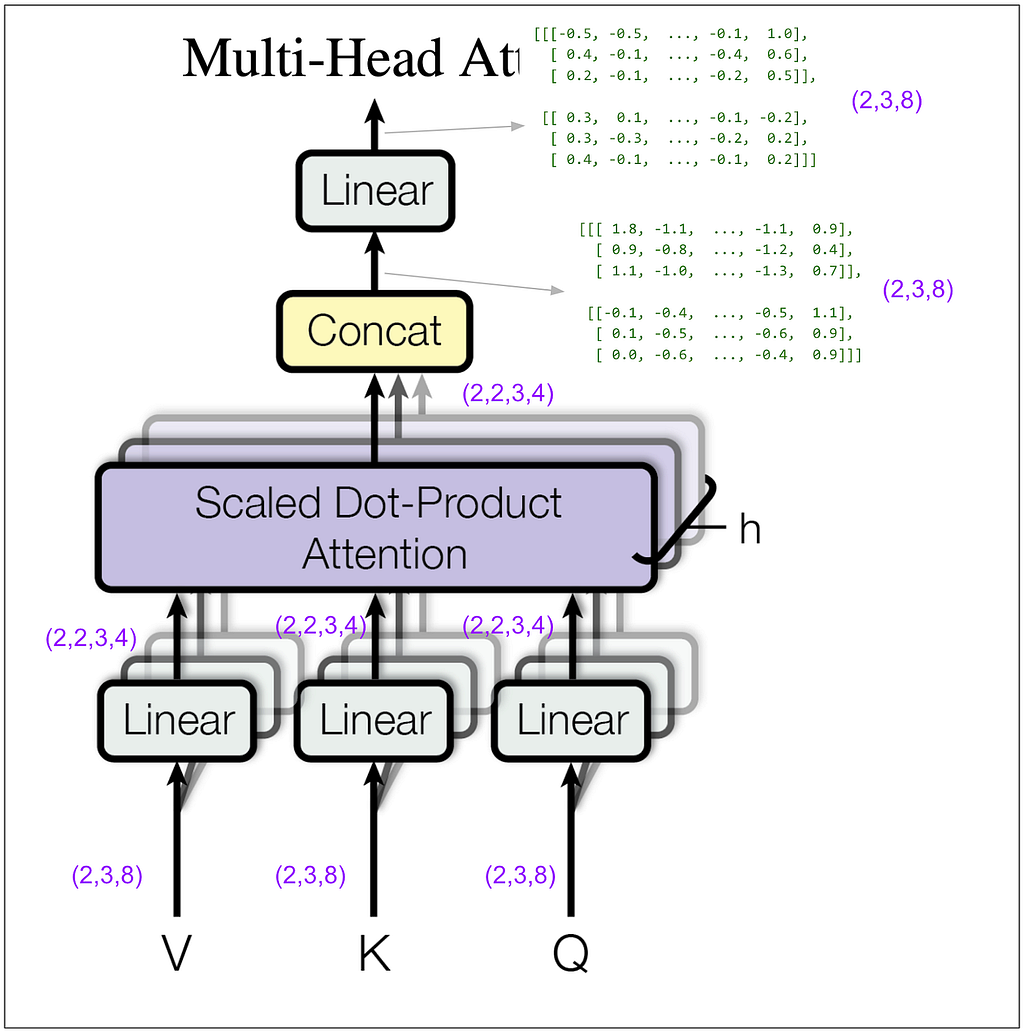
Let’s zoom in on the multi-head attention block within the encoder. For this next diagram, keep in mind that in my example I set the hyperparameter h (number of heads) to 2. (In the base model in the paper it’s 8.)
How did (2,3,8) become (2,2,3,4)? We did a linear transformation, then took the result and split it into number of heads (8 / 2 = 4) and rearranged the tensor dimensions so that our second dimension is the head. Let’s look at some actual tensors:
We still haven’t done anything that mixes information among positions. That’s going to happen next in the scaled dot-product attention block. The “4” dimension and the “3” dimension will finally touch.
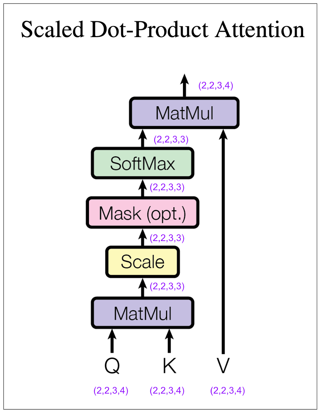
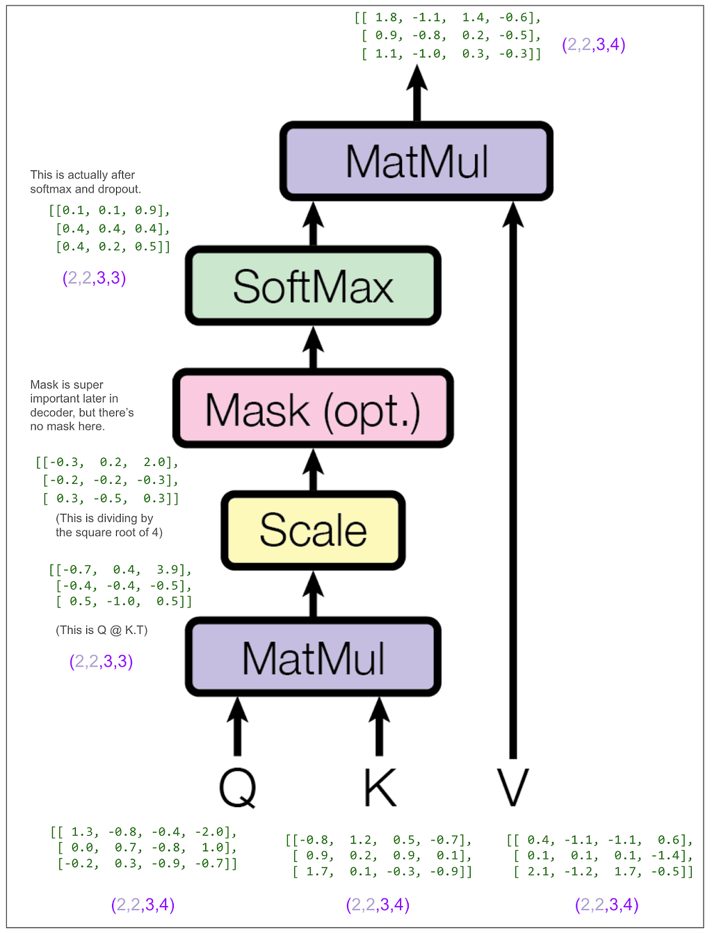
Let’s look at the tensors, but to make it easier to follow, we’ll look only at the first item in the batch and the first head. In other words, Q[0,0], K[0,0], etc. The same thing will be happening to the other three.
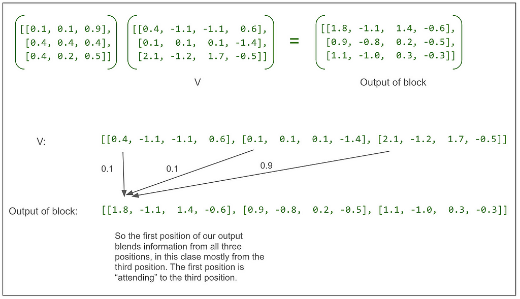
Let’s look at that final matrix multiplication between the output of the softmax and V:
Following from the very beginning, we can see that up until that multiplication, each of the three positions in V going all the way back to our original sentence “<start> dog run” has only been operated on independently. This multiplication blends in information from other positions for the first time.
Going back to the multi-head attention diagram, we can see that the concat puts the output of each head back together so each position is now represented by a vector of length 8. Notice that the 1.8 and the -1.1 in the tensor after concat but before linear match the 1.8 and -1.1 from the first two elements in the vector for the first position of the first head in the first item in the batch from the output of the scaled dot-product attention shown above. (The next two numbers match too but they’re hidden by the ellipses.)
Now let’s zoom back out to the whole encoder:
At first I thought I would want to trace the feed forward block in detail. It’s called a “position-wise feed-forward network” in the paper and I thought that meant it might bring information from one position to positions to the right of it. However, it’s not that. “Position-wise” means that it operates independently on each position. It does a linear transform on each position from 8 elements to 32, does ReLU (max of 0 and number), then does another linear transform to get back to 8. (That’s in our small example. In the base model in the paper it goes from 512 to 2048 and then back to 512. There are a lot of parameters here and probably this is where a lot of the learning happens!) The output of the feed forward is back to (2,3,8).
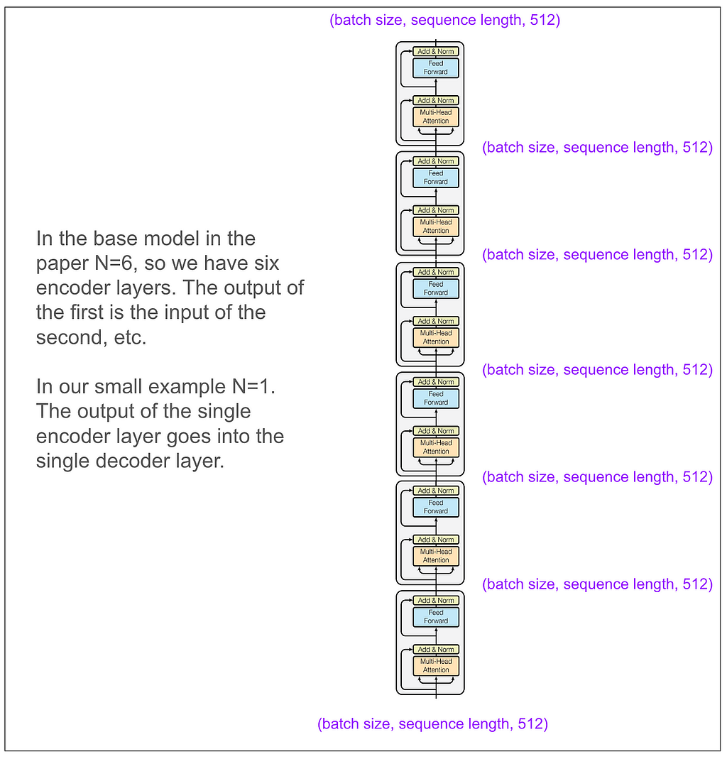
Getting away from our toy model for a second, here’s how the encoder looks in the base model in the paper. It’s very nice that the input and output dimensions match!
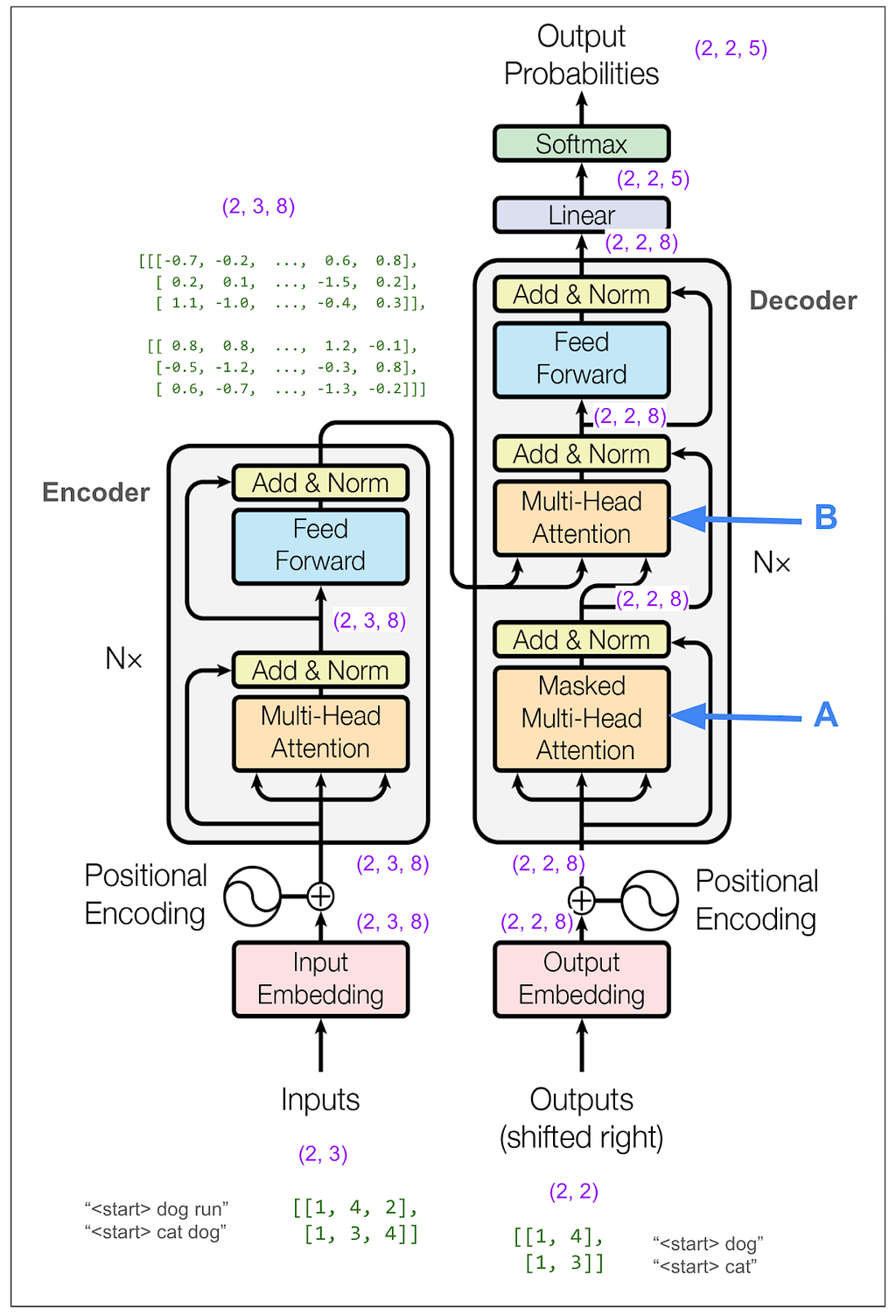
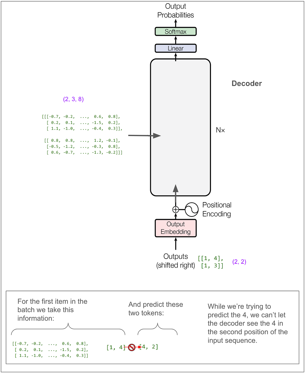
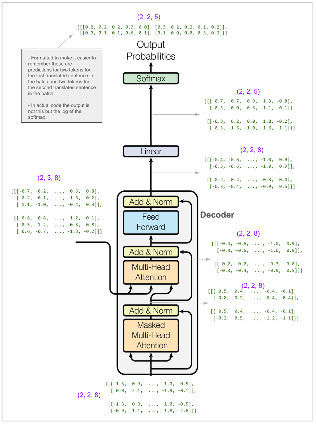
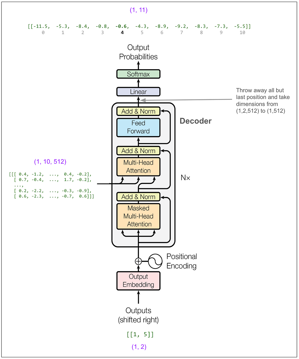
Now let’s zoom out all the way so we can look at the decoder.
We don’t need to trace most of the decoder side because it’s very similar to what we just looked at on the encoder side. However, the parts I labeled A and B are different. A is different because we do masked multi-head attention. This must be where the magic happens to not “cheat” while training. B we’ll come back to later. But first let’s hide the internal details and keep in mind the big picture of what we want to come out of the decoder.
And just to really drive home this point, suppose our English sentence is “she pet the dog” and our translated Pig Latin sentence is “eshay etpay ethay ogday”. If the model has “eshay etpay ethay” and is trying to come up with the next word, “ogday” and “atcay” are both high probability choices. Given the context of the full English sentence of “she pet the dog,” it really should be able to choose “ogday.” However, if the model could see the “ogday” during training, it wouldn’t need to learn how to predict using the context, it would just learn to copy.
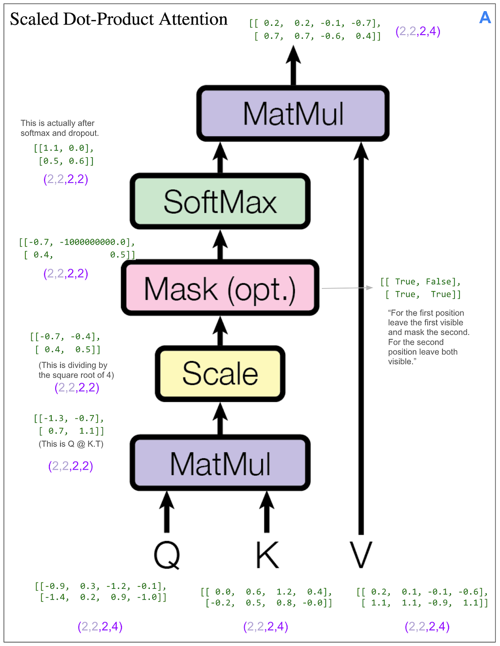
Let’s see how the masking does this. We can skip ahead a bit because the first part of A works exactly the same as before where it applies linear transforms and splits things up into heads. The only difference is the dimensions coming into the scaled dot-product attention part are (2,2,2,4) instead of (2,2,3,4) because our original input sequence is of length two. Here’s the scaled dot-product attention part. As we did on the encoder side, we’re looking at only the first item in the batch and the first head.
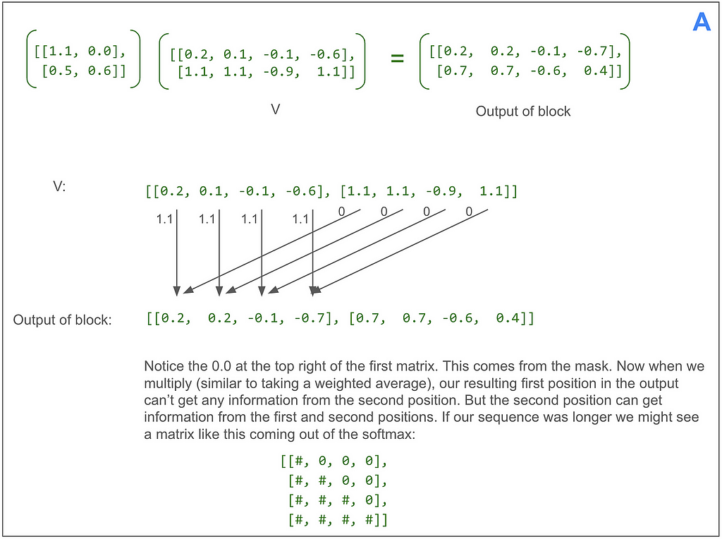
This time we have a mask. Let’s look at the final matrix multiplication between the output of the softmax and V:
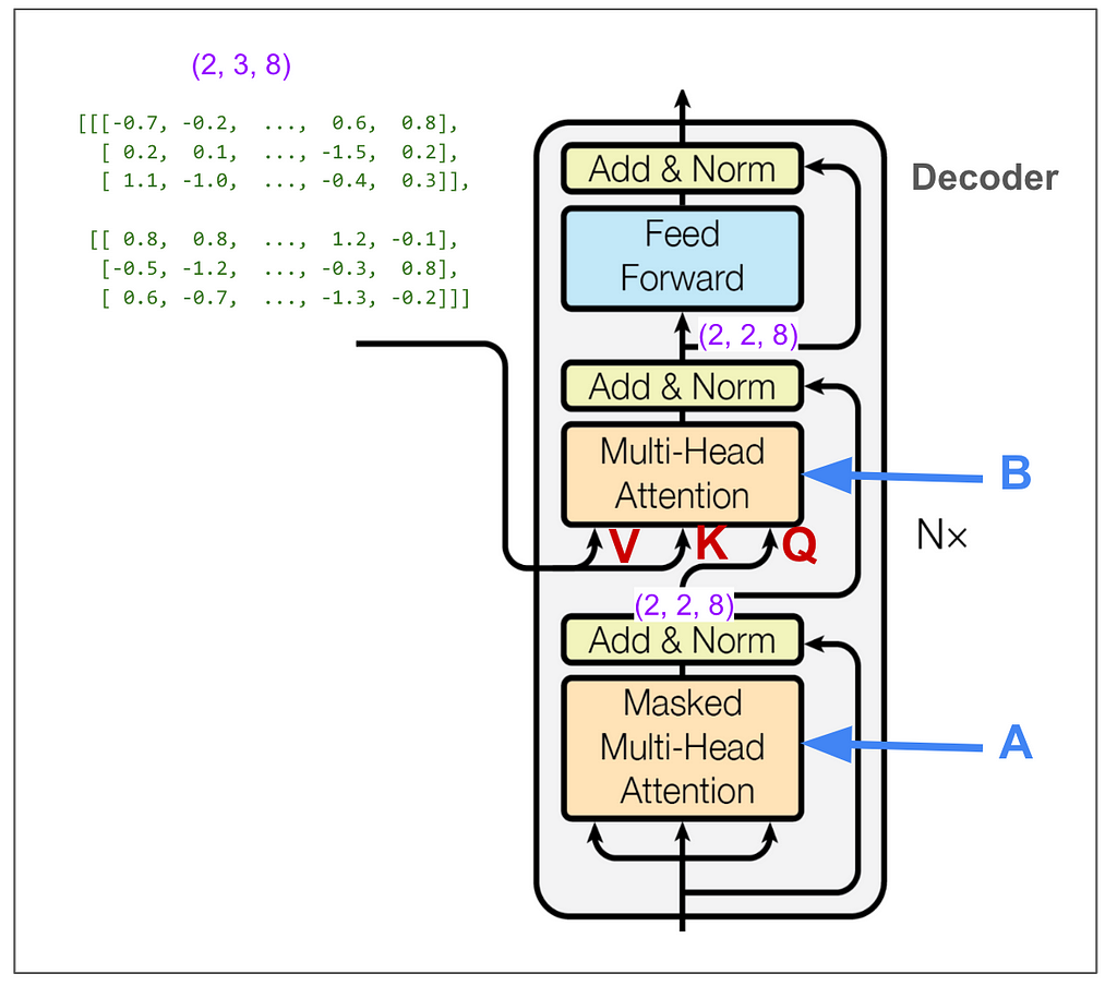
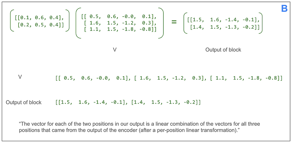
Now we’re ready to look at B, the second multi-head attention in the decoder. Unlike the other two multi-head attention blocks, we’re not feeding in three identical tensors, so we need to think about what’s V, what’s K and what’s Q. I labeled the inputs in red. We can see that V and K come from the output of the encoder and have dimension (2,3,8). Q has dimension (2,2,8).
As before, we skip ahead to the scaled dot-product attention part. It makes sense, but is also confusing, that V and K have dimensions (2,2,3,4) — two items in the batch, two heads, three positions, vectors of length four, and Q has dimension (2,2,2,4).
Even though we’re “reading from” the encoder output where the “sequence” length is three, somehow all the matrix math works out and we end up with our desired dimension (2,2,2,4). Let’s look at the final matrix multiplication:
The outputs of each multi-head attention block get added together. Let’s skip ahead to see the output from the decoder and turning that into predictions:
The linear transform takes us from (2,2,8) to (2,2,5). Think about that as reversing the embedding, except that instead of going from a vector of length 8 to the integer identifier for a single token, we go to a probability distribution over our vocabulary of 5 tokens. The numbers in our tiny example make that seem a little funny. In the paper, it’s more like going from a vector of size 512 to a vocabulary of 37,000 when they did English to German.
In a moment we’ll calculate the loss. First, though, even at a glance, you can get a feel for how the model is doing.
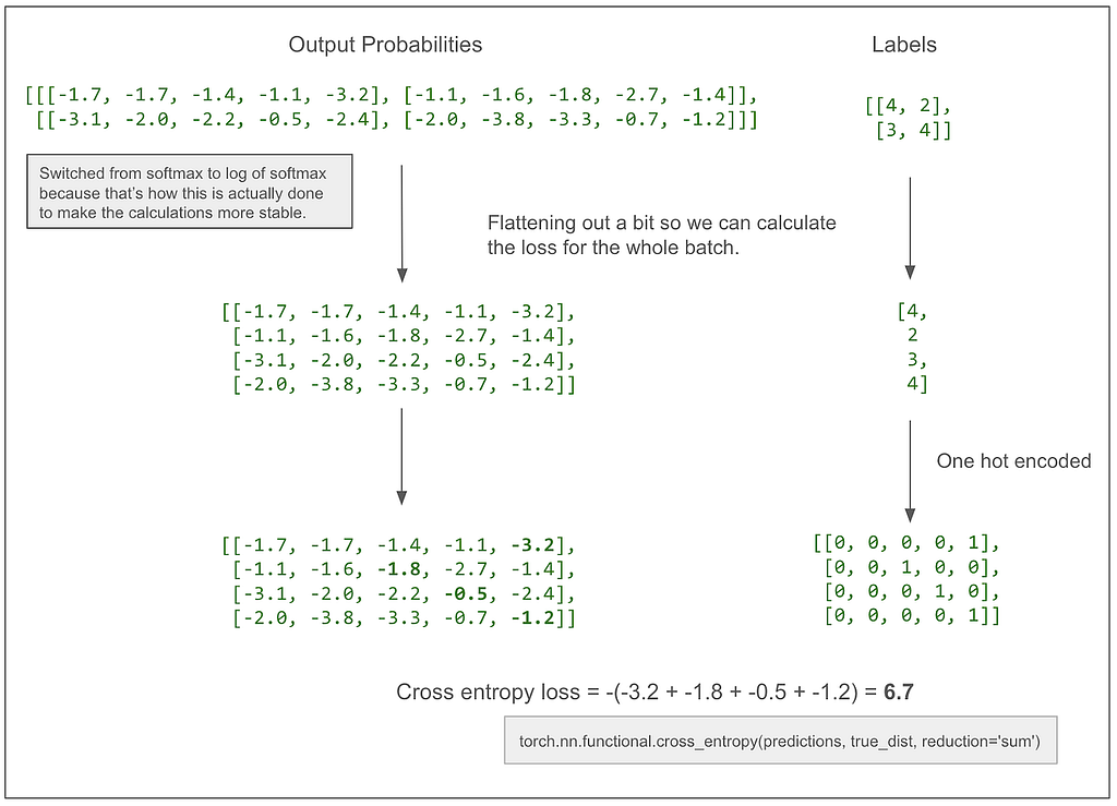
It got one token right. No surprise because this is our first training batch and it’s all just random. One nice thing about this diagram is it makes clear that this is a multi-class classification problem. The classes are the vocabulary (5 classes in this case) and, this is what I was confused about before, we make (and score) one prediction per token in the translated sentence, NOT one prediction per sentence. Let’s do the actual loss calculation.
If, for example, the -3.2 became a -2.2, our loss would decrease to 5.7, moving in the desired direction, because we want the model to learn that the correct prediction for that first token is 4.
The diagram above leaves out label smoothing. In the actual paper, the loss calculation smooths labels and uses KL Divergence loss. I think that works out to be the same or simialr to cross entropy when there is no smoothing. Here’s the same diagram as above but with label smoothing.
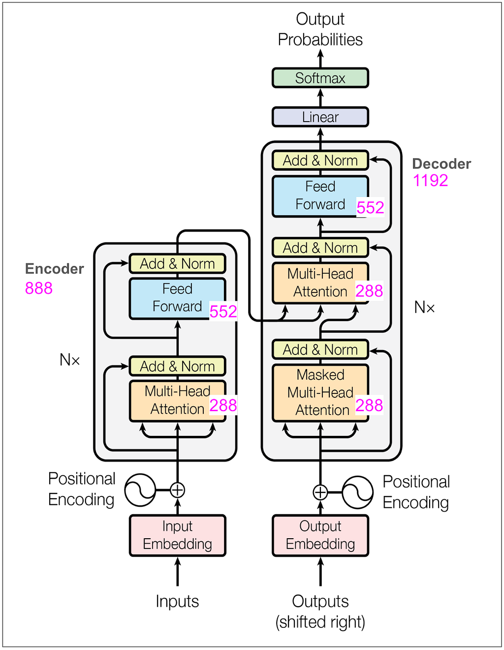
Let’s also take a quick look at the number of parameters being learned in the encoder and decoder:
As a sanity check, the feed forward block in our toy model has a linear transformation from 8 to 32 and back to 8 (as explained above) so that’s 8 * 32 (weights) + 32 (bias) + 32 * 8 (weights) + 8 (bias) = 52. Keep in mind that in the base model in the paper, where d-model is 512 and d-ff is 2048 and there are 6 encoders and 6 decoders there will be many more parameters.
Using the trained model
Now let’s see how we put source language text in and get translated text out. I’m still using a toy model here trained to “translate” by coping tokens, but instead of the example above, this one uses a vocabulary of size 11 and d-model is 512. (Above we had vocabulary of size 5 and d-model was 8.)
First let’s do a translation. Then we’ll see how it works.
Step one is to feed the source sentence into the encoder and hold onto its output, which in this case is a tensor with dimensions (1, 10, 512).
Step two is to feed the first token of the output into the decoder and predict the second token. We know the first token because it’s always <start> = 1.
In the paper, they use beam search with a beam size of 4, which means we would consider the 4 highest probability tokens at this point. To keep things simple I’m going to instead use greedy search. You can think of that as a beam search with a beam size of 1. So, reading off from the top of the diagram, the highest probability token is number 5. (The outputs above are logs of probabilities. The highest probability is still the highest number. In this case that’s -0.0 which is actually -0.004 but I’m only showing one decimal place. The model is really confident that 5 is correct! exp(-0.004) = 99.6%)
Now we feed [1,5] into the decoder. (If we were doing beam search with a beam size of 2, we could instead feed in a batch containing [1,5] and [1,4] which is the next most likely.)
Now we feed [1,5,4]:
And get out 3. And so on until we get a token that indicates the end of the sentence (not present in our example vocabulary) or hit a maximum length.
Circling back to the questions above
Now I can mostly answer my original questions.
During training, are the inputs the tokenized sentences in English and the outputs the tokenized sentences in German?
Yes, more or less.
What exactly is each item in a training batch?
Each item corresponds to one translated sentence pair.
The “x” of the item has two parts. The first part is all the tokens of the source sentence. The second part is all tokens of the target sentence except for the last one.
The “y” (label) of the item is all tokens of the target sentence except for the first one. Since the first token for source and target is always <start>, we’re not wasting or losing any training data.
What’s a little subtle is that if this were a classification task where say the model had to take an image and output a class (house, car, rabbit, etc.), we would think of each item in the batch as contributing one “classification” to the loss calculation. Here, however, each item in the batch will contribute (number_of_tokens_in_target_sentence — 1) “classifications” to the loss calculation.
Why do you feed the output into the model and how is “masked multi-head attention” enough to keep it from cheating by learning the outputs from the outputs?
You feed the output so the model can learn to predict the translation based both on the meaning of the source sentence and the words translated so far. Although lots of things are going on in the model, the only time information moves between positions is during the attention steps. Although we do feed the translated sentence into the decoder, the first attention calculation uses a mask to zero out all information from positions beyond the one we’re predicting.
What exactly is multi-head attention?
I probably should have asked what exactly is attention, because that’s the more central concept. Multi-head attention means slicing the vectors up into groups, doing attention on the groups, and then putting the groups back together. For example, if the vectors have size 512 and there are 8 heads, attention will be done independently on 8 groups each containing a full batch of the full positions, each position having a vector of size 64. If you squint, you can see how each head could end up learning to give attention to certain connected concepts as in the famous visualizations showing how a head will learn what word a pronoun references.
How exactly is loss calculated? It can’t be that it takes a source language sentence, translates the whole thing, and computes the loss, that doesn’t make sense.
Right. We’re not translating a full sentence in one go and calculating overall sentence similarity or something like that. Loss is calculated just like in other multi-class classification problems. The classes are the tokens in our vocabulary. The trick is we’re independently predicting a class for every token in the target sentence using only the information we should have at that point. The labels are the actual tokens from our target sentence. Using the predictions and labels we calculate loss using cross entropy. (In reality we “smooth” our labels to account for the fact that they’re notabsolute, a synonym could sometimes work equally well.)
After training, what exactly do you feed in to generate a translation?
You can’t feed something in and have the model spit out the translation in a single evaluation. You need to use the model multiple times. You first feed the source sentence into the encoder part of the model and get an encoded version of the sentence that represents its meaning in some abstract, deep way. Then you feed that encoded information and the start token <start> into the decoder part of the model. That lets you predict the second token in the target sentence. Then you feed in the <start> and second token to predict the third. You repeat this until you have a full translated sentence. (In reality, though, you consider multiple high probability tokens for each position, feed multiple candidate sequences in each time, and pick the final translated sentence based on total probability and a length penalty.)
Why are there three arrows going into the multi-head attention blocks?
I’m guessing three reasons. 1) To show that the second multi-head attention block in the decoder gets some of its input from the encoder and some from the prior block in the decoder. 2) To hint at how the attention algorithm works. 3) To hint that each of the three inputs undergoes its own independent linear transformation before the actual attention happens.
Conclusion
It’s beautiful! I probably wouldn’t think that if it weren’t so incredibly useful. I now get the feeling people must have had when they first saw this thing working. This elegant and trainable model expressible in very little code learned how to translate human languages and beat out complicated machine translations systems built over decades. It’s amazing and clever and unbelievable. You can see how the next step was to say, forget about translated sentence pairs, let’s use this technique on every bit of text on the internet — and LLMs were born!
(I bet have some mistakes above. Please LMK.)
Unless otherwise noted, all images are by author, or contain annotations by the author on figures from Attention Is All You Need.
Spark Connect is a relatively new component in the Spark ecosystem that allows thin clients to run Spark applications on a remote Spark cluster. This technology can offer some benefits to Spark applications that use the DataFrame API. Spark has long allowed to run SQL queries on a remote Thrift JDBC server. However, this ability to remotely run client applications written in any supported language (Scala, Python) appeared only in Spark 3.4.
In this article, I will share our experience using Spark Connect (version 3.5). I will talk about the benefits we gained, technical details related to running Spark client applications, and some tips on how to make your Spark Connect setup more efficient and stable.
Motivation for use
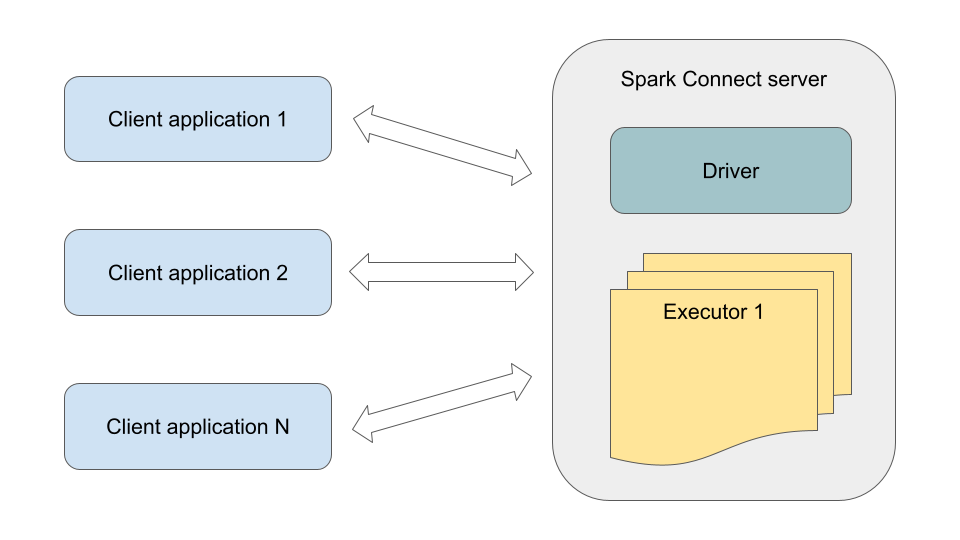
Spark is one of the key components of the analytics platform at Joom. We have a large number of internal users and over 1000 custom Spark applications. These applications run at different times of day, have different complexity, and require very different amounts of computing resources (ranging from a few cores for a couple of minutes to over 250 cores for several days). Previously, all of them were always executed as separate Spark applications (with their own driver and executors), which, in the case of small and medium-sized applications (we historically have many such applications), led to noticeable overhead. With the introduction of Spark Connect, it is now possible to set up a shared Spark Connect server and run many Spark client applications on it. Technically, the Spark Connect server is a Spark application with an embedded Spark Connect endpoint.
Image by author
Here are the benefits we were able to get from this:
Resource savings – When running via Spark Connect, client applications do not require their own Spark driver (which typically uses over 1.5 GB of memory). Instead, they use a thin client with a typical memory consumption of 200 MB. – Executor utilization improves since any executor can run the tasks of multiple client applications. For example, suppose some Spark application, at some point in its execution, starts using significantly fewer cores and memory than initially requested. There are many reasons why this can happen. Then, in the case of a separate Spark application, currently unused resources are often wasted since dynamic allocation often does not provide efficient scale-down. However, with the Spark Connect server, the freed-up cores and memory can immediately be used to run tasks of other client applications.
Reduced startup wait time – For various reasons, we have to limit the number of simultaneously running separate Spark applications, and they may wait in the queue for quite a long time if all slots are currently occupied. It can negatively affect data readiness time and user experience. In the case of the Spark Connect server, we have so far been able to avoid such limitations, and all Spark Connect client applications start running immediately after launch. – For ad-hoc executions, it is desirable to minimize the time to get results as much as possible and avoid keeping people waiting. In the case of separate Spark applications, launching a client application often requires provisioning additional EC2 nodes for its driver and executors, as well as initializing the driver and executors. All of this together can take more than 4 minutes. In the case of the Spark Connect server, at least its driver is always up and ready to accept requests, so it is only a matter of waiting for additional executors, and often executors are already available. This may significantly reduce the wait time for ad-hoc applications to be ready.
Our constraints
At the moment, we do not run long-running heavy applications on Spark Connect for the following reasons:
They may cause failure or unstable behavior of the Spark Connect server (e.g., by overflowing disks on executor nodes). It can lead to large-scale problems for the entire platform.
They often require unique memory settings and use specific optimization techniques (e.g., custom extraStrategies).
We currently have a problem with giving the Spark Connect server a lot of executors to handle a very large simultaneous load (this is related to the behavior of Spark Task Scheduler and is beyond the scope of this article).
Therefore, heavy applications still run as separate Spark applications.
We have too many different, constantly changing Spark applications, and it would take too much time to manually determine for each one whether it should run on Spark Connect according to our criteria or not. Furthermore, the list of applications running on Spark Connect needs to be updated regularly. For example, suppose today, some application is light enough, so we have decided to run it on Spark Connect. But tomorrow, its developers may add several large joins, making it quite heavy. Then, it will be preferable to run it as a separate Spark application. The reverse situation is also possible.
Eventually, we created a service to automatically determine how to launch each specific client application. This service analyzes the history of previous runs for each application, evaluating such metrics as Total Task Time, Shuffle Write, Disk Spill, and others (this data is collected using SparkListener). Custom parameters set for the applications by developers (e.g., memory settings of drivers and executors) are also considered. Based on this data, the service automatically determines for each application whether it should be run this time on the Spark Connect server or as a separate Spark application. Thus, all our applications should be ready to run in either of the two ways.
In our environment, each client application is built independently of the others and has its own JAR file containing the application code, as well as specific dependencies (for example, ML applications often use third-party libraries like CatBoost and so on). The problem is that the SparkSession API for Spark Connect is somewhat different from the SparkSession API used for separate Spark applications (Spark Connect clients use the spark-connect-client-jvm artifact). Therefore, we are supposed to know at the build time of each client application whether it will run via Spark Connect or not. But we do not know that. The following describes our approach to launching client applications, which eliminates the need to build and manage two versions of JAR artifact for the same application.
For each Spark client application, we build only one JAR file containing the application code and specific dependencies. This JAR is used both when running on Spark Connect and when running as a separate Spark application. Therefore, these client JARs do not contain specific Spark dependencies. The appropriate Spark dependencies (spark-core/spark-sql or spark-connect-client-jvm) will be provided later in the Java classpath, depending on the run mode. In any case, all client applications use the same Scala code to initialize SparkSession, which operates depending on the run mode. All client application JARs are built for the regular Spark API. So, in the part of the code intended for Spark Connect clients, the SparkSession methods specific to the Spark Connect API (remote, addArtifact) are called via reflection:
val sparkConnectUri: Option[String] = Option(System.getenv("SPARK_CONNECT_URI"))
val isSparkConnectMode: Boolean = sparkConnectUri.isDefined
def createSparkSession(): SparkSession = { if (isSparkConnectMode) { createRemoteSparkSession() } else { SparkSession.builder // Whatever you need to do to configure SparkSession for a separate // Spark application. .getOrCreate } }
private def createRemoteSparkSession(): SparkSession = { val uri = sparkConnectUri.getOrElse(throw new Exception( "Required environment variable 'SPARK_CONNECT_URI' is not set."))
val builder = SparkSession.builder // Reflection is used here because the regular SparkSession API does not // contain these methods. They are only available in the SparkSession API // version for Spark Connect. classOf[SparkSession.Builder] .getDeclaredMethod("remote", classOf[String]) .invoke(builder, uri)
// A set of identifiers for this application (to be used later). val scAppId = s"spark-connect-${UUID.randomUUID()}" val airflowTaskId = Option(System.getenv("AIRFLOW_TASK_ID")) .getOrElse("unknown_airflow_task_id") val session = builder .config("spark.joom.scAppId", scAppId) .config("spark.joom.airflowTaskId", airflowTaskId) .getOrCreate()
// If the client application uses your Scala code (e.g., custom UDFs), // then you must add the jar artifact containing this code so that it // can be used on the Spark Connect server side. val addArtifact = Option(System.getenv("ADD_ARTIFACT_TO_SC_SESSION")) .forall(_.toBoolean)
if (addArtifact) { val mainApplicationFilePath = System.getenv("SPARK_CONNECT_MAIN_APPLICATION_FILE_PATH") classOf[SparkSession] .getDeclaredMethod("addArtifact", classOf[String]) .invoke(session, mainApplicationFilePath) }
In the case of Spark Connect mode, this client code can be run as a regular Java application anywhere. Since we use Kubernetes, this runs in a Docker container. All dependencies specific to Spark Connect are packed into a Docker image used to run client applications (a minimal example of this image can be found here). The image contains not only the spark-connect-client-jvm artifact but also other common dependencies used by almost all client applications (e.g., hadoop-aws since we almost always have interaction with S3 storage on the client side).
FROM openjdk:11-jre-slim

WORKDIR /app

# Here, we copy the common artifacts required for any of our Spark Connect
# clients (primarily spark-connect-client-jvm, as well as spark-hive,
# hadoop-aws, scala-library, etc.).
COPY build/libs/* /app/

COPY src/main/docker/entrypoint.sh /app/
RUN chmod +x ./entrypoint.sh
ENTRYPOINT ["./entrypoint.sh"]
This common Docker image is used to run all our client applications when it comes to running them via Spark Connect. At the same time, it does not contain client JARs with the code of particular applications and their dependencies because there are many such applications that are constantly updated and may depend on any third-party libraries. Instead, when a particular client application is launched, the location of its JAR file is passed using an environment variable, and that JAR is downloaded during initialization in entrypoint.sh:
#!/bin/bash
set -eo pipefail

# This variable will also be used in the SparkSession builder within
# the application code.
export SPARK_CONNECT_MAIN_APPLICATION_FILE_PATH="/tmp/$(uuidgen).jar"

# Download the JAR with the code and specific dependencies of the client
# application to be run. All such JAR files are stored in S3, and when
# creating a client Pod, the path to the required JAR is passed to it
# via environment variables.
java -cp "/app/*" com.joom.analytics.sc.client.S3Downloader
    ${MAIN_APPLICATION_FILE_S3_PATH} ${SPARK_CONNECT_MAIN_APPLICATION_FILE_PATH}

# Launch the client application. Any MAIN_CLASS initializes a SparkSession
# at the beginning of its execution using the code provided above.
java -cp ${SPARK_CONNECT_MAIN_APPLICATION_FILE_PATH}:"/app/*" ${MAIN_CLASS} "$@"
Finally, when it comes time to launch the application, our custom SparkAirflowOperator automatically determines the execution mode (Spark Connect or separate) based on the statistics of previous runs of this application.
In the case of Spark Connect, we use KubernetesPodOperator to launch the client Pod of the application. KubernetesPodOperator takes as parameters the previously described Docker image, as well as the environment variables (MAIN_CLASS, JAR_PATH and others), which will be available for use within entrypoint.sh and the application code. There is no need to allocate many resources to the client Pod (for example, its typical consumption in our environment: memory — 200 MB, vCPU — 0.15).
In the case of a separate Spark application, we use our custom AirflowOperator, which runs Spark applications using spark-on-k8s-operator and the official Spark Docker image. Let’s skip the details about our Spark AirflowOperator for now, as it is a large topic deserving a separate article.
Compatibility issues with regular Spark applications
Not all existing Spark applications can be successfully executed on Spark Connect since its SparkSession API is different from the SparkSession API used for separate Spark applications. For example, if your code uses sparkSession.sparkContext or sparkSession.sessionState, it will fail in the Spark Connect client because the Spark Connect version of SparkSession does not have these properties.
In our case, the most common cause of problems was using sparkSession.sessionState.catalog and sparkSession.sparkContext.hadoopConfiguration. In some cases, sparkSession.sessionState.catalog can be replaced with sparkSession.catalog, but not always. sparkSession.sparkContext.hadoopConfiguration may be needed if the code executed on the client side contains operations on your data storage, such as this:
Fortunately, it is possible to create a standalone SessionCatalog for use within the Spark Connect client. In this case, the class path of the Spark Connect client must also include org.apache.spark:spark-hive_2.12, as well as libraries for interacting with your storage (since we use S3, so in our case, it is org.apache.hadoop:hadoop-aws).
// This is just an example of what the required properties might look like. // All of them should already be set for existing Spark applications in one // way or another, and their complete list can be found in the UI of any // running separate Spark application on the Environment tab. val sessionCatalogConfig = Map( "spark.hadoop.hive.metastore.uris" -> "thrift://metastore.spark:9083", "spark.sql.catalogImplementation" -> "hive", "spark.sql.catalog.spark_catalog" -> "org.apache.spark.sql.delta.catalog.DeltaCatalog", )
val hadoopConfig = Map( "hive.metastore.uris" -> "thrift://metastore.spark:9083", "fs.s3.impl" -> "org.apache.hadoop.fs.s3a.S3AFileSystem", "fs.s3a.aws.credentials.provider" -> "com.amazonaws.auth.DefaultAWSCredentialsProviderChain", "fs.s3a.endpoint" -> "s3.amazonaws.com", // and others... )
def createStandaloneSessionCatalog(): (SessionCatalog, Configuration) = { val sparkConf = new SparkConf().setAll(sessionCatalogConfig) val hadoopConfiguration = new Configuration() hadoopConfig.foreach { case (key, value) => hadoopConfiguration.set(key, value) }
val externalCatalog = new StandaloneHiveExternalCatalog( sparkConf, hadoopConfiguration) val sessionCatalog = new SessionCatalog( new ExternalCatalogWithListener(externalCatalog) ) (sessionCatalog, hadoopConfiguration) }
You also need to create a wrapper for HiveExternalCatalog accessible in your code (because the HiveExternalCatalog class is private to the org.apache.spark package):
Unfortunately, it is not always easy to fix a particular Spark application to make it work as a Spark Connect client. For example, third-party Spark components used in the project pose a significant risk, as they are often written without considering compatibility with Spark Connect. Since, in our environment, any Spark application can be automatically launched on Spark Connect, we found it reasonable to implement a fallback to a separate Spark application in case of failure. Simplified, the logic is as follows:
If some application fails on Spark Connect, we immediately try to rerun it as a separate Spark application. At the same time, we increment the counter of failures that occurred during execution on Spark Connect (each client application has its own counter).
The next time this application is launched, we check the failure counter of this application: – If there are fewer than 3 failures, we assume that the last time, the application may have failed not because of incompatibility with Spark Connect but due to any other possible temporary reasons. So, we try to run it on Spark Connect again. If it completes successfully this time, the failure counter of this client application is reset to zero. – If there are already 3 failures, we assume that the application cannot work on Spark Connect and stop attempting to run it there for now. Further, it will be launched only as a separate Spark application.
If the application has 3 failures on Spark Connect, but the last one was more than 2 months ago, we try to run it on Spark Connect again (in case something has changed in it during that time, making it compatible with Spark Connect). If it succeeds this time, we reset the failure counter to zero again. If unsuccessful again, the next attempt will be in another 2 months.
This approach is somewhat simpler than maintaining code that identifies the reasons for failures from logs, and it works well in most cases. Attempts to run incompatible applications on Spark Connect usually do not have any significant negative impact because, in the vast majority of cases, if an application is incompatible with Spark Connect, it fails immediately after launch without wasting time and resources. However, it is important to mention that all our applications are idempotent.
Statistics gathering
As I already mentioned, we collect Spark statistics for each Spark application (most of our platform optimizations and alerts depend on it). This is easy when the application runs as a separate Spark application. In the case of Spark Connect, the stages and tasks of each client application need to be separated from the stages and tasks of all other client applications that run simultaneously within the shared Spark Connect server.
You can pass any identifiers to the Spark Connect server by setting custom properties for the client SparkSession:
val session = builder
  .config("spark.joom.scAppId", scAppId)
  .config("spark.joom.airflowTaskId", airflowTaskId)
  .getOrCreate()
Then, in the SparkListener on the Spark Connect server side, you can retrieve all the passed information and associate each stage/task with the particular client application.
class StatsReportingSparkListener extends SparkListener {

  override def onStageSubmitted(stageSubmitted: SparkListenerStageSubmitted): Unit = {
    val stageId = stageSubmitted.stageInfo.stageId
    val stageAttemptNumber = stageSubmitted.stageInfo.attemptNumber()
    val scAppId = stageSubmitted.properties.getProperty("spark.joom.scAppId")
    // ...
  }
}
Here, you can find the code for the StatsReportingSparkListener we use to collect statistics. You might also be interested in this free tool for finding performance issues in your Spark applications.
Optimization and stability improvement
The Spark Connect server is a permanently running Spark application where a large number of clients can run their Jobs. Therefore, it can be worthwhile to customize its properties, which can make it more reliable and prevent waste of resources. Here are some settings that turned out to be useful in our case:
// Using dynamicAllocation is important for the Spark Connect server
// because the workload can be very unevenly distributed over time.
spark.dynamicAllocation.enabled: true  // default: false

// This pair of parameters is responsible for the timely removal of idle
// executors:
spark.dynamicAllocation.cachedExecutorIdleTimeout: 5m  // default: infinity
spark.dynamicAllocation.shuffleTracking.timeout: 5m  // default: infinity

// To create new executors only when the existing ones cannot handle
// the received tasks for a significant amount of time. This allows you
// to save resources when a small number of tasks arrive at some point
// in time, which do not require many executors for timely processing.
// With increased schedulerBacklogTimeout, unnecessary executors do not
// have the opportunity to appear by the time all incoming tasks are
// completed. The time to complete the tasks increases slightly with this,
// but in most cases, this increase is not significant.
spark.dynamicAllocation.schedulerBacklogTimeout: 30s  // default: 1s

// If, for some reason, you need to stop the execution of a client
// application (and free up resources), you can forcibly terminate the client.
// Currently, even explicitly closing the client SparkSession does not
// immediately end the execution of its corresponding Jobs on the server.
// They will continue to run for a duration equal to 'detachedTimeout'.
// Therefore, it may be reasonable to reduce it.
spark.connect.execute.manager.detachedTimeout: 2m  // default: 5m

// We have encountered a situation when killed tasks may hang for
// an unpredictable amount of time, leading to bad consequences for their
// executors. In this case, it is better to remove the executor on which
// this problem occurred.
spark.task.reaper.enabled: true // default: false
spark.task.reaper.killTimeout: 300s  // default: -1

// The Spark Connect server can run for an extended period of time. During
// this time, executors may fail, including for reasons beyond our control
// (e.g., AWS Spot interruptions). This option is needed to prevent
// the entire server from failing in such cases.
spark.executor.maxNumFailures: 1000

// In our experience, BroadcastJoin can lead to very serious performance
// issues in some cases. So, we decided to disable broadcasting.
// Disabling this option usually does not result in a noticeable performance
// degradation for our typical applications anyway.
spark.sql.autoBroadcastJoinThreshold: -1 // default: 10MB

// For many of our client applications, we have to add an artifact to
// the client session (method sparkSession.addArtifact()).
// Using 'useFetchCache=true' results in double space consumption for
// the application JAR files on executors' disks, as they are also duplicated
// in a local cache folder. Sometimes, this even causes disk overflow with
// subsequent problems for the executor.
spark.files.useFetchCache: false   // default: true

// To ensure fair resource allocation when multiple applications are
// running concurrently.
spark.scheduler.mode: FAIR  // default: FIFO
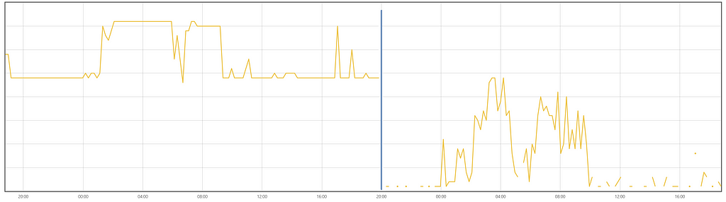
For example, after we adjusted the idle timeout properties, the resource utilization changed as follows:
Image by author
Preventive restart
In our environment, the Spark Connect server (version 3.5) may become unstable after a few days of continuous operation. Most often, we face randomly hanging client application jobs for an infinite amount of time, but there may be other problems as well. Also, over time, the probability of a random failure of the entire Spark Connect server increases dramatically, and this can happen at the wrong moment.
As this component evolves, it will likely become more stable (or we will find out that we have done something wrong in our Spark Connect setup). But currently, the simplest solution has turned out to be a daily preventive restart of the Spark Connect server at a suitable moment (i.e., when no client applications are running on it). An example of what the restart code might look like can be found here.
Conclusion
In this article, I described our experience using Spark Connect to run a large number of diverse Spark applications.
To summarize the above:
This component can help save resources and reduce the wait time for the execution of Spark client applications.
It is better to be careful about which applications should be run on the shared Spark Connect server, as resource-intensive applications may cause problems for the entire system.
You can create an infrastructure for launching client applications so that the decision on how to run any application (either as a separate Spark application or as a Spark Connect client) can be made automatically at the moment of launch.
It is important to note that not all applications will be able to run on Spark Connect, but the number of such cases can be significantly reduced. If there is a possibility of running applications that have not been tested for compatibility with the Spark Connect version of SparkSession API, it is worth implementing a fallback to separate Spark applications.
It is worth paying attention to the Spark properties that can improve resource utilization and increase the overall stability of the Spark Connect server. It may also be reasonable to set up a periodic preventive restart of the Spark Connect server to reduce the probability of accidental failure and unwanted behavior.
Overall, we have had a positive experience using Spark Connect in our company. We will continue to watch the development of this technology with great interest, and there is a plan to expand its use.
Adopting Spark Connect was originally published in Towards Data Science on Medium, where people are continuing the conversation by highlighting and responding to this story.
There are many different algorithms for feature extraction, depending on the type of features it focuses on, such as texture, color, or shape, whether it describes the image as a whole or just local information.
The HOG algorithm is one of the most essential techniques in feature extraction as it is a fundamental step for object detection and recognition tasks.
In this article, we will explore the principles and implementation of the HOG algorithm.
What is a Histogram of Oriented Gradients (HOG)?
The HOG is a global descriptor (feature extraction) method applied to each pixel within an image to extract neighborhood information(neighborhood of pixel) like texture and compress/abstract that information from a given image into a reduced/condensed vector form called a feature vector that could describe the feature of this image which is very useful when it came to captures edge and gradient structures in an image. Moreover, we can compare this processed image for object recognition or object detection.
The HOG Explanation
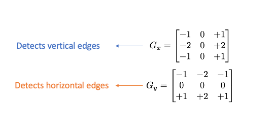
1- Calculate the Gradient Image
To extract and capture edge information, we apply a Sobel operator consisting of two small matrices (filter/kernel) that measure the difference in intensity at grayscale(wherever there is a sharp change in intensity).
created by author
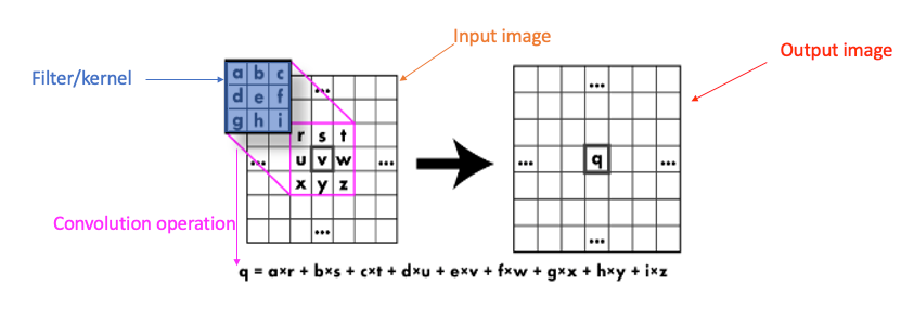
We apply this kernel on pixels of the image by convolution :
We slide the 3×3 Kerne/filter (Sobel Operator) over the image, multiply element-wise, and add the outputs. (Created by the author)
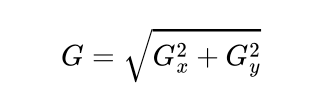
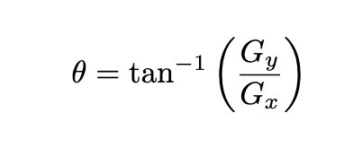
After applying Sobel Kernel to the image now, we can calculate the magnitude and orientation of an image :
Gradient magnitude.(Created by author)Gradient orientation.(Created by author)
The gradients determine the edges’ strength (magnitude) and direction (orientation) at a specific point. The edge direction is perpendicular to the gradient vector’s direction at the location where the gradient is calculated. In other words, the length and direction of the vector.
2- Calculate the Histogram of the Gradient
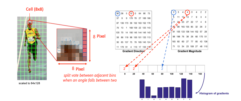
For each pixel, we have two values: magnitude and orientation. To combine this information into something meaningful, we use a histogram, which helps organize and interpret these values effectively.
We create a histogram of gradients in these cells ( 8 x 8 ), which have 64 values distributed to bins in the histogram, which are quantized into 9 bins each of 20 degrees ( spanning 0° to 180°). Each pixel’s magnitude value (edge strength) is added as a “vote” to the corresponding orientation bin so the histogram’s peaks reveal the pixel’s dominant orientations.
3- Normalization
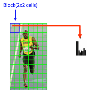
Since gradient magnitudes depend on lighting conditions, normalization scales the histograms to reduce the influence of lighting and contrast variations.
Each block typically consists of a grid of cells (2×2). This block slides across the image with overlap, meaning each cell is included in multiple blocks. Each block has 4 histograms ( 4 cells ), which can be concatenated to form a 4(cells) x 9 (bins )x1 vector = 36 x 1 element vector for each block; overall image in the example: 7 rows x 15 cols = 7x15x36=3780 elements. This feature vector is called the HOG descriptor, and the resulting vector is used as input for classification algorithms like SVM.
# we will be using the hog descriptor from skimage since it has visualization tools available for this example import cv2 import matplotlib.pyplot as plt from skimage import color, feature, exposure
# Load the image img = cv2.imread('The path of the image ..')
# Convert the original image to RGB img_rgb = cv2.cvtColor(img, cv2.COLOR_BGR2RGB)
# Convert the original image to gray scale img_gray = cv2.cvtColor(img_rgb,cv2.COLOR_RGB2GRAY)
plt.imshow(img_gray,cmap="gray")
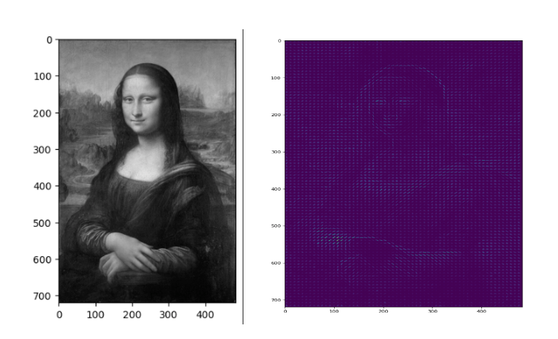
# These are the usual main parameters to tune in the HOG algorithm. (H,Himage) = feature.hog(img_gray, orientations=9, pixels_per_cell=(8,8), cells_per_block=(2,2),visualize=True)
As you can see, HOG effectively captures the general face shape (eyes, nose, head) and hands. This is due to HOG’s focus on gradient information across the image, making it highly effective for detecting lines and shapes. Additionally, we can observe the dominant gradients and their intensity at each point in the image.
(HOG) algorithm for human detection in an image
HOG is a popular feature descriptor in computer vision, particularly effective for detecting shapes and outlines, such as the human form. This code leverages OpenCV’s built-in HOG descriptor and a pre-trained Support Vector Machine (SVM) model specifically trained to detect people
# Load the image
img = cv2.imread('The path of the image ..')

# Convert the original image to RGB
img_rgb = cv2.cvtColor(img, cv2.COLOR_BGR2RGB)

# Convert the original image to gray scale
img_gray = cv2.cvtColor(img_rgb,cv2.COLOR_RGB2GRAY)

#Initialize the HOG descriptor and set the default SVM detector for people
hog = cv2.HOGDescriptor()
hog.setSVMDetector(cv2.HOGDescriptor_getDefaultPeopleDetector())

# Detect people in the image using the HOG descriptor
bbox, weights = hog.detectMultiScale(img_gray ,winStride = (2,2), padding=(10,10),scale=1.02)

# Draw bounding boxes around detected people
for (x, y, w, h) in bbox:
    cv2.rectangle(img_rgb, (x, y),
                  (x + w, y + h),
                  (255, 0, 0), 4)

plt.imshow(img_rgb)
After loading the test image, we use HOG’s detectMultiScale method to detect people, with winStride set to skip one pixel per step, improving speed by trading off a bit of accuracy, which is crucial in object detection since it is a computationally intensive process. Although the detector may identify all people, sometimes there’s a false positive where part of one person’s body is detected as another person. To fix this, we can apply Non-Maxima Suppression (NMS) to eliminate overlapping bounding boxes, though bad configuration(winterize, padding, scale) can occasionally fail to detect objects.
Wrap-up
wrap –up The HOG descriptor computation involves several steps: 1. Gradient Computation 2. Orientation Binning 3. Descriptor Blocks 4. Normalization 5. Feature Vector Formation In this article, we explored the math behind HOG and how easy it is to apply in just a few lines of code, thanks to OpenCV! I hope you found this guide helpful and enjoyed working through the concepts. Thanks for reading, and see you in the next post!
In this post, we share how Hearst, one of the nation’s largest global, diversified information, services, and media companies, overcame these challenges by creating a self-service generative AI conversational assistant for business units seeking guidance from their CCoE.
Building a 28% more accurate multimodal image search engine with VLMs.
Until recently, AI models were narrow in scope and limited to understanding either language or specific images, but rarely both.
In this respect, general language models like GPTs were a HUGE leap since we went from specialized models to general yet much more powerful models.
But even as language models progressed, they remained separate from computer vision аreas, each domain advancing in silos without bridging the gap. Imagine what would happen if you could only listen but not see, or vice versa.
My name is Roman Isachenko, and I’m part of the Computer Vision team at Yandex.
In this article, I’ll discuss visual language models (VLMs), which I believe are the future of compound AI systems.
I’ll explain the basics and training process for developing a multimodal neural network for image search and explore the design principles, challenges, and architecture that make it all possible.
Towards the end, I’ll also show you how we used an AI-powered search product to handle images and text and what changed with the introduction of a VLM.
Let’s begin!
What Are VLMs?
LLMs with billions or even hundreds of billions of parameters are no longer a novelty.
We see them everywhere!
The next key focus in LLM research has been more inclined towards developing multimodal models (omni-models) — models that can understand and process multiple data types.
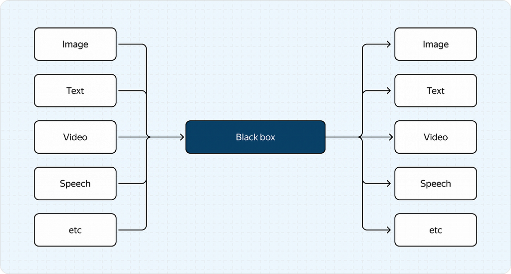
Multimodal models (Image by Author)
As the name suggests, these models can handle more than just text. They can also analyze images, video, and audio.
But why are we doing this?
Jack of all trades, master of none, oftentimes better than master of one.
In recent years, we’ve seen a trend where general approaches dominate narrow ones.
Think about it.
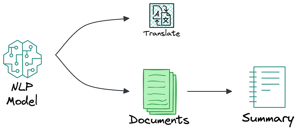
Today’s language-driven ML models have become relatively advanced and general-purpose. One model can translate, summarize, identify speech tags, and much more.
General NLP model (Image by Author)
But earlier, these models used to be task-specific (we have them now as well, but fewer than before).
A dedicated model for translating.
A dedicated model for summarizing, etc.
In other words, today’s NLP models (LLMs, specifically) can serve multiple purposes that previously required developing highly specific solutions.
Second, this approach allows us to exponentially scale the data available for model training, which is crucial given the finite amount of text data. Earlier, however, one would need task-specific data:
A dedicated translation labeled dataset.
A dedicated summarization dataset, etc.
Third, we believe that training a multimodal model can enhance the performance of each data type, just like it does for humans.
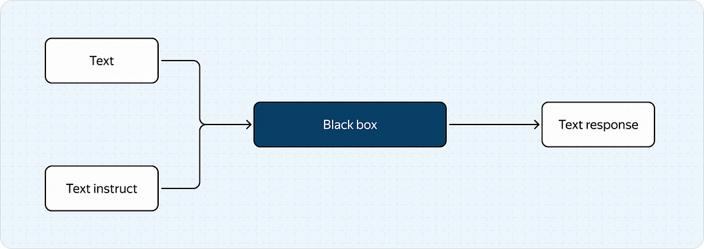
For this article, we’ll simplify the “black box” concept to a scenario where the model receives an image and some text (which we call the “instruct”) as input and outputs only text (the response).
As a result, we end up with a much simpler process as shown below:
A simplified multimodal model (Image by Author)
We’ll discuss image-discriminative models that analyze and interpret what an image depicts.
Before delving into the technical details, consider the problems these models can solve.
A few examples are shown below:
Examples of tasks (Image by Author)
Top left image: We ask the model to describe the image. This is specified with text.
Top mid image: We ask the model to interpret the image.
Top right image: We ask the model to interpret the image and tell us what would happen if we followed the sign.
Bottom image: This is the most complicated example. We give the model some math problems. From these examples, you can see that the range of tasks is vast and diverse.
VLMs are a new frontier in computer vision that can solve various fundamental CV-related tasks (classification, detection, description) in zero-shot and one-shot modes.
While VLMs may not excel in every standard task yet, they are advancing quickly.
Now, let’s understand how they work.
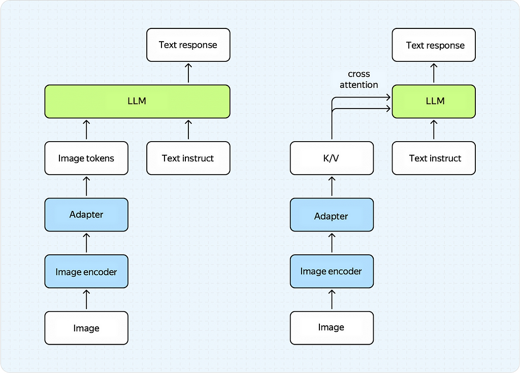
VLM Architecture
These models typically have three main components:
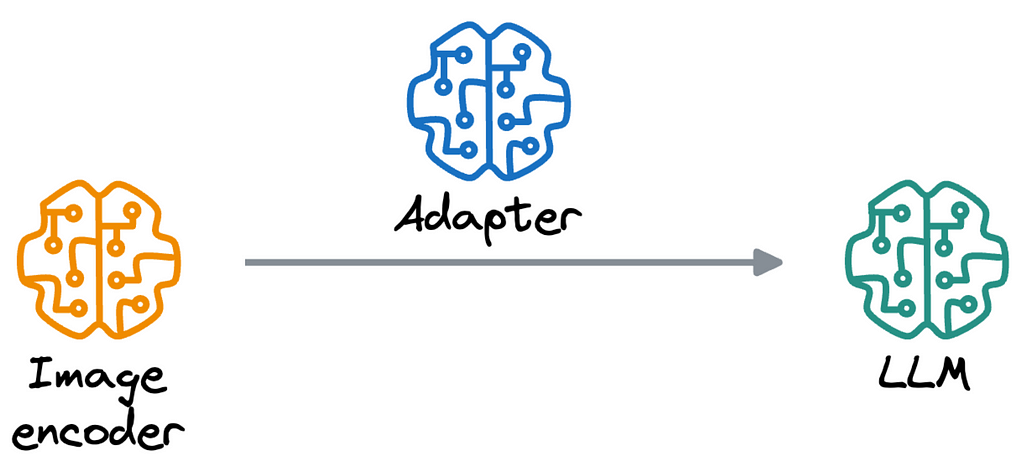
Simplified representation of VLM (Image by Author)
LLM — a text model (YandexGPT, in our case) that doesn’t understand images.
Image encoder — an image model (CNN or Vision Transformer) that doesn’t understand text.
Adapter — a model that acts as a mediator to ensure that the LLM and image encoder get along well.
The pipeline is pretty straightforward:
Feed an image into the image encoder.
Transform the output of the image encoder into some representation using the adapter.
Integrate the adapter’s output into the LLM (more on that below).
While the image is processed, convert the text instruct into a sequence of tokens and feed them into the LLM.
More Information About Adapters
The adapter is the most exciting and important part of the model, as it precisely facilitates the communication/interaction between the LLM and the image encoder.
There are two types of adapters:
Prompt-based adapters
Cross-attention-based adapters
Prompt-based adapters were first proposed in BLIP-2 and LLaVa models.
The idea is simple and intuitive, as evident from the name itself.
We take the output of the image encoder (a vector, a sequence of vectors, or a tensor — depending on the architecture) and transform it into a sequence of vectors (tokens), which we feed into the LLM. You could take a simple MLP model with a couple of layers and use it as an adapter, and the results will likely be pretty good.
Cross-attention-based adapters are a bit more sophisticated in this respect.
They were used in recent papers on Llama 3.2 and NVLM.
These adapters aim to transform the image encoder’s output to be used in the LLM’s cross-attention block as key/value matrices. Examples of such adapters include transformer architectures like perceiver resampler or Q‑former.
Prompt-based adapters (left) and Cross-attention-based adapters (right) (Image by Author)
Prompt-based adapters (left) and Cross-attention-based adapters (right)
Both approaches have pros and cons.
Currently, prompt-based adapters deliver better results but take away a large chunk of the LLM’s input context, which is important since LLMs have limited context length (for now).
Cross-attention-based adapters don’t take away from the LLM’s context but require a large number of parameters to achieve good quality.
VLM Training
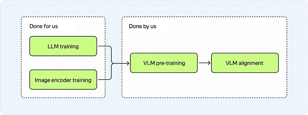
With the architecture sorted out, let’s dive into training.
Firstly, note that VLMs aren’t trained from scratch (although we think it’s only a matter of time) but are built on pre-trained LLMs and image encoders.
Using these pre-trained models, we fine-tune our VLM in multimodal text and image data.
This process involves two steps:
Pre-training
Alignment: SFT + RL (optional)
Training procedure of VLMs (Image by Author)
Notice how these stages resemble LLM training?
This is because the two processes are similar in concept. Let’s take a brief look at these stages.
VLM Pre-training
Here’s what we want to achieve at this stage:
Link the text and image modalities together (remember that our model includes an adapter we haven’t trained before).
Load world knowledge into our model (the images have a lot of specifics, for one, OCR skills).
There are three types of data used in pre-training VLMs:
Interleaved Pre-training: This mirrors the LLM pre-training phase, where we teach the model to perform the next token prediction task by feeding it web documents. With VLM pre-training, we pick web documents with images and train the model to predict text. The key difference here is that a VLM considers both the text and the images on the page. Such data is easy to come by, so this type of pre-training isn’t hard to scale up. However, the data quality isn’t great, and boosting it proves to be a tough job.
Interleaved Pre-training dataset (Image by Author)
Image-Text Pairs Pre-training: We train the model to perform one specific task: captioning images. You need a large corpus of images with relevant descriptions to do that. This approach is more popular because many such corpora are used to train other models (text-to-image generation, image-to-text retrieval).
Image-Text Pairs Pre-training dataset (Image by Author)
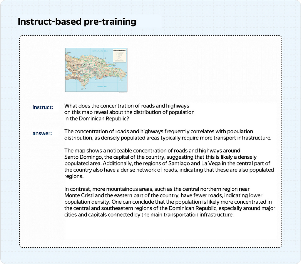
Instruct-Based Pre-training: During inference, we’ll feed the model images and text. Why not train the model this way from the start? This is precisely what instruct-based pre-training does: It trains the model on a massive dataset of image-instruct-answer triplets, even if the data isn’t always perfect.
Instruct-Based Pre-training dataset (Image by Author)
How much data is needed to train a VLM model properly is a complex question. At this stage, the required dataset size can vary from a few million to several billion (thankfully, not a trillion!) samples.
Our team used instruct-based pre-training with a few million samples. However, we believe interleaved pre-training has great potential, and we’re actively working in that direction.
VLM Alignment
Once pre-training is complete, it’s time to start on alignment.
It comprises SFT training and an optional RL stage. Since we only have the SFT stage, I’ll focus on that.
Still, recent papers (like this and this) often include an RL stage on top of VLM, which uses the same methods as for LLMs (DPO and various modifications differing by the first letter in the method name).
Anyway, back to SFT.
Strictly speaking, this stage is similar to instruct-based pre-training.
The distinction lies in our focus on high-quality data with proper response structure, formatting, and strong reasoning capabilities.
This means that the model must be able to understand the image and make inferences about it. Ideally, it should respond equally well to text instructs without images, so we’ll also add high-quality text-only data to the mix.
Ultimately, this stage’s data typically ranges between hundreds of thousands to a few million examples. In our case, the number is somewhere in the six digits.
Quality Evaluation
Let’s discuss the methods for evaluating the quality of VLMs. We use two approaches:
Calculate metrics on open-source benchmarks.
Compare the models using side-by-side (SBS) evaluations, where an assessor compares two model responses and chooses the better one.
The first method allows us to measure surrogate metrics (like accuracy in classification tasks) on specific subsets of data.
However, since most benchmarks are in English, they can’t be used to compare models trained in other languages, like German, French, Russian, etc.
While translation can be used, the errors introduced by translation models make the results unreliable.
The second approach allows for a more in-depth analysis of the model but requires meticulous (and expensive) manual data annotation.
Our model is bilingual and can respond in both English and Russian. Thus, we can use English open-source benchmarks and run side-by-side comparisons.
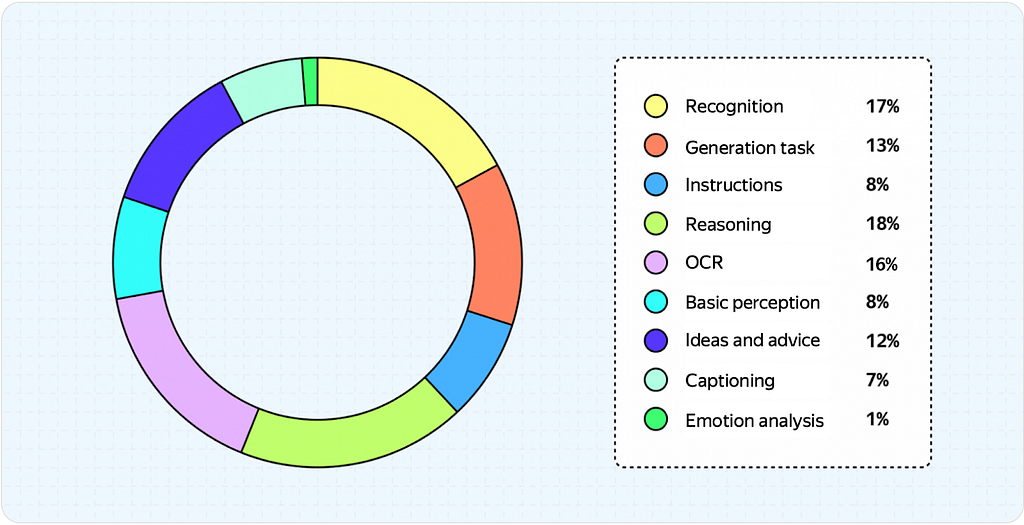
We trust this method and invest a lot in it. Here’s what we ask our assessors to evaluate:
Grammar
Readability
Comprehensiveness
Relevance to the instruct
Errors (logical and factual)
Hallucinations
We strive to evaluate a complete and diverse subset of our model’s skills.
The following pie chart illustrates the distribution of tasks in our SbS evaluation bucket.
Distribution of tasks for quality evaluation (Image by Author)
This summarizes the overview of VLM fundamentals and how one can train a model and evaluate its quality.
Pipeline Architecture
This spring, we added multimodality to Neuro, an AI-powered search product, allowing users to ask questions using text and images.
Until recently, its underlying technology wasn’t truly multimodal.
Here’s what this pipeline looked like before.
Pipeline architecture (Image by Author)
This diagram seems complex, but it’s straightforward once you break it down into steps.
Here’s what the process used to look like
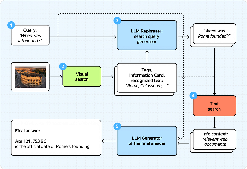
The user submits an image and a text query.
We send the image to our visual search еngine, which would return a wealth of information about the image (tags, recognized text, information card).
We formulate a text query using a rephraser (a fine-tuned LLM) with this information and the original query.
With the rephrased text query, we use Yandex Search to retrieve relevant documents (or excerpts, which we call infocontext).
Finally, with all this information (original query, visual search information, rephrased text query, and info context), we generate the final response using a generator model (another fine-tuned LLM).
Done!
As you can see, we used to rely on two unimodal LLMs and our visual search engine. This solution worked well on a small sample of queries but had limitations.
Below is an example (albeit slightly exaggerated) of how things could go wrong.
The problem with two unimodal LLMs (Image by Author)
Here, the rephraser receives the output of the visual search service and simply doesn’t understand the user’s original intent.
In turn, the LLM model, which knows nothing about the image, generates an incorrect search query, getting tags about the pug and the apple simultaneously.
To improve the quality of our multimodal response and allow users to ask more complex questions, we introduced a VLM into our architecture.
More specifically, we made two major modifications:
We replaced the LLM rephraser with a VLM rephraser. Essentially, we started feeding the original image to the rephraser’s input on top of the text from the visual search engine.
We added a separate VLM captioner to the pipeline. This model provides an image description, which we use as info context for the final generator.
You might wonder
Why not make the generator itself VLM-based?
That’s a good idea!
But there’s a catch.
Our generator training inherits from Neuro’s text model, which is frequently updated.
To update the pipeline faster and more conveniently, it was much easier for us to introduce a separate VLM block.
Plus, this setup works just as well, which is shown below:
Using VLM in AI-powered search (Image by Author)
Training VLM rephraser and VLM captioner are two separate tasks.
For this, we use mentioned earlierse VLM, as mentioned e for thise-tuned it for these specific tasks.
Fine-tuning these models required collecting separate training datasets comprising tens of thousands of samples.
We also had to make significant changes to our infrastructure to make the pipeline computationally efficient.
Gauging the Quality
Now for the grand question:
Did introducing a VLM to a fairly complex pipeline improve things?
In short, yes, it did!
We ran side-by-side tests to measure the new pipeline’s performance and compared our previous LLM framework with the new VLM one.
This evaluation is similar to the one discussed earlier for the core technology. However, in this case, we use a different set of images and queries more aligned with what users might ask.
Below is the approximate distribution of clusters in this bucket.
Cluster distribution (Image by Author)
Our offline side-by-side evaluation shows that we’ve substantially improved the quality of the final response.
The VLM pipeline noticeably increases the response quality and covers more user scenarios.
Accuracy of VLM vs LLM in Neuro (Image by Author)
We also wanted to test the results on a live audience to see if our users would notice the technical changes that we believe would improve the product experience.
So, we conducted an online split test, comparing our LLM pipeline to the new VLM pipeline. The preliminary results show the following change:
The number of instructs that include an image increased by 17%.
The number of sessions (the user entering multiple queries in a row) saw an uptick of 4.5%.
To reiterate what was said above, we firmly believe that VLMs are the future of computer vision models.
VLMs are already capable of solving many out-of-the-box problems. With a bit of fine-tuning, they can absolutely deliver state-of-the-art quality.
Kickstart Your Data Science Journey — A Guide for Aspiring Data Scientists
Key Technical Skills You Need to Kick-start Your Career in Data Science
Are you curious about data science? Does math and artificial intelligence excite you? Do you want to explore data science and plan to pursue a data science career? Whether you’re unsure where to begin or just taking your first steps into data science, you’ve come to the right place. Trust me, this guide will help you take your first steps with confidence!
Data science is one of the most exciting fields in which to work. It’s a multidisciplinary field that combines various techniques and tools to analyze complex datasets, build predictive models, and guide decision-making in businesses, research, and technology.
Data science is applied in various industries such as finance, healthcare, social media, travel, e-commerce, robotics, military, and espionage.
Image generated using GPT 4o
Myths and Truths about Data Science
The Internet has abundant information about how to start with data science, leading to myths and misconceptions about data science. The two most important misconceptions are —
Learn Maths or not?— Many online courses and boot camps advertise that you can become a data scientist in 50 days! These courses are often misleading. They focus on advanced machine learning (ML) topics, a few quick coding tutorials using ML frameworks, and tell you not to get into the nitty-gritty mathematical details. It’s not okay not to worry about the mathematics behind it. Maths is important. Importing libraries, treating models like a black box, and relying on high-level APIs isn’t really data science, especially in product-based companies.
Is Data Science equal to Large Language Models/Generative AI?— No. Data science is not synonymous with large language models (LLMs)/Generative AI. Data science spans far beyond LLMs and encompasses a variety of tools and algorithms. LLMs are groundbreaking but are not suited for solving every academic, research, or business problem. LLMs are one tool among many and shouldn’t define an entire skill set.
Data scientists require a strong grasp of mathematics. It’s important for someone starting their data science journey to focus on mathematics and fundamentals before diving into fancy stuff like LLMs. I’ve stressed the importance of fundamentals throughout this article. The knowledge of basic concepts will help you stand out from the crowd of data science aspirants. It will help you ace this career and stay updated with the developments in this rapidly growing field. Think of it as laying a building’s foundation. It takes the maximum time and effort. It’s essential to support everything that follows. Once the base is solid, you can start building upwards, floor by floor, expanding your knowledge and skills.
What is expected from you?
Patience — Becoming a data scientist is a long, challenging, and tedious journey. Patience is key. Be ready to deal with a few struggles.
Passion — Passion drives success. Your curiosity and enthusiasm for data and problem-solving will fuel your progress.
Growth Mindset — Data science is a vast and rapidly evolving field. Embrace the mindset of continuous learning. Always seek to improve and stay updated.
Think from first principles — Thinking from first principles is the thumb rule in any profession. It helps you solve problems by breaking them down to the basics and building solutions from the base.
Consistency — Consistent efforts compound into grand success. Take small steps constantly.
Knowing where to start might seem overwhelming if you’re a beginner. With so many tools, concepts, and techniques to learn, it’s easy to feel lost. But don’t worry!
In this article —
I will explore the role of a data scientist within an organization and highlight their key responsibilities and contributions.
I’ll discuss the most fundamental technical skills you need to kick-start your career in data science.
I’ll explain why these skills are important.
I’ll share valuable resources to help you learn and develop these skills.
Let’s get started!
Job Description of a Data Scientist
Define the Problem Statement — A data scientist’s role starts by identifying and solving business challenges using data-driven methods and predictive modeling. The first step involves collaborating with product managers and subject matter experts to define a clear and precise problem statement.
Exploratory Data Analysis and Training Models — Data scientists perform data analysis to identify the underlying issues. Once the problem is defined, the next step is to gather and explore the appropriate data required to train an ML model. This is where they apply their primary data science skills and judgment to obtain a robust model.
Model Evaluation — Data scientists play a crucial role in developing and tracking evaluation metrics to quantify the success of ML models. For instance, in an e-commerce recommendation system, these metrics could measure the model’s impact on sales, user engagement, or revenue growth. Defining the right metrics ensures that the model aligns with business objectives and can deliver meaningful value to the business.
Model Deployment and A/B Testing — Once the model is ready, you work closely with engineers to deploy it into production. They conduct A/B testing to validate the model’s effectiveness and scale the model for larger use. They monitor its performance over time.
Research and Experiment— Data scientists continuously experiment with innovative ideas to improve their models. Staying up to date with the latest research is essential. Reading research papers provides insights into new methodologies, algorithms, and breakthroughs.
The following technical skills are necessary.
Mathematics — Linear Algebra, Probability, Statistics, and Calculus
Machine Learning Fundamentals
Coding — Python and SQL
1. Mathematics
Mathematics is everywhere. No doubt it’s the backbone and the core of data science. A good data scientist must have a deep and concise understanding of mathematics. Mastering mathematics will help you
Correctly explore, analyze, and interpret large noisy industrial datasets.
Extract meaningful conclusions from data.
Grasp the foundational principle behind any ML model you want to use.
Tweak the model (model hyperparameters, neural network architecture, loss function) based on your requirements.
Choose the appropriate ML and business metrics to evaluate the models you built.
Generate a feedback loop to detect possible scenarios where the model might fail.
Perform error/root cause analysis to understand model flaws.
Without mathematical understanding, you’ll have difficulty unboxing the black box. The following topics are super important.
1.1. Linear Algebra
Linear Algebra is a beautiful and elegant branch of mathematics that deals with vectors, matrices, and linear transformations. Linear Algebra concepts are fundamental for solving systems of linear equations and manipulating high-dimensional data.
Why is it required?
In industry, data at scale is inherently high-dimensional. Linear algebra provides the mathematical foundation to represent, store, and efficiently manipulate this data using vectors and matrices. Data transformations, projections, and optimizations can be performed easily by leveraging linear algebra concepts like linear transformations, determinants, orthogonality, and rank.
For instance, dimensionality reduction techniques like principal component analysis (PCA) rely on concepts like singular value decomposition to extract meaningful, lower-dimensional representations of large datasets.
Linear algebra is deeply embedded in the core of many ML algorithms. Neural networks and LLMs depend on efficient matrix operations, like matrix multiplications, to handle the massive computational demands of training and inference.
Nvidia folks are getting richer daily because they produce and sell the hardware (GPUs) and write open-source optimized software (Cuda) to perform efficient matrix operations!
Where to learn Linear Algebra?
Professor Gilbert Strang’s MIT lectures — Here. He’s one of the best Linear algebra teachers in the world. Professor Strang is a legend. His explanations and way of teaching make the subject even more interesting.
Sheldon Axler’s Book — Here. You can use Sheldon Axler’s book as a reference book and practice exercises.
3Blue1Brown YouTube Channel — Here. Follow this YouTube channel for eye-catching visualizations of different concepts in Linear algebra.
1.2. Probability and Statistics
Probability and statistics are essential for understanding uncertainty in data-driven fields. Probability theory provides a mathematical framework to quantify the likelihood of events. Statistics involves collecting, organizing, analyzing, and interpreting data to make informed decisions.
Why are they required?
Before diving into ML models, it’s crucial to analyze and understand the basic properties of data. High school concepts like mean, median, mode, variance, quantiles, and standard deviation are foundational for exploring data distributions and trends.
Statistical concepts such as variance, covariance, and correlation are key for identifying relationships between features.
Probability is the core principle that drives predictive modeling. An in-depth understanding of probability axioms, probability density functions, probability distribution functions, random variables (continuous and discrete), Bayes theorem, expectation, variance, joint distributions, and conditional probability is essential.
ML algorithms often assume that the input data and output follow a certain probability distribution. Familiarity with distributions like Gaussian (Normal), Geometric, Bernoulli, Binomial, Poisson, and Beta enables better assumptions about data and models.
In product data science, A/B testing is a common practice to compare variations and make decisions. Knowledge about hypothesis testing using statistical tests like z-test and chi-squared test is useful.
Where to learn Probability and Statistics?
Professor John Tsitsiklis’s MIT Introduction to Probability lectures — Here.
Stanford University’s Probability for Computer Scientists lectures — Here
Josh Starmer’s YouTube Playlist for Statistics— Here. His videos are very engaging. You can follow his YouTube channel to learn other data science concepts. This channel is useful, especially for learning/revising statistics concepts.
Sheldon Ross’s Book — Here. You can use Sheldon Ross’ book as a reference book. Practice exercises from this book.
1.3. Calculus
Calculus is about finding the rate of change of a function. Calculus, especially differential calculus, plays an integral role in ML. It calculates the slope or gradient of curves, which tells us how a quantity changes in response to changes in another.
Why is it required?
The ML algorithm aims to obtain a set of parameters with the least prediction error (or loss function). Optimization algorithms like gradient descent are used extensively to minimize the prediction error and update the model parameters.
In deep learning, the chain rule of differentiation is critical for the backpropagation algorithm. Backpropagation computes gradients efficiently through deep neural networks. It’s fundamental to understanding how neural networks work and how gradients are used to obtain the best model parameters.
The 2024 Nobel Laureate Geoffrey Hinton co-authored the backpropagation algorithm paper in 1986!
Where to learn Calculus?
Wait! You’ll find it out soon!
2. Machine Learning Fundamentals
Machine learning is built upon the core principles of Linear algebra, probability, statistics, and calculus. At its essence, ML is applied mathematics, and once you grasp the underlying mathematics, understanding fundamental ML concepts becomes much easier. These fundamentals are essential for building robust and accurate ML models.
Most comprehensive ML courses begin by introducing the various types of algorithms. There are supervised, unsupervised, self-supervised, and reinforcement learning methods, each designed for specific problems. ML algorithms are further categorized into classification, regression, and clustering, depending on whether the task predicts labels, continuous values, or identifies patterns.
Nearly all ML workflows follow a structured process, which includes the following key steps:
Feature Engineering and Data Preprocessing — Although it might not be the most glamorous part of data science, feature engineering and data preprocessing play a pivotal role in determining how well your machine learning models will perform. This involves splitting your data into train, validation, and test sets. Other key activities include dimensionality reduction, feature selection, normalization, and handling outliers. Properly addressing missing values and class imbalance (in classification tasks) is crucial to prevent biased or inaccurate models. These steps ensure your data is clean and properly structured, allowing the model to focus on learning from meaningful patterns rather than noise.
Image AI-generated by GPT 4o
Training and Optimization — Probability and statistics play a pivotal role in defining the loss function of an ML algorithm. A key concept, maximum likelihood estimation (MLE), is often used to derive the loss function based on our assumptions about the data’s distribution. During training, the model’s parameters (weights) are updated iteratively by optimizing the loss function. As you might have guessed, this is done using gradient descent algorithms. Mathematics everywhere!
Overfitting and Underfitting — These are two of the many challenges we face while training ML models. Overfitting occurs when a model learns noise in the training data and performs poorly on unseen data. Underfitting happens when a model is too simple to capture the underlying patterns, leading to poor training and test data performance. Bias-variance tradeoffis the balance between model complexity and generalization. High bias leads to underfitting, and high variance leads to overfitting. The ability to manage this tradeoff by varying hyperparameters, applying regularization, and observing validation set performance is one of the important skills of a data scientist.
Evaluation Metrics — As a data scientist, it’s crucial to pick the most suitable metric to evaluate your model. Evaluation is done on the test set. There are a plethora of ML metrics suitable to different problem scenarios.
Where to learn ML?
Andrew Ng’s Stanford University’s ML Specialization — Here. I undertook this course in 2019. It remains the best course for understanding basic ML. You can audit this course for free! This specialization doesn’t cover the math deeply but gives you an intuitive understanding of ML.
Cornell Tech’s Applied Machine Learning Lectures — Here. This course is super important. It starts with a primer on calculus and optimization before diving deep into the nitty-gritty details of various ML algorithms. You’ll witness the amalgamation of linear algebra, probability, and calculus concepts here. Lecture notes are available in the link shared above.
These courses will cover ML algorithms such as linear regression, Bayes classifier, logistic regression, k-means clustering, Gaussian mixture models, support vector machines, neural networks, decision trees, random forests, and boosting algorithms.
A clear understanding of mathematics and ML fundamentals opens the avenues for exploring advanced concepts like deep learning, natural language processing, computer vision, recommendation systems, generative AI, and large language models (LLMs).
You might have noticed a pattern. I have provided you with resources involving lectures from top universities like MIT, Stanford University, Carnegie Mellon University, and Cornell Tech. From next time onwards, look for course lectures from these universities whenever you want to upskill. They offer the best explanation and content. For instance, Stanford University has courses on Deep Learning for NLP, Graph ML, and Reinforcement Learning on its YouTube channel.
3. Coding
Coding skills are just as essential as mathematics for thriving as a data scientist. Coding skills help develop your problem-solving and critical-thinking abilities. Python and SQL are the most important coding skills you must possess.
3.1 Python
Python is the most widely used programming language in data science due to its simplicity, versatility, and powerful libraries.
What will you have to do?
Your first target must be learning basic data structures like strings, lists/arrays, dictionaries, and core Object-Oriented Programming (OOP) concepts like classes and objects. Become an expert in these two areas.
Knowledge of advanced data structures like trees, graphs, and traversal algorithms is a plus point.
You must be proficient in time and space complexity analysis. It’ll help you write efficient code in practice. Learning the basic sorting and searching algorithms can help you gain a sufficient understanding of time and space complexity.
Python has the best data science library collection. Two of the most essential libraries are —
NumPy — This library supports efficient operations on vectors and matrices.
Pandas/PySpark — Pandas is a powerful data frame library for data manipulation and analysis. It can handle structured data formats like .csv, .parquet, and .xlsx. Pandas dataframes support operations that simplify tasks like filtering, sorting, and aggregating data. Pandas library is good for handling small datasets. The PySpark library is used to handle big data. It supports a variety of SQL operations (discussed later in the article), making it ideal for working with large datasets in distributed environments.
Beyond these, there are several other libraries you’ll encounter and use regularly —
Scikit-learn — A go-to library for implementing machine learning algorithms, data preprocessing, and model evaluation.
PyTorch — A deep learning framework widely used for building and training neural networks.
Matplotlib and Seaborn — Libraries for data visualization, allowing you to create plots, charts, and graphs to visualize and understand data.
As a beginner, mastering every library isn’t a requirement. There are countless domain-specific libraries, like OpenCV, statsmodel, and Transformers, that you’ll pick up naturally through hands-on practice. Learning to use libraries is one of the easiest parts of data science and becomes second nature as you work on more projects. There’s no need to memorize functions — honestly, I still google various Pandas and PySpark functions all the time! I’ve seen many aspirants focus solely on libraries. While libraries are important, they’re just a small part of your toolkit.
3.2 SQL
SQL (Structured query language) is a fundamental tool for data scientists, especially when working with large datasets stored in relational databases. Data in many industries is stored in relational databases like SQL. SQL is one of the most important skills to hone when starting your data science journey. SQL allows you to query, manipulate, and retrieve data efficiently. This is often the first step in any data science workflow. Whether you’re extracting data for exploratory analysis, joining multiple tables, or performing aggregate operations like counting, averaging, and filtering, SQL is the go-to language.
I had only a basic understanding of SQL queries when I started my career. That changed when I joined my current company, where I began using SQL professionally. I worked with industry-level big data, ran SQL queries to fetch data, and gained hands-on experience.
The following SQL statements and operations are important —
Basic —
Extraction —The select statement is the most basic statement in SQL querying.
Filtering —The where keyword is used to filter data as per conditions.
Sorting — The order by keyword is used to order the data in either asc or desc order.
Joins — As the name suggests, SQL Joins help you join multiple tables in your SQL database. SQL has different types of joins — left, right, inner, outer, etc.
Aggregation Functions— SQL supports various aggregation functions such as count(), avg(), sum(), min(), max().
Grouping — The group by keyword is often used with an aggregation function.
Advanced —
Window Functions — Window functions are a powerful feature in SQL that allows you to perform calculations across a set of table rows related to the current row. Once you are proficient with the basic SQL queries mentioned above, familiarize yourself with window functions such as row_number(), rank(), dense_rank(), lead(), lag(). Aggregation functions can also be used as window functions. The partition by keyword is used to partition the set of rows (called the window) and then perform the window operations.
Common Table Expressions (CTEs) — CTEs make SQL queries more readable and modular, especially when working with complex subqueries or recursive queries. They are defined using the with keyword. This is an advanced concept.
You’ll often use Python’s PySpark library in conjunction with SQL. PySpark has APIs for all SQL operations and helps integrate SQL and Python. You can perform various SQL operations on PySpark dataframes in Python seamlessly!
3.3 Practice, Practice, Practice
Rigorous practice is key to mastering coding skills, and platforms like LeetCode and GeeksForGeeks offer great tutorials and exercises to improve your Python skills.
SQLZOO and w3schools are great platforms to start learning SQL.
Kaggle is the best place to combine your ML and coding skills to solve ML problems. It’s important to get hands-on experience. Pick up any contest. Play with the dataset and apply the skills you learn from the lectures.
Implementing ML algorithms without using special ML libraries like scikit-learn or PyTorch is a great self-learning exercise. Writing code from scratch for basic algorithms like PCA, gradient descent, and linear/logistic regression can help you enhance your understanding and coding skills.
During my Master’s in AI course at the Indian Institute of Science, Bengaluru, we had coding assignments where we implemented algorithms in C! Yes C! One of these assignments was about training a deep neural network for MNIST digits classification.
I built a deep neural network from scratch in C. I created a custom data structure for storing weights and wrote algorithms for gradient descent and backpropagation. I felt immense satisfaction when the C code ran successfully on my laptop’s CPU. My friend mocked me for doing this “impractical” exercise and argued that we have highly efficient libraries for such a task. Although my code was inefficient, writing the code from scratch deepened my understanding of the internal mechanics of deep neural networks.
You’ll eventually use libraries for your projects in academia and industry. However, as a beginner, jumping straight into libraries can prevent you from fully understanding the fundamentals.
Congratulations on making it this far in the article! We’ve covered the core skills necessary to become a data scientist. By now, I hope you have a solid understanding of why the basics are so important.
A Master’s degree from a reputed institution can provide structured learning on mathematics and ML concepts. It also offers opportunities to work on projects and gain practical experience. However, if pursuing a formal degree isn’t an option, don’t worry. You can follow the YouTube playlists and reference books mentioned earlier to self-learn.
Every expert was once a beginner. The key is to start small. Take it one step at a time, and gradually build your knowledge. Make sure not to skip any steps — start by mastering the math before moving on to applying it. Don’t rush the process. Focus on truly understanding each concept. Developing a strong foundation and thinking from first principles should always be your mantra. Over time, everything will begin to fall into place. With the right mindset, you’ll excel in this journey.
I highly recommend becoming a Medium member if you haven’t done so. You’ll unlock unlimited access to invaluable resources. Trust me, it’s a goldmine of knowledge! You’ll find insightful articles written by data science professionals and experts.
I hope you find my article interesting. Thank you for reading, and good luck in your data science journey!
We use cookies on our website to give you the most relevant experience by remembering your preferences and repeat visits. By clicking “Accept”, you consent to the use of ALL the cookies.
This website uses cookies to improve your experience while you navigate through the website. Out of these, the cookies that are categorized as necessary are stored on your browser as they are essential for the working of basic functionalities of the website. We also use third-party cookies that help us analyze and understand how you use this website. These cookies will be stored in your browser only with your consent. You also have the option to opt-out of these cookies. But opting out of some of these cookies may affect your browsing experience.
Necessary cookies are absolutely essential for the website to function properly. These cookies ensure basic functionalities and security features of the website, anonymously.
Cookie
Duration
Description
cookielawinfo-checkbox-analytics
11 months
This cookie is set by GDPR Cookie Consent plugin. The cookie is used to store the user consent for the cookies in the category "Analytics".
cookielawinfo-checkbox-functional
11 months
The cookie is set by GDPR cookie consent to record the user consent for the cookies in the category "Functional".
cookielawinfo-checkbox-necessary
11 months
This cookie is set by GDPR Cookie Consent plugin. The cookies is used to store the user consent for the cookies in the category "Necessary".
cookielawinfo-checkbox-others
11 months
This cookie is set by GDPR Cookie Consent plugin. The cookie is used to store the user consent for the cookies in the category "Other.
cookielawinfo-checkbox-performance
11 months
This cookie is set by GDPR Cookie Consent plugin. The cookie is used to store the user consent for the cookies in the category "Performance".
viewed_cookie_policy
11 months
The cookie is set by the GDPR Cookie Consent plugin and is used to store whether or not user has consented to the use of cookies. It does not store any personal data.
Functional cookies help to perform certain functionalities like sharing the content of the website on social media platforms, collect feedbacks, and other third-party features.
Performance cookies are used to understand and analyze the key performance indexes of the website which helps in delivering a better user experience for the visitors.
Analytical cookies are used to understand how visitors interact with the website. These cookies help provide information on metrics the number of visitors, bounce rate, traffic source, etc.
Advertisement cookies are used to provide visitors with relevant ads and marketing campaigns. These cookies track visitors across websites and collect information to provide customized ads.