Tag: AI

The interplay between ownership, outsourcing, and remote work

As we enter 2025, artificial intelligence (AI) is taking center stage at companies across industries. Faced with the twin challenges of acting decisively in the short run (or at least appearing to do so to reassure various stakeholders) and securing a prosperous future for the company in the long run, executives may be compelled to launch strategic AI initiatives. The aims of these initiatives can range from upgrading the company’s technical infrastructure and harvesting large amounts of high-quality training data, to improving the productivity of employees and embedding AI across the company’s products and services to offer greater value to customers.

Organizing in the right way is crucial to the successful implementation of such AI initiatives and can depend on a company’s particular context, e.g., budgetary constraints, skills of existing employees, and path dependency due to previous activities. This article takes a closer look at the interplay between three key dimensions of organizing for AI in today’s complex world: ownership, outsourcing, and proximity. We will see how different combinations of these dimensions could manifest themselves in the AI initiatives of various companies, compare pros and cons, and close with a discussion of past, present, and future trends.

Note: All figures and tables in the following sections have been created by the author of this article.

Guiding Framework

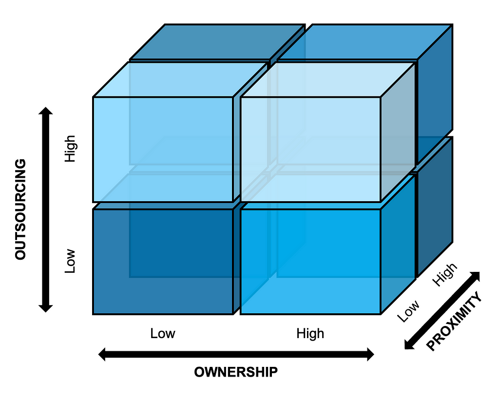
Figure 1 below visualizes the interplay between the three dimensions of ownership, outsourcing, and proximity, and this will serve as the guiding framework for the rest of the article.

The ownership dimension reflects whether the team implementing a given initiative will also own the initiative going forward, or instead act as consultants to another team that will take over long-term ownership. The outsourcing dimension captures whether the team for the initiative is primarily staffed with the company’s own employees or external consultants. Lastly, the proximity dimension considers the extent to which team members are co-located or based remotely; this dimension has gained in relevance following the wide experimentation with remote work by many companies during the global COVID-19 pandemic and throughout the escalation of geopolitical tensions around the world since then.

Although Figure 1 depicts the dimensions as clear-cut dichotomies for the sake of simplicity (e.g., internal versus external staffing), they of course have shades of gray in practice (e.g., hybrid approaches to staffing, industry partnerships). In their simplified form, the boxes in Figure 1 suggest eight possible ways of organizing for AI initiatives in general; we can think of these as high-level organizational archetypes. For example, to build a flagship AI product, a company could opt for an internally staffed, co-located team that takes full long-term ownership of the product. Alternatively, the company might choose to set up an outsourced, globally dispersed team, to benefit from a broader pool of AI talent.

Organizational Archetypes for AI

Table 1 below provides an overview of the eight high-level organizational archetypes, including real-life examples from companies around the world. Each archetype has some fundamental pros and cons that are largely driven by the interplay between the constituent dimensions.

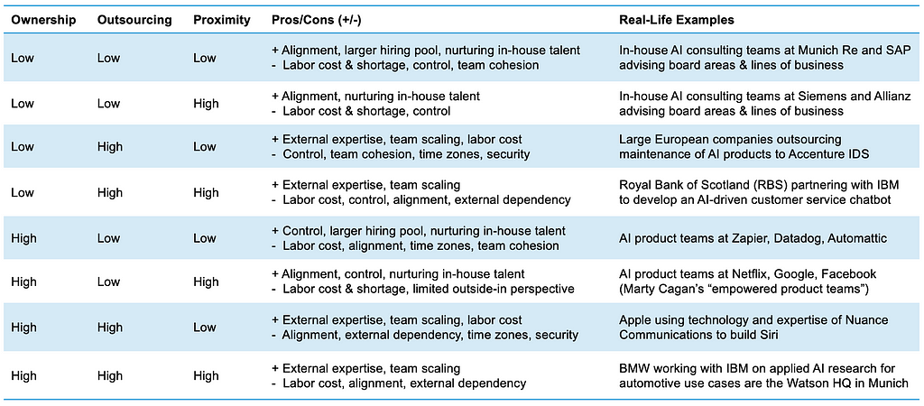
Archetypes with high ownership tend to offer greater long-term accountability, control, and influence over the outcomes of the AI initiative when the level of outsourcing is minimal, since in-house team members typically have more “skin in the game” than external consultants. But staffing AI experts internally can be expensive, and CFOs may be especially wary of this given the uncertain return on investment (ROI) of many early AI initiatives. It may also be harder to flexibly allocate and scale the scarce supply of in-house experts across different initiatives.

Meanwhile, archetypes that combine a high level of outsourcing and low proximity can allow AI initiatives to be implemented more cost-effectively, flexibly, and with greater infusion of specialized external expertise (e.g., a US-based company building an AI product with the help of externally sourced AI experts residing in India), but they come with cons such as external dependencies that can result in vendor lock-in and lower retention of in-house expertise, security risks leading to reduced protection of intellectual property, and difficulties in collaborating effectively with geographically dispersed external partners, potentially across time zones that are inconveniently far apart.

Current and Future Trends

As the real-life examples listed in Table 1 show, companies are already trying out different organizational archetypes. Given the trade-offs inherent to each archetype, and the nascent state of AI adoption across industries overall, the jury is still out on which archetypes (if any) lead to more successful AI initiatives in terms of ROI, positive market signaling, and the development of a sustained competitive advantage.

However, some archetypes do seem to be more common today — or at least have more vocal evangelists — than others. The combination of high ownership, low outsourcing, and high proximity (e.g., core AI products developed by co-located in-house teams) has been the preferred archetype of successful tech companies like Google, Facebook, and Netflix, and influential product coaches such as Marty Cagan have done much to drive its adoption globally. Smaller AI-first companies and startups may also opt for this organizational archetype to maximize control and alignment across their core AI products and services. But all these companies, whether large or small, tend to show strong conviction about the value that AI can create for their businesses, and are thus more willing to commit to an archetype that can require more funding and team discipline to execute properly than others.

For companies that are earlier in their AI journeys, archetypes involving lower ownership of outcomes, and greater freedom of outsourcing and remote staffing tend to be more attractive today; this may in part be due to a combination of positive signaling and cautious resource allocation that such archetypes afford. Although early-stage companies may not have identified a killer play for AI yet, they nonetheless want to signal to stakeholders (customers, shareholders, Wall Street analysts, and employees) that they are alert to the strategic significance of AI for their businesses, and ready to strike should a suitable opportunity present itself. At the same time, given the lack of a killer play and the inherent difficulty of estimating the ROI of early AI initiatives, these companies may be less willing to place large sticky bets involving the ramp-up of in-house AI staff.

Looking to the future, a range of economic, geopolitical, and technological factors will likely shape the options that companies may consider when organizing for AI. On the economic front, the cost-benefit analysis of relying on external staffing and taking ownership of AI initiatives may change. With rising wages in countries such as India, and the price premium attached to high-end AI services and expertise, the cost of outsourcing may become too high to justify any benefits. Moreover, for companies like Microsoft that prioritize the ramp-up of internal AI R&D teams in countries like India, it may be possible to reap the advantages of internal staffing (alignment, cohesion, etc.) while benefiting from access of affordable talent. Additionally, for companies that cede ownership of complex, strategic AI initiatives to external partners, switching from one partner to another may become prohibitively expensive, leading to long-term lock-in (e.g., using the AI platform of an external consultancy to develop custom workflows and large-scale models that are difficult to migrate to more competitive providers later).

The geopolitical outlook, with escalating tensions and polarization in parts of Eastern Europe, Asia, and the Middle East, does not look reassuring. Outsourcing AI initiatives to experts in these regions can pose a major risk to business continuity. The risk of cyber attacks and intellectual property theft inherent to such conflict regions will also concern companies seeking to build a lasting competitive advantage through AI-related proprietary research and patents. Furthermore, the threat posed by polarized national politics in mature and stagnating Western economies, coupled with the painful lessons learned from disruptions to global supply chains during the COVID-19 pandemic, might lead states to offer greater incentives to reshore staffing for strategic AI initiatives.

Lastly, technologies that enable companies to organize for AI, and technologies that AI initiatives promise to create, will both likely inform the choice of organizational archetypes in the future. On the one hand, enabling technologies related to online video-conferencing, messaging, and other forms of digital collaboration have greatly improved the remote working experience of tech workers. On the other hand, in contrast to other digital initiatives, AI initiatives must navigate complex ethical and regulatory landscapes, addressing issues around algorithmic and data-related bias, model transparency, and accountability. Weighing the pros and cons, a number of companies in the broader AI ecosystem, such as Zapier and Datadog, have adopted a remote-first working model. The maturity of enabling technologies (increasingly embedded with AI), coupled with the growing recognition of societal, environmental, and economic benefits of fostering some level of remote work (e.g., stimulating economic growth outside big cities, reducing pollution and commute costs, and offering access to a broader talent pool), may lead to further adoption and normalization of remote work, and spur the development of best practices that minimize the risks while amplifying the advantages of low proximity organizational archetypes.

---

Organizing for AI was originally published in Towards Data Science on Medium, where people are continuing the conversation by highlighting and responding to this story.

You can’t afford to remain an AI-ignoramus, even if your product isn’t using an LLM

If you’re a Software Architect, or a Tech Lead, or really anyone senior in tech whose role includes making technical and strategic decisions, and you’re not a Data Scientist or Machine Learning expert, then the likelihood is that Generative AI and Large Language Models (LLMs) were new to you back in 2023.

AI was certainly new to me.

We all faced a fork in the road —should we invest the time and effort to learn GenAI or continue on our jolly way?

At first, since the products I’m working on are not currently using AI, I dipped my toes in the water with some high-level introductory training on AI, and then went back to my day job of leading the architecture for programmatic features and products. I reassured myself that we can’t all be experts in everything — the same way I’m not a computer vision expert, I don’t need to be an AI expert — and instead I should remain focused on high level architecture along with my core areas of expertise- cloud and security.

Did you face a similar decision recently?

I’m guessing you did.

I’m here to tell you that if you chose the path of LLM-semi-ignorance, you’re making a huge mistake.

Luckily for me, I was part of a team that won a global hackathon for our idea around using AI for improving organizational inclusivity, and that kicked off a POC using GenAI. That then led to co-authoring a patent centered around LLM fine-tuning. I was bothered by my ignorance when AI terms flew around me, and started investing more in my own AI ramp-up, including learning from the experts within my organization, and online courses which went beyond the introductory level and into the architecture. Finally it all clicked into place. I’m still not a data scientist, but I can understand and put together a GenAI based architecture. This enabled me to author more patents around GenAI, lead an experimental POC using an LLM and AI agents, and participate in a GenAI hackathon.

What I learned from this experience is that GenAI is introducing entirely new paradigms, which are diametrically opposed to everything I knew until now. Almost every single fact from my computer science degrees, academic research, and work experience is turned on its head when I’m designing a GenAI system.

GenAI means solving problems using non-deterministic solutions. We got used to programmatic and deterministic algorithms, allowing us to predict and validate inputs against outputs. That’s gone. Expect different results each time, start thinking about a percentage of success vs absolute correctness.

GenAI means results are not linear to development effort investment. Some problems are easy to solve with a simple prompt, others require prior data exploration and complex chains of multiple agentic AI workflows, and others require resource heavy fine tuning. This is very different than assessing a requirement, translating it to logical components and being able to provide an initial decomposition and effort assessment. When we use an LLM, in most cases, we have to get our hands dirty and try it out before we can define the software design.

As a software architect, I’ve begun assessing tradeoffs around using GenAI vs sticking with class programmatic approaches, and then digging deeper to analyze tradeoffs within GenAI — Should we using fine tuning vs. RAG, where is an AI agent needed? Where is further abstraction and multi-agents needed? Where should we combine programmatic pre-processing with an LLM?

For every single one of these architectural decision points- GenAI understanding is a must.

I became a Software Architect after over a decade of experience as a Software Engineer, developing code in multiple languages and on multiple tech stacks, from embedded to mobile to SaaS. I understand the nuts and bolts of programmatic code, and even though I’m not writing code anymore myself, I rely on my software development background both for making high level decisions and for delving into the details when necessary. If as tech leaders we don’t ensure that we gain equivalent knowledge and hands-on experience in the field of GenAI, we won’t be able to lead the architecture of modern systems.

In other words — I realized that I cannot be a good Software Architect, without knowing GenAI. The same way I can’t be a good Software Architect if I don’t understand topics such as algorithms, complexity, scaling; architectures such as client-server, SaaS, relational and non-relational data bases; and other computer science foundations.

GenAI has become foundational to computer engineering. GenAI is no longer a niche sub-domain that can be abstracted away and left to Subject Matter Experts. GenAI means new paradigms and new ways of thinking about software architecture and design. And I don’t think any Software Architect or Tech Leader can reliably make decisions without having this knowledge.

It could be that the products and projects you lead will remain AI free. GenAI is not a silver bullet, and we need to ensure we don’t replace straightforward automation with AI when it’s not needed and even detrimental. All the same, we need to be able to at least assess this decision knowledgeably, every time we face it.

I’m going to end with some positive news for Software Architects — yes we all have to ramp-up and learn AI — but once we do, we’re needed!

As GenAI based tools become ever more complex, data science and AI expertise is not going to be enough — we need to architect and design these systems taking into account all those other factors we’ve been focused on until now — scale, performance, maintainability, good design and composability — there’s a lot that we can contribute.

But first we need to ensure we learn the new paradigms as GenAI transforms computer engineering — and make sure we’re equipped to continue to be technical decision makers in this new world.

---

Why Every Software Architect Needs to Learn GenAI was originally published in Towards Data Science on Medium, where people are continuing the conversation by highlighting and responding to this story.

A discussion around measuring error rates in IBM quantum processors, with code examples, using Qiskit

Quantum computing has made significant strides in recent years, with breakthroughs in hardware stability, error mitigation, and algorithm development bringing us closer to solving problems that classical computers cannot tackle efficiently. Companies and research institutions worldwide are pushing the boundaries of what quantum systems can achieve, transforming this once-theoretical field into a rapidly evolving technology. IBM has emerged as a key player in this space, offering IBM Quantum, a platform that provides access to state-of-the-art quantum processors (QPUs) with a qubit capacity in the hundreds. Through the open-source Qiskit SDK, developers, researchers, and enthusiasts can design, simulate, and execute quantum circuits on real quantum hardware. This accessibility has accelerated innovation while also highlighting key challenges, such as managing the error rates that still limit the performance of today’s quantum devices.

By leveraging the access to quantum processors available for free on the IBM platform, we propose to run a few quantum computations to measure the current level of quantum noise in basic circuits. Achieving a low enough level of quantum noise is the most important challenge in making quantum computing useful. Unfortunately, there is not a ton of material on the web explaining the current achievements. It is also not obvious what quantity we want to measure and how to measure it in practice.

In this blogpost,

• We will review some basics of quantum circuits manipulations in Qiskit.
• We will explain the minimal formalism to discuss quantum errors, explaining the notion of quantum state fidelity.
• We will show how to estimate the fidelity of states produced by simple quantum circuits.

To follow this discussion, you will need to know some basics about Quantum Information Theory, namely what are qubits, gates, measurements and, ideally, density matrices. The IBM Quantum Learning platform has great free courses to learn the basics and more on this topic.

Disclaimer: Although I am aiming at a decent level of scientific rigorousness, this is not a research paper and I do not pretend to be an expert in the field, but simply an enthusiast, sharing my modest understanding.

To start with, we need to install Qiskit tools

%pip install qiskit qiskit_ibm_runtime
%pip install 'qiskit[visualization]'

import qiskit
import qiskit_ibm_runtime

print(qiskit.version.get_version_info())
print(qiskit_ibm_runtime.version.get_version_info())

1.3.1
0.34.0

Running a quantum circuit and observing errors

Quantum computations consist in building quantum circuits, running them on quantum hardware and collecting the measured outputs.

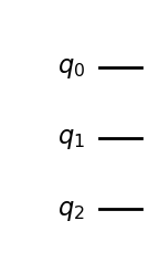
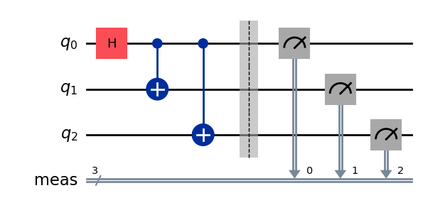
To build a quantum circuit, we start by specifying a number n of qubits for our circuits, where n can be as large as 127 or 156, depending on the underling QPU instance (see processor types). All n qubits are initialised in the |0⟩ state, so the initial state is |0 ⟩ⁿ . Here is how we initialise a circuit with 3 qubits in Qiskit.

from qiskit.circuit import QuantumCircuit

# A quantum circuit with three qubits
qc = QuantumCircuit(3)
qc.draw('mpl')

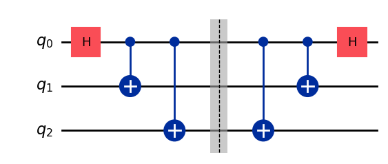
Next we can add operations on those qubits, in the form of quantum gates, which are unitary operations acting typically on one or two qubits. For instance let us add one Hadamard gate acting on the first qubit and two CX (aka CNOT) gates on the pairs of qubits (0, 1) and (0, 2).

# Hadamard gate on qubit 0.
qc.h(0)
# CX gates on qubits (0, 1) and (0, 2).
qc.cx(0, 1)
qc.cx(0, 2)

qc.draw('mpl')

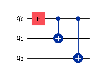
We obtain a 3-qubit circuit preparing the state

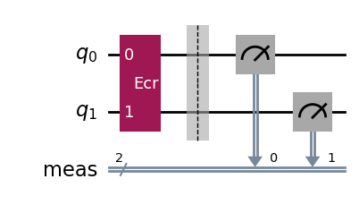
To measure the output qubits of the circuit, we add a measurement layer

qc.measure_all()
qc.draw('mpl')

It is possible to run the circuit and to get its output measured bits as a simulation with StatevectorSampleror on real quantum hardware with SamplerV2 . Let us see the output of a simulation first.

from qiskit.primitives import StatevectorSampler
from qiskit.transpiler.preset_passmanagers import generate_preset_pass_manager
from qiskit.visualization import plot_distribution

sampler = StatevectorSampler()
pm = generate_preset_pass_manager(optimization_level=1)
# Generate the ISA circuit
qc_isa = pm.run(qc)
# Run the simulator 10_000 times
num_shots = 10_000
result = sampler.run([qc_isa], shots=num_shots).result()[0]
# Collect and plot measurements
measurements= result.data.meas.get_counts()
plot_distribution(measurements)

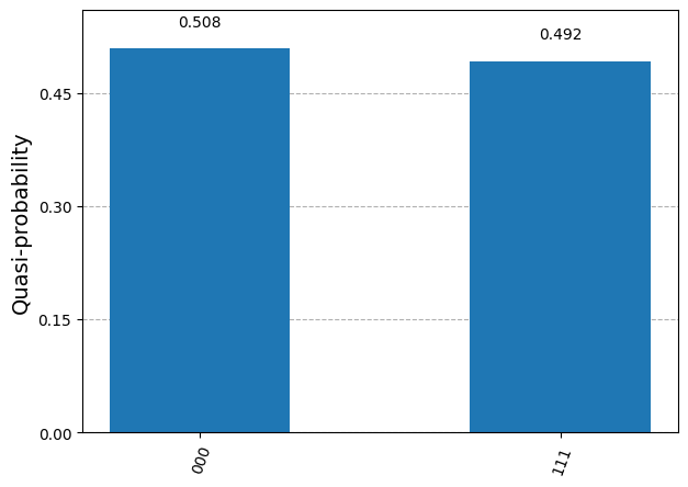
The measured bits are either (0,0,0) or (1,1,1), with approximate probability close to 0.5. This is precisely what we expect from sampling the 3-qubit state prepared by the circuit.

We now run the circuit on a QPU (see instructions on setting up an IBM Quantum account and retrieving your personal token)

from qiskit_ibm_runtime import QiskitRuntimeService
from qiskit_ibm_runtime import SamplerV2 as Sampler

service = QiskitRuntimeService(
    channel="ibm_quantum",
    token=<YOUR_TOKEN>, # use your IBM Quantum token here.
)
# Fetch a QPU to use
backend = service.least_busy(operational=True, simulator=False)
print(f"QPU: {backend.name}")
target = backend.target
sampler = Sampler(mode=backend)
pm = generate_preset_pass_manager(target=target, optimization_level=1)
# Generate the ISA circuit
qc_isa = pm.run(qc)
# Run the simulator 10_000 times
num_shots = 10_000
result = sampler.run([qc_isa], shots=num_shots).result()[0]
# Collect and plot measurements
measurements= result.data.meas.get_counts()
plot_distribution(measurements)

QPU: ibm_brisbane

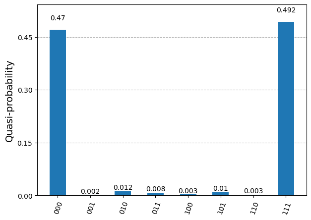
The measured bits are similar to those of the simulation, but now we see a few occurrences of the bit triplets (0,0,1), (0,1,0), (1,0,0), (0,1,1), (1,0,1) and (1,1,0). Those measurements should not occur from sampling the 3-qubit state prepared by the chosen circuit. They correspond to quantum errors occurring while running the circuit on the QPU.

We would like to quantify the error rate somehow, but it is not obvious how to do it. In quantum computations, what we really care about is that the qubit quantum state prepared by the circuit is the correct state. The measurements which are not (0,0,0) or (1,1,1) indicate errors in the state preparation, but this is not all. The measurements (0,0,0) and (1,1,1) could also be the result of incorrectly prepared states, e.g. the state (|0,0,0⟩ + |0,0,1⟩)/√2 can produce the output (0,0,0). Actually, it seems very likely that a few of the “correct” measurements come from incorrect 3-qubit states.

To understand this “noise” in the state preparation we need the formalism of density matrices to represent quantum states.

Density matrices and state fidelity

The state of an n-qubit circuit with incomplete information is represented by a 2ⁿ× 2ⁿ positive semi-definite hermitian matrix with trace equal to 1, called the density matrix ρ. Each diagonal element corresponds to the probability pᵢ of measuring one of the 2ⁿ possible states in a projective measurement, pᵢ = ⟨ψᵢ| ρ |ψᵢ⟩. The off-diagonal elements in ρ do not really have a physical interpretation, they can be set to zero by a change of basis states. In the computational basis, i.e. the standard basis |bit₀, bit₁, …, bitₙ⟩, they encode the entanglement properties of the state. Vector states |ψ⟩ describing the possible quantum states of the qubits have density matrices ρ = |ψ⟩⟨ψ|, whose eigenvalues are all 0, except for one eigenvalue, which is equal to 1. They are called pure states. Generic density matrices represent probabilistic quantum states of the circuit and have eigenvalues between 0 and 1. They are called mixed states. To give an example, a circuit which is in a state |ψ₁⟩ with probability q and in a state |ψ₂⟩ with probability 1-q is represented by the density matrix ρ = q|ψ₁⟩⟨ψ₁| + (1-q)|ψ₂⟩⟨ψ₂|.

In real quantum hardware, qubits are subject to all kinds of small unknown interactions with the environment, leading to a “loss of information”. This is the source of an incoherent quantum noise. Therefore, when applying gates to qubits or even when preparing the initial state, the quantum state of qubits cannot be described by a pure state, but ends up in a mixed state, which we must describe with a density matrix ρ. Density matrices provide a convenient way to describe quantum circuits in isolation, abstracting the complex and unknown interactions with the environment.

To learn more about density matrix representation of quantum states, you can look at any quantum information course. The excellent Qiskit lecture on this topic is available on YouTube.

For a single qubit, the density matrix, in the computational basis (i.e. the basis {|0⟩, |1⟩}), is a 2×2 matrix

with p₀ = ⟨0|ρ|0⟩ the probability to measure 0, p₁ = 1 — p₀ = ⟨1|ρ|1⟩ the probability to measure 1, and c is a complex number bounded by |c|² ≤ p₀p₁. Pure states have eigenvalues 0 and 1, so their determinant is zero, and they saturate the inequality with |c|² = p₀p₁.

In the following, we will consider quantum circuits with a few qubits and we will be interested in quantifying how close the output state density matrix ρ is from the expected (theoretical) output density matrix ρ₀. For a single qubit state, we could think about comparing the values of p₀, p₁ and c, provided we are able to measure them, but in a circuit with more qubits and a larger matrix ρ, we would like to come up with a single number quantifying how close ρ and ρ₀ are. Quantum information theory possesses such quantity. It is called state fidelity and it is defined by the slightly mysterious formula

The state fidelity F is a real number between 0 an 1, 0 ≤ F ≤ 1, with F = 1 corresponding to having identical states ρ = ρ₀ , and F = 0 corresponding to ρ and ρ₀ having orthogonal images. Although it is not so obvious from the definition, it is a symmetric quantity, F(ρ,ρ₀) = F(ρ₀,ρ).

In quantum circuit computations, the expected output state ρ₀ is always a pure state ρ₀ = |ψ₀⟩⟨ψ₀| and, in this case, the state fidelity reduces to the simpler formula

which has the desired interpretation as the probability for the state ρ to be measured in the state |ψ₀⟩ (in a hypothetical experiment implementing a projective measurement onto the state |ψ₀⟩ ).

In the noise-free case, the produced density matrix is ρ = ρ₀ = |ψ₀⟩⟨ψ₀| and the state fidelity is 1. In the presence of noise the fidelity decreases, F < 1.

In the remainder of this discussion, our goal will be to measure the state fidelity F of simple quantum circuit in Qiskit, or, more precisely, to estimate a lower bound F̃ < F.

State fidelity estimation in quantum circuits

To run quantum circuits on QPUs and collect measurement results, we define the function run_circuit .

def run_circuit(
        qc: QuantumCircuit, 
        service: QiskitRuntimeService = service, 
        num_shots: int = 100,
    ) -> tuple[dict[str, int], QuantumCircuit]:
    """Runs the circuit on backend 'num_shots' times. Returns the counts of 
    measurements and the ISA circuit."""
    # Fetch an available QPU
    backend = service.least_busy(operational=True, simulator=False)
    target = backend.target
    pm = generate_preset_pass_manager(target=target, optimization_level=1)
    
    # Add qubit mesurement layer and compute ISA circuit
    qc_meas = qc.measure_all(inplace=False)
    qc_isa = pm.run(qc_meas)

    # Run the ISA circuit and collect results
    sampler = Sampler(mode=backend)
    result = sampler.run([qc_isa], shots=num_shots).result()
    dist = result[0].data.meas.get_counts()

    return dist, qc_isa

The ISA (Instruction Set Architecture) circuit qc_isa returned by this function is essentially a rewriting of the provided circuit in terms of the physical gates available on the QPU, called basis gates. This is the circuit that is actually constructed and run on the hardware.

Note: The run_circuit function starts by fetching an available QPU. This is convenient to avoid waiting too long for the computation to be processed. However this also means that we use different QPUs each time we call the function. This is not ideal, as it is possible that different QPUs have different level of quantum noise. However, in practice, the fetched QPUs all turned out to be in the Eagle family and we present noise estimation only for this QPU family. To keep our analysis simple, we just assume that the level of quantum noise among the possible QPU instances is stable. The interested reader could try to find whether there are differences between instances.

Bare |0⟩ state

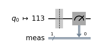
Let us start with the simplest circuit, which comprises only an initialised qubit |0⟩ without any gate operation.

# A quantum circuit with a single qubit |0>
qc = QuantumCircuit(1)
dist, qc_isa = run_circuit(qc, num_shots=100_000)
qc_isa.draw(output="mpl", idle_wires=False, style="iqp")

import numpy as np

def print_results(dist: dict[str, int]) -> None:
    print(f"Measurement counts: {dist}")
    num_shots = sum([dist[k] for k in dist])
    for k, v in dist.items():
        p = v / num_shots
        # 1% confidence interval estimate for a Bernoulli variable
        delta = 2.575 * np.sqrt(p*(1-p)/num_shots)
        print(f"p({k}): {np.round(p, 4)}  ± {np.round(delta, 4)}")

print_results(dist)

Measurement counts: {'0': 99661, '1': 339}
p(0) = 0.9966 ± 0.0005
p(1) = 0.0034 ± 0.0005

We get a small probability, around 0.3%, to observe the incorrect result 1. The interval estimate “± 0.0005” refers to a 1% confidence interval estimate for a Bernoulli variable.

The fidelity of the output state ρ, relative to the ideal state |0⟩, is F = ⟨0|ρ|0⟩ = p₀. We have obtained an estimate of 0.9966 ± 0.0005 for p₀ from the repeated measurements of the circuit output state. But the measurement operation is a priori imperfect (it has its own error rate). It may add a bias to the p₀ estimate. We assume that these measurement errors tend to decrease the estimated fidelity by incorrect measurements of |0⟩ states. In this case, the estimated p₀ will be a lower bound on the true fidelity F:

F > F̃ = 0.9966 ± 0.0005

Note: We have obtained estimated probabilities p₀, p₁ for the diagonal components of the single-qubit density matrix ρ. We also have an estimated bound on the off-diagonal component |c| < √(p₀ p₁) ~ 0.06. To get an actual estimate for c, we would need to run a circuit some gates and design a more complex reasoning.

Basis gates

Qiskit offers a large number of quantum gates encoding standard operations on one or two qubits, however all these gates are encoded in the QPU hardware with combinations of a very small set of physical operations on the qubits, called basis gates.

There are three single-qubit basis gates: X, SX and RZ(λ) and one two-qubit basis gate: ECR. All other quantum gates are constructed from these building blocks. The more basis gates are used in a quantum circuit, the larger is the quantum noise. We will analyse the noise resulting from applying these basis gates in isolation, when possible, or with a minimal number of basis gates, to get a sense of quantum noise in the current state of QPU computations.

X gate

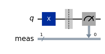
We consider the circuit made of a single qubit and an X gate. The output state, in the absence of noise, is X|0⟩ = |1⟩.

# Quantum circuit with a single qubit and an X gate. 
# Expected output state X|0> = |1>.
qc = QuantumCircuit(1)
qc.x(0)

dist, qc_isa = run_circuit(qc, num_shots=100_000)
qc_isa.draw(output="mpl", idle_wires=False, style="iqp")

print_results(dist)

Measurement counts: {'1': 99072, '0': 928}
p(0) = 0.0093 ± 0.0008
p(1) = 0.9907 ± 0.0008

The state fidelity of the output state ρ, relative to the ideal state |1⟩, is

F = ⟨1|ρ|1⟩ = p₁ > F̃ = 0.9907 ± 0.0008

where we assumed again that the measurement operation lower the estimated fidelity and we get a lower bound F̃ on the fidelity.

We observe that the fidelity is (at least) around 99.1%, which is a little worse than the fidelity measured without the X gate. Indeed, adding a gate to the circuit should add noise, but there can be another effect contributing to the degradation of the fidelity, which is the fact that the |1⟩ state is a priori less stable than the |0⟩ state and so the measurement of a |1⟩ state itself is probably more noisy. We will not discuss the physical realisation of a qubit in IBM QPUs, but one thing to keep in mind is that the |0⟩ state has lower energy than the |1⟩ state, so that it is quantum mechanically more stable. As a result, the |1⟩ state can decay to the |0⟩ state through interactions with the environement.

SX gate

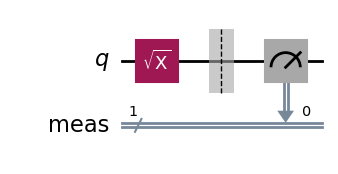
We now consider the SX gate, i.e. the “square-root X” gate, represented by the matrix

It transforms the initial qubit state |0⟩ into the state

# Quantum circuit with a single qubit and an SX gate. 
qc = QuantumCircuit(1)
qc.sx(0)

dist, qc_isa = run_circuit(qc, num_shots=100_000)
qc_isa.draw(output="mpl", idle_wires=False, style="iqp")

print_results(dist)

Measurement counts: {'1': 50324, '0': 49676}
p(0) = 0.4968 ± 0.0041
p(1) = 0.5032 ± 0.0041

We observe roughly equal distributions of zeros and ones, which is as expected. But we face a problem now. The state fidelity cannot be computed from these p₀ and p₁ estimates. Indeed, the fidelity of the output state ρ, relative to the ideal output state SX|0⟩ is

Therefore, to get an estimate of F, we also need to measure c, or rather its imaginary part Im(c). Since there is no other measurement we can do on the SX gate circuit, we need to consider a circuit with more gates to evaluate F, but more gates also means more sources of noise.

One simple thing we can do is to add either another SX gate or an SX⁻¹ gate. In the former case, the full circuit implements the X operation and the expected final state |1⟩, while in the latter case, the full circuit implements the identity operation and the expected final state is |0⟩.

Let us consider the case of adding an SX gate: the density matrix ρ produced by the first SX gate gets transformed into

leading to p’₁ = 1/2— Im(c) = F, in the ideal case when the second SX gate is free of quantum noise. In practice the SX gate is imperfect and we can only measure p’₁ = 1/2 — Im(c) — δp = F — δp, where δp is due to the noise from the second SX gate. Although it is theoretically possible that the added noise δp combines with the noise introduced by the first SX gate and results in a smaller combined noise, we will assume that no such “happy” cancelation happens, so that we have δp>0. In this case, p’₁ < F gives us a lower bound on the state fidelity F.

qc = QuantumCircuit(1)
qc.sx(0)
qc.barrier() # Prevents simplification of the circuit during transpilation.
qc.sx(0)

dist, qc_isa = run_circuit(qc, num_shots=100_000)

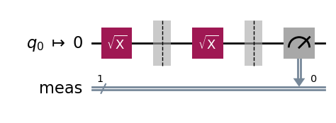
print_results(dist)

Measurement counts: {'1': 98911, '0': 1089}
p(1): 0.9891  ± 0.0008
p(0): 0.0109  ± 0.0008

We obtain a lower bound F > p’₁ = 0.9891 ± 0.0008, on the fidelity of the output state ρ for the SX-gate circuit, relative to the ideal output state SX|0⟩.

We could have considered the two-gate circuit with an SX gate followed by an SX⁻¹ gate instead. The SX⁻¹ gate is not a basis gate. It is implemented in the QPU as SX⁻¹ = RZ(-π) SX RZ(-π). We expect this setup to add more quantum noise due the presence of more basis gates, but in practice we have measured a higher (better) lower bound F̃. The interested reader can check this as an exercise. We believe this is due to the fact that the unwanted interactions with the environment tend to bring the qubit state to the ground state |0⟩, improving incorrectly the lower bound estimate, so we do not report this alternative result.

RZ(λ) gate

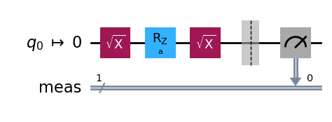
Next we consider the RZ(λ) gate. The RZ(λ) gate is a parametrised gate implementing a rotation around the z-axis by an angle λ/2.

Its effect on the initial qubit |0⟩ is only to multiply it by a phase exp(-iλ/2), leaving it in the same state. In general, the action of RZ(λ) on the density matrix of a single qubit is to multiply the off-diagonal coefficient c by exp(iλ), leaving the p₀ and p₁ values of the state unchanged. To measure a non-trivial effect of the RZ(λ) gate, one needs to consider circuits with more gates. The simplest is to consider the circuit composing the three gates SX, RZ(λ) and SX, preparing the state

The expected p(0) and p(1) values are

Qiskit offers the possibility to run parametrised quantum circuits by specifying an array of parameter values, which, together with the ISA circuit, define a Primitive Unified Bloc (PUB). The PUB is then passed to the sampler to run the circuit with all the specified parameter values.

from qiskit.primitives.containers.sampler_pub_result import SamplerPubResult

def run_parametrised_circuit(
        qc: QuantumCircuit, 
        service: QiskitRuntimeService = service, 
        params: np.ndarray | None = None,
        num_shots: int = 100,
    ) -> tuple[SamplerPubResult, QuantumCircuit]:
    """Runs the parametrised circuit on backend 'num_shots' times. 
    Returns the PubResult and the ISA circuit."""
    # Fetch an available QPU
    backend = service.least_busy(operational=True, simulator=False)
    target = backend.target
    pm = generate_preset_pass_manager(target=target, optimization_level=1)
    
    # Add mesurement layer
    qc_meas = qc.measure_all(inplace=False)
    # Define ISA circuit and PUB
    pm = generate_preset_pass_manager(target=target, optimization_level=1)
    qc_isa = pm.run(qc_meas)
    sampler_pub = (qc_isa, params)
    
    # Run the circuit
    result = sampler.run([sampler_pub], shots=num_shots).result()
    return result[0], qc_isa

from qiskit.circuit import Parameter

# Circuit preparing the state SX.RZ(a).SX|0> = sin(a/2)|0> + cos(a/2)|1>.
qc = QuantumCircuit(1)
qc.sx(0)
qc.rz(Parameter("a"), 0)
qc.sx(0)

# Define parameter range
params = np.linspace(0, 2*np.pi, 21).reshape(-1, 1)
# Run parametrised circuit
pub_result, qc_isa = run_parametrised_circuit(qc, params=params, num_shots=10_000)

qc_isa.draw(output="mpl", idle_wires=False, style="iqp")

bit_array = pub_result.data.meas.bitcount()
print(f"bit_array shape: {bit_array.shape}")
p0 = (bit_array.shape[1] - bit_array.sum(axis=1)) / bit_array.shape[1]
p1 = bit_array.sum(axis=1) / bit_array.shape[1]
print(f"p(0): {p0}")
print(f"p(1): {p1}")

bit_array shape: (21, 10000)
p(0): [0.0031 0.0265 0.095  0.2095 0.3507 0.4969 0.6567 0.7853 0.9025 0.9703
 0.9983 0.976  0.901  0.7908 0.6543 0.5013 0.3504 0.2102 0.0982 0.0308
 0.0036]
p(1): [0.9969 0.9735 0.905  0.7905 0.6493 0.5031 0.3433 0.2147 0.0975 0.0297
 0.0017 0.024  0.099  0.2092 0.3457 0.4987 0.6496 0.7898 0.9018 0.9692
 0.9964]

import matplotlib.pyplot as plt

x = params/(2*np.pi)
plt.scatter(x, p0)
plt.scatter(x, p1)
plt.plot(x, np.sin(np.pi*x)**2, linestyle="--")
plt.plot(x, np.cos(np.pi*x)**2, linestyle="--")
plt.xlabel("λ/2π")
plt.ylabel("Estimated probabilities")
plt.legend(["p(0)", "p(1)", "sin(λ/2)^2", "cos(λ/2)^2"])
plt.show()

We see that the estimated probabilities (blue and orange dots) agree very well with the theoretical probabilities (blue and orange lines) for all tested values of λ.

Here again, this does not give us the state fidelity. We can give a lower bound by adding another sequence of gates SX.RZ(λ).SX to the circuit, bringing back the state to |0⟩. As in the case of the SX gate of the previous section, the estimated F̃ := p’₀ from this 6-gate circuit gives us a lower bound on the fidelity of the F of the 3-gate circuit, assuming the extra gates lower the output state fidelity.

Let us compute this lower bound F̃ for one value, λ = π/4.

# Circuit implementing SX.RZ(π/4).SX.SX.RZ(π/4).SX|0> = |0>
qc = QuantumCircuit(1)
qc.sx(0)
qc.rz(np.pi/4, 0)
qc.sx(0)
qc.barrier()  # Prevents circuit simplifications.
qc.sx(0)
qc.rz(np.pi/4, 0)
qc.sx(0)

dist, qc_isa = run_circuit(qc, num_shots=100_000)
qc_isa.draw(output="mpl", idle_wires=False, style="iqp")

dist = pub_result.data.meas.get_counts()
print_results(dist)

Measurement counts: {'0': 99231, '1': 769}
p(0): 0.9923  ± 0.0007
p(1): 0.0077  ± 0.0007

We find a pretty high lower bound estimate F̃ = 0.9923 ± 0.0007.

Digression: a lower bound estimate procedure

The above case showed that we can estimate a lower bound on the fidelity F of the output state of a circuit by extending the circuit with its inverse operation and measuring the probability of getting the initial state back.

Let us consider an n-qubit circuit preparing the state |ψ⟩ = U|0,0, … ,0⟩. The state fidelity of the output density matrix ρ is given by

U⁻¹ρU is the density matrix of the circuit composed of a (noisy) U gate and a noise-free U⁻¹ gate. F is equal to the fidelity of the |0,0, …, 0⟩ state of this 2-gate circuit. If we had such a circuit, we could sample it and measure the probability of (0, 0, …, 0) as the desired fidelity F.

In practice we don’t have a noise-free U⁻¹ gate, but only a noisy U⁻¹ gate. By sampling this circuit (noisy U, followed by noisy U⁻¹) and measuring the probability of the (0, 0, …, 0) outcome, we obtain an estimate F̃ of F — δp, with δp the noise overhead added by the U⁻¹ operation (and the measurement operation). Under the assumption δp>0, we obtain a lower bound F > F̃. This assumption is not necessarily true because the noisy interactions with the environment likely tend to bring the qubits to the ground state |0,0, …, 0⟩, but for “complex enough” operations U, this effect should be subdominant relative to the noise introduced by the U⁻¹ operation. We have used this approach to estimate the fidelity in the SX.RZ(λ).SX circuit above. We will use it again to estimate the fidelity of the ECR-gate and the 3-qubit state from the initial circuit we considered.

ECR gate

The ECR gate (Echoed Cross-Resonance gate) is the only two-qubit basis gate in the Eagle family of IBM QPUs (other families support the CZ or CX gate instead, see tables of gates). It is represented in the computational basis by the 4×4 matrix

Its action on the initial 2-qubit state is

The measurements of a noise-free ECR gate circuit are (0,1) with probability 1/2 and (1,1) with probability 1/2. The outcome (0,0) and (1,0) are not possible in the noise-free circuit.

qc = QuantumCircuit(2)
qc.ecr(0, 1)
dist, qc_isa = run_circuit(qc, num_shots=100_000)

qc_isa.draw(output="mpl", idle_wires=False, style="iqp")

print_results(dist)

Measurement counts: {'11': 49254, '01': 50325, '00': 239, '10': 182}
p(11): 0.4925  ± 0.0041
p(01): 0.5032  ± 0.0041
p(00): 0.0024  ± 0.0004
p(10): 0.0018  ± 0.0003

We observe a distribution of measured classical bits roughly agreeing with the expected ideal distribution, but the presence of quantum errors is revealed by the presence of a few (0,0) and (1, 0) outcomes.

The fidelity of the output state ρ is given by

As in the case of the SX-gate circuit, we cannot directly estimate the fidelity of the ρ state prepared by the ECR-gate circuit by measuring the output bits of the circuit, since it depends on off-diagonal terms in the ρ matrix.

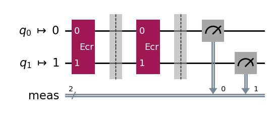
Instead we can follow the procedure described in the previous section and estimate a lower bound on F by considering the circuit with an added ECR⁻¹ gate. Since ECR⁻¹ = ECR, we consider a circuit with two ECR gates.

qc = QuantumCircuit(2)
qc.ecr(0, 1)
qc.barrier()  # Prevents circuit simplifications.
qc.ecr(0, 1)
dist, qc_isa = run_circuit(qc, num_shots=100_000)
qc_isa.draw(output="mpl", idle_wires=False, style="iqp")

print_results(dist)

Measurement counts: {'00': 99193, '01': 153, '10': 498, '11': 156}
p(00): 0.9919  ± 0.0007
p(01): 0.0015  ± 0.0003
p(10): 0.005  ± 0.0006
p(11): 0.0016  ± 0.0003

We find the estimated lower bound F > 0.9919 ± 0.0007 on the ρ state prepared by the ECR-gate circuit.

3-qubit state fidelity

To close the loop, in our final example, let us compute a lower bound on the state fidelity of the 3-qubit state circuit which we considered first. Here again, we add the inverse operation to the circuit, bringing back the state to |0,0,0⟩ and measure the circuit outcomes.

qc = QuantumCircuit(3)
qc.h(0)
qc.cx(0, 1)
qc.cx(0, 2)
qc.barrier(). # Prevents circuit simplifications.
qc.cx(0, 2)
qc.cx(0, 1)
qc.h(0)
qc.draw('mpl')

dist, qc_isa = run_circuit(qc, num_shots=100_000)
qc_isa.draw(output="mpl", idle_wires=False, style="iqp")

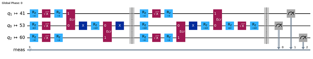
print_results(dist)

Measurement counts: {'000': 95829, '001': 1771, '010': 606, '011': 503, '100': 948, '101': 148, '111': 105, '110': 90}
p(000): 0.9583  ± 0.0016
p(001): 0.0177  ± 0.0011
p(010): 0.0061  ± 0.0006
p(011): 0.005  ± 0.0006
p(100): 0.0095  ± 0.0008
p(101): 0.0015  ± 0.0003
p(111): 0.001  ± 0.0003
p(110): 0.0009  ± 0.0002

We find the fidelity lower bound F̃ = p’((0,0,0)) = 0.9583 ± 0.0016 for the 3-qubit state circuit.

Summary of results and discussion

Let us summarise our results in a table of fidelity lower bounds for the circuits we considered, using IBM QPUs.

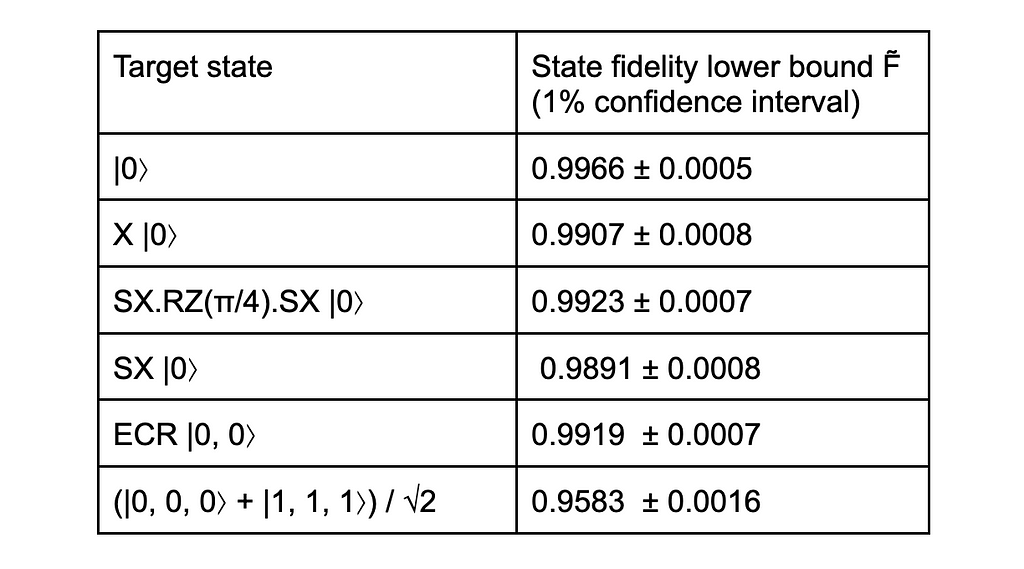
We find that the fidelity of states produced by circuits with a minimal number of basis gate is around 99%, which is not a small achievement. As we add more qubits and gates, the fidelity decreases, as we see with the 96% fidelity for the 3-qubit state, whose circuit has 13 basis gates. With more qubits and circuit depth, the fidelity would decrease further, to the point that the quantum computation would be completely unreliable. Nevertheless, these results look quite encouraging for the future of quantum computing.

It is likely that more accurate and rigorous methods exist to evaluate the fidelity of the state produced by a quantum circuit, giving more robust bounds. We are just not aware of them. The main point was to provide hands-on examples of Qiskit circuit manipulations for beginners and to get approximate quantum noise estimates.

While we have run a number of circuits to estimate quantum noise, we have only scratched the surface of the topic. There are many ways to go further, but one important idea to make progress is to make assumptions on the form of the quantum noise, namely to develop a model for a quantum channel representing the action of the noise on a state. This would typically involve a separation between “coherent” noise, preserving the purity of the state, which can be described with a unitary operation, and “incoherent” noise, representing interactions with the environment. The Qiskit Summer School lecture on the topic provides a gentle introduction to these ideas.

Finally, here are a few reviews related to quantum computing, if you want to learn more on this topic. [1] is an introduction to quantum algorithms. [2] is a review of quantum mitigation techniques for near-term quantum devices. [3] is an introduction to quantum error correction theory. [4] is a review of quantum computing ideas and physical realisation of quantum processors in 2022, aimed at a non-scientific audience.

Thanks for getting to the end of this blogpost. I hope you had some fun and learned a thing or two.

Unless otherwise noted, all images are by the author

[1] Blekos, Kostas and Brand, Dean and Ceschini, Andrea and Chou, Chiao-Hui and Li, Rui-Hao and Pandya, Komal and Summer, Alessandro, Quantum Algorithm Implementations for Beginners (2023), Physics Reports Volume 1068, 2 June 2024.

[2] Cai, Zhenyu and Babbush, Ryan and Benjamin, Simon C. and Endo, Suguru and Huggins, William J. and Li, Ying and McClean, Jarrod R. and O’Brien, Thomas E., Quantum error mitigation (2023), Reviews of Modern Physics 95, 045005.

[3] J. Roffe, Quantum error correction: an introductory guide (2019), Contemporary Physics, Oct 2019.

[3] A. K. Fedorov, N. Gisin, S. M. Beloussov and A. I. Lvovsky, Quantum computing at the quantum advantage threshold: a down-to-business review (2022).

---

Measuring Quantum Noise in IBM Quantum Computers was originally published in Towards Data Science on Medium, where people are continuing the conversation by highlighting and responding to this story.

Even with zero math background

Do you want to become a Data Scientist or machine learning engineer, but you feel intimidated by all the math involved? I get it. I’ve been there.

I dropped out of High School after 10th grade, so I never learned any math beyond trigonometry in school. When I started my journey into Machine Learning, I didn’t even know what a derivative was.

Fast forward to today, and I’m an Applied Scientist at Amazon, and I feel pretty confident in my math skills.

I’ve picked up the necessary math along the way using free resources and self-directed learning. Today I’m going to walk you through some of my favorite books, courses, and YouTube channels that helped me get to where I am today, and I’ll also share some tips on how to study effectively and not waste your time struggling and being bored.

Do You Even Need to Know Math for ML?

First, let’s address a common question: Do you even really need to know the math to work in ML?

The short answer is: it depends on what you want to do.

For research-heavy roles where you’re creating new ML algorithms, then yes, you obviously need to know the math. But if you’re asking yourself if you need to learn math, chances are that’s not the kind of job you’re looking for…

But for practitioners — most of us in the industry — you can often be totally competent without knowing all the underlying details, especially as a beginner.

At this point, libraries like numpy, scikit-learn, and Tensorflow handle most of the heavy lifting for you. You don’t need to know the math behind gradient descent to deploy a model to production.

If you’re a beginner trying to get into ML, in my opinion it is not strategic to spend a bunch of time memorizing formulas or studying linear algebra — you should be spending that time building things. Train a simple model. Explore your data. Build a pipeline that predicts something fun.

That said, there are moments where knowing the math really helps. Here are a few examples:

Imagine you’re training a model and it’s not converging. If you understand concepts like gradients and optimization functions, you’ll know whether to adjust your learning rate, try a different optimizer, or tweak your data preprocessing.

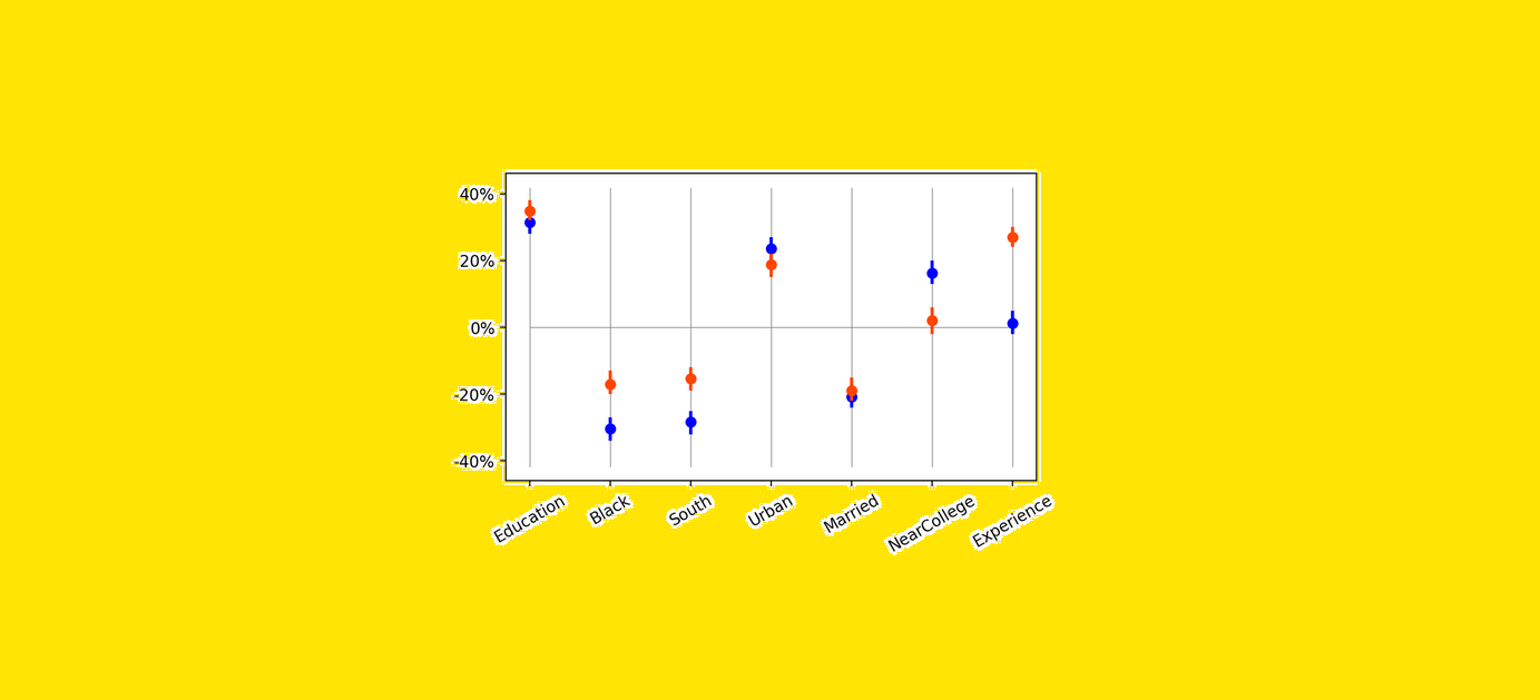
Or, let’s say you’re running a linear regression, and you’re interpreting the coefficients. Without math knowledge, you might miss problems like multicollinearity, which makes those coefficients unreliable. Then you make incorrect conclusions from the data and cost the company millions and lose your job! Just kidding. Kind of. We do need to be careful when making business decisions from the models we build.

So, while you can (and should) get started without deep math knowledge, it’s definitely still reasonable to build your comfort with math over time.

Once you’re hands-on, you’ll start encountering problems that naturally push you to learn more. When you need to debug or explain your results, that’s when the math will start to click, because it’s connected to real problems.

So seriously, don’t let the fear of math stop you from starting. You don’t need to learn it all upfront to make progress. Get your hands dirty with the tools, build your portfolio, and let math grow as a skill alongside your practical knowledge.

What to Learn

Alright, now let’s talk about what to learn when you’re building your math foundation for Machine Learning jobs.

First, linear algebra.

Linear algebra is fundamental for Machine Learning, especially for deep learning. Many models rely on representing data and computations as matrices and vectors. Here’s what to prioritize:

• Matrices and Vectors: Think of matrices as grids of numbers and vectors as lists. Data is often stored this way, and operations like addition, multiplication, and dot products are central to how models process that information.
• Determinants and Inverses: Determinants tell you whether a matrix can be inverted, which is used in optimization problems and solving systems of equations.
• Eigenvalues and Eigenvectors: These are key to understanding variance in data and are the foundation of techniques like Principal Component Analysis, which helps reduce dimensionality in datasets.
• Lastly, Matrix Decomposition: Methods like Singular Value Decomposition (SVD) are used in recommendation systems, dimensionality reduction, and data compression.

Now we’re on to basic calculus.

Calculus is core to understanding how models learn from data. But, we don’t need to worry about solving complex integrals — it’s just about grasping a few key ideas:

• First, derivatives and gradients: Derivatives measure how things change, and gradients (which are multidimensional derivatives) are what power optimization algorithms like gradient descent. These help models adjust their parameters to minimize error.
• The Chain Rule is central to neural networks. It’s how backpropagation works — which is the process of figuring out how much each weight in the network contributes to the overall error so the model can learn effectively.
• Lastly, optimization basics: Concepts like local vs. global minima, saddle points, and convexity are important to understand why some models get stuck and others find the best solutions.

Lastly, statistics and probability.

Statistics and probability are the bread and butter of understanding data. While they’re more associated with data science, there’s definitely a lot of value for ML as well. Here’s what you need to know:

• Distributions: Get familiar with common ones like normal, binomial, and uniform. The normal distribution, in particular, pops up everywhere in data science and ML.
• Variance and covariance: Variance tells you how spread out your data is, while covariance shows how two variables relate. These concepts are really important for feature selection and understanding your data’s structure.
• Bayes’ Theorem: While it has kind of an intimidating name, Bayes’ theorem is a pretty simple but powerful tool for probabilistic reasoning. It’s foundational for algorithms like Naive Bayes — big surprise — which is used for things like spam detection, as well as for Bayesian optimization for hyperparameter tuning.
• You’ll also want to understand Maximum Likelihood Estimation (MLE), which helps estimate model parameters by finding values that maximize the likelihood of your data. It’s a really fundamental concept in algorithms like logistic regression.
• Finally, sampling and conditional probability: Sampling lets you work with subsets of data efficiently, and conditional probability is essential for understanding relationships between events, especially in Bayesian methods.

Now, this is definitely not exhaustive, but I think it’s a good overview of the common concepts you’ll need to know to do a good job as a data scientist or MLE.

Next up, I’ll share the best resources to learn these concepts without it being stressful or overwhelming.

Resources

Personally, I would highly recommend starting with a visual and intuitive understanding of the key concepts before you start reading difficult books and trying to solve equations.

For Linear Algebra and Calculus, I cannot speak highly enough about 3blue1brown’s Essence of Linear Algebra and Essence of Calculus series. These videos give a solid introduction to what is actually being measured and manipulated when we use these mathematical approaches. More importantly, they show, let’s say, the beauty in it? It’s strange to say that math videos could be inspirational, but these ones are.

For statistics and probability, I am also a huge fan of StatQuest. His videos are clear, engaging, and just a joy to watch. StatQuest has playlists with overviews on core stats and ML concepts.

So, start there. Once you have a visual intuition, you can start working through more structured books or courses.

There are lots of great options here. Let’s go through a few that I personally used to learn:

I completed the Mathematics for Machine Learning Specialization from Imperial College London on Coursera when I was just starting out. The specialization is divided into three courses: Linear Algebra, Multivariate Calculus, and a last one on Principal Component Analysis. The courses are well-structured and include a mix of video lectures, quizzes, and programming assignments in Python. I found the course to be a bit challenging as a beginner, but it was a really good overview and I passed with a bit of effort.

DeepLearning.AI also recently released a Math for ML Specialization on Coursera. This Specialization also has courses on Linear Algebra and Calculus, but instead of PCA the final course focuses on Stats and Probability. I’m personally working through this Specialization right now, and overall I’m finding it to be another really great option. Each module starts with a nice motivation for how the math connects to an applied ML concept, it has coding exercises in Python, and some neat 3D tools to mess around with to get a good visual understanding of the concepts.

If you prefer learning from books, I have some suggestions there too. First up, if you like anime or nerdy stuff, oh boy do I have a recommendation for you.

Did you know they have manga math books?

The Manga Guide to Calculus

The Manga Guide to Linear Algebra

The Manga Guide to Statistics

These are super fun. I can’t say that the instructional quality is world-class or anything, but they are cute and engaging, and they made me not dread reading a math book.

The next level up would be “real” math books. These are some of the best:

The Mathematics for Machine Learning ebook by Deisenroth and colleagues is a great comprehensive resource available for free for personal use. It covers key topics we’ve already discussed like Linear Algebra, Calculus, Probability, and Optimization, with a focus on how these concepts apply to machine learning algorithms. It’s relatively beginner-friendly and is generally regarded as one of the best books for learning this material.

Next, Practical Statistics for Data Scientists is another well-loved resource that includes code examples in Python and R.

How to Study

Now, before we actually start studying, I think it’s important to spend a little bit of time thinking really deeply about why you even want to do this. Personally, I find that if I’m studying just because I feel like I “should,” or because it’s some arbitrary assignment, I get distracted easily and don’t actually retain much.

Instead, I try to connect to a deeper motivation. Personally, right now I have a really basic motivation: I want to earn a lot of money so that I can take care of everyone I love. I have this opportunity to push myself and make sure everyone is safe and cared for, now and in the future. This isn’t to put extra pressure on myself, but actually just a way that works for me to get excited that I have this opportunity to learn and grow and hopefully help others along the way. Your motivation might be totally different, but whatever it is, try to tie this work to a larger goal.

In terms of strategies for optimizing your study time, I have found that one of the most effective methods is writing notes in my own words. Don’t just copy definitions or formulas — take time to summarize concepts as if you were explaining them to someone else — or, to future you. For example, if you’re learning about derivatives, you might write, “A derivative measures how a function changes as its input changes.” This forces you to actively process the material.

Relatedly, when it comes to math formulas, don’t just stare at them — translate them into plain English — or whatever spoken language you prefer. For instance, take the equation y=mx+b: you might describe m as “the slope that shows how steep the line is,” and b as “the point where the line crosses the y-axis.” So, the final formula, might be, “The value of y (the output) is determined by taking the slope (m), multiplying it by x (the input), and then adding b (the starting point where the line intersects the y-axis).”

You can even use your notes as like a personal blog. Writing short posts about what you’ve learned is a really solid way to clarify your understanding, and teaching others (even if no one reads it) solidifies the material in your own mind. Plus, sharing your posts on Medium or LinkedIn not only potentially helps others but also allows you to build a portfolio showcasing your learning journey.

Also trust me, when it’s interview time you’ll be happy you have these notes! I use my own study notes all the time.

This next piece of advice I have might not be super fun, but I also recommend not using just one resource. Personally I’ve had a lot of success from taking many different courses, and kind of throwing all my notes together at first. Then, I’ll write a blog like I was just talking about that summarizes all of my learnings.

There are a couple of advantages to this approach: First, repetition helps you retain things. If I see a concept multiple times, explained from multiple angles, I’m much more likely to actually get what’s going on and remember that for longer than a day. Plus, not only do I see the information presented to me multiple times, I’m writing the concepts out in my own words multiple times, including that final time where I synthesize it all and get it ready to share with others — so I have to be really confident I actually got it by the end.

Finally, once you’ve built that foundation and get to the level of math where you can actually use it for stuff, I really recommend coding concepts from scratch. If you can code gradient descent or logistic regression using just numpy, you’re off to a really strong start.

Again, Math (Probably) Won’t Get You a Job

While I know at this point you’re super excited to start learning math, I do want to just circle back to the important fact that if you’re a beginner trying to get your first job, in my opinion math should not be the first thing you prioritize.

It is really unlikely that your math skills are what will get you a job as a data scientist or MLE.

Instead, prioritize gaining hands-on experience by working on projects and actually building stuff. Employers are far more interested in seeing what you can do with the tools and knowledge you already have than how many formulas you’ve memorized.

As you encounter challenges in your work, you’ll naturally be motivated to learn the math behind the algorithms. Remember, math is a tool to help you succeed, and shouldn’t be a barrier to getting started.

—

If you want more advice on how to break into data science, you can download a free 80+ page e-book on how to get your first data science job (learning resources, project ideas, LinkedIn checklist, and more): https://gratitudedriven.com/

Or, check out my YouTube channel!

Finally, just a heads up, there are affiliate links in this post. So, if you buy something I’ll earn a small commission, at no additional cost to you. Thank you for your support.

---

How To Learn Math for Machine Learning, Fast was originally published in Towards Data Science on Medium, where people are continuing the conversation by highlighting and responding to this story.

Tracing the roots of ChatGPT: GPT-1, the foundation of OpenAI’s LLMs

The GPT (Generative Pre-Training) model family, first introduced by OpenAI in 2018, is another important application of the Transformer architecture. It has since evolved through versions like GPT-2, GPT-3, and InstructGPT, eventually leading to the development of OpenAI’s powerful LLMs.

In other words: understanding GPT models is essential for anyone looking to dive deeper into the world of LLMs.

This is the first part of our GPT series, in which we will try to walk through the core concepts in GPT-1 as well as the prior works that have inspired it.

Below are the topics we will cover in this article:

Prior to GPT-1:

• The Pre-training and Finetuning Paradigm: the journey from CV to NLP.
• Previous Work: Word2vec, GloVe, and other methods using LM for pretraining.
• Decoder-only Transformer.
• Auto-regressive vs. Auto-encoding Language Models.

Core concepts in GPT-1:

• Key Innovations.
• Pre-training.
• Finetuning.

Prior to GPT-1

Pre-training and Finetuning

The pretraining + finetuning paradigm, which firstly became popular in Computer Vision, refers to the process of training a model using two stages: pretraining and then finetuning.

In pretraining stage, the model is trained on a large-scale dataset that related to the downstream task at hand. In Computer Vision, this is done usually by learning an image classification model on ImageNet, with its most commonly used subset ILSVR containing 1K categories, each has 1K images.

Although 1M images doesn’t sound like “large-scale” by today’s standard, ILSVR was truly remarkable in a decade ago and was indeed much much larger than what we could have for specific CV tasks.

Also, the CV community has explored a lot of ways to get rid of supervised pre-training as well, for example MoCo (by Kaiming He et al.) and SimCLR (by Ting Chen et al.), etc.

After pre-training, the model is assumed to have learnt some general knowledge about the task, which could accelerate the learning process on the downstream task.

Then comes to finetuning: In this stage, the model will be trained on a specific downstream task with high-quality labeled data, often in much smaller scale compared to ImageNet. During this stage, the model will pick up some domain-specific knowledge related to the task at-hand, which helps improve its performance.

For a lot of CV tasks, this pretraining + finetuning paradigm demonstrates better performance compared to directly training the same model from scratch on the limited task-specific data, especially when the model is complex and hence more likely to overfit on limited training data. Combined with modern CNN networks such as ResNet, this leads to a performance leap in many CV benchmarks, where some of which even achieve near-human performance.

Therefore, a natural question arises: how can we replicate such success in NLP?

Previous Explorations of Pretraining Prior to GPT-1

In fact, the NLP community never stops trying in this direction, and some of the efforts can date back to as early as 2013, such as Word2Vec and GloVe (Global Vectors for Word Representation).

Word2Vec

The Word2Vec paper “Distributed Representations of Words and Phrases and their Compositionality” was honored with the “Test of Time” award at NeurIPS 2023. It’s really a must-read for anyone not familiar with this work.

Today it feels so natural to represent words or tokens as embedding vectors, but this wasn’t the case before Word2Vec. At that time, words were commonly represented by one-hot encoding or some count-based statistics such as TD-IDF (term frequency-inverse document frequency) or co-occurrence matrices.

For example in one-hot encoding, given a vocabulary of size N, each word in this vocabulary will be assigned an index i, and then it will be represented as a sparse vector of length N where only the i-th element is set to 1.

Take the following case as an example: in this toy vocabulary we only have four words: the (index 0), cat (index 1), sat (index 2) and on (index 3), and therefore each word will be represented as a sparse vector of length 4(the ->1000, cat -> 0100, sat -> 0010, on -> 0001).

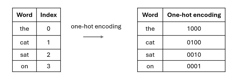
The problem with this simple method is that, as vocabulary grows larger and larger in real-world cases, the one-hot vectors will become extremely long. Also, neural networks are not designed to handle these sparse vectors efficiently.

Additionally, the semantic relationships between related words will be lost during this process as the index for each word is randomly assigned, meaning similar words have no connection in this representation.

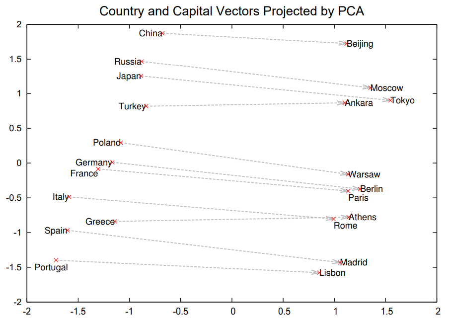
With that, you can better understand the significance of Word2Vec’s contribution now: By representing words as continuous vectors in a high-dimensional space where words with similar contexts have similar vectors, it completely revolutionized the field of NLP.

With Word2Vec, related words will be mapped closer in the embedding space. For example, in the figure below the authors show the PCA projection of word embeddings for some countries and their corresponding capitals, with their relationships automatically captured by Word2Vec without any supervised information provided.

Word2Vec is learnt in an unsupervised manner, and once the embeddings are learnt, they can be easily used in downstream tasks. This is one of the earliest efforts exploring semi-supervised learning in NLP.

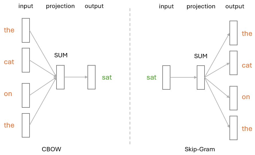
More specifically, it can leverage either the CBOW (Continuous Bag of Words) or Skip-Gram architectures to learn word embeddings.

In CBOW, the model tries to predict the target word based on its surrounding words. For example, given the sentence “The cat sat on the mat,” CBOW would try to predict the target word “sat” given the context words “The,” “cat,” “on,” “the.” This architecture is effective when the goal is to predict a single word from the context.

However, Skip-Gram works quite the opposite way — it uses a target word to predict its surrounding context words. Taking the same sentence as example, this time the target word “sat” becomes the input, and the model would try to predict context words like “The,” “cat,” “on,” and “the.” Skip-Gram is particularly useful for capturing rare words by leveraging the context in which they appear.

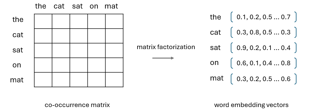
GloVe

Another work along this line of research is GloVe, which is also an unsupervised method to generate word embeddings. Unlike Word2Vec which focuses on a local context, GloVe is designed to capture global statistical information by constructing a word co-occurrence matrix and factorizing it to obtain dense word vectors.

Note that both Word2Vec and GloVe can mainly transfer word-level information, which is often not sufficient in handling complex NLP tasks as we need to capture high-level semantics in the embeddings. This leads to more recent explorations on unsupervised pre-training of NLP models.

Unsupervised Pre-Training

Before GPT, many works have explored unsupervised pre-training with different objectives, such as language model, machine translation and discourse coherence, etc. However, each method only outperforms others on certain downstream tasks and it remained unclear what optimization objectives were most effective or most useful for transfer.

You may have noticed that language models had already been explored as training objectives in some of the earlier works, but why didn’t these methods succeed like GPT?

The answer is Transformer models.

When the earlier works were proposed, there is no Transformer models yet, so researchers could only rely on RNN models like LSTM for pre-training.

This brings us to the next topic: the Transformer architecture used in GPT.

Decoder-only Transformer

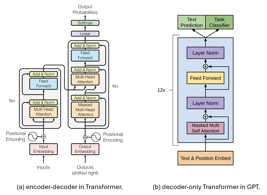
In GPT, the Transformer architecture is a modified version of the original Transformer called decoder-only Transformer. This is a simplified Transformer architecture proposed by Google in 2018, and it contains only the decoder.

Below is a comparison of the encoder-decoder architecture introduced in the original Transformer vs. the decoder-only Transformer architecture used in GPT. Basically, the decoder-only architecture removes the encoder part entirely along with the cross-attention, leading to a more simplified architecture.

So what’s the benefit of making Transformer decoder-only?

Compared with encoder-only models such as BERT, decoder-only models often perform better in generating coherent and contextually relevant text, making them ideal for text generation tasks.

Encoder-only models like BERT, on the other hand, often perform better in tasks that require understanding the input data, like text classification, sentiment analysis, and named entity recognition, etc.

There is another type of models that employ both the encoder and decoder Transformer, such as T5 and BART, with the encoder processes the input, while the decoder generates the output based on the encoded representation. While such a design makes them more versatile in handling a wide range of tasks, they are often more computationally intensive than encoder-only or decoder-only models.

In a nutshell, while both built on Transformer models and tried to leverage pre-training + finetuning scheme, GPT and BERT have chosen very different ways to achieve that similar goal. More specifically, GPT conducts pre-training in an auto-regressive manner, while BERT follows an auto-encoding approach.

Auto-regressive vs. Auto-encoding Language Models

An easy way to understand their difference is to compare their training objectives.

In Auto-regressive language models, the training objective is often to predict the next token in the sequence, based on previous tokens. Due to the dependency on previous tokens, this usually lead to a unidirectional (typically left-to-right) approach, as we show in the left of Figure 6.

By contrast, auto-encoding language models are often trained with objectives like Masked Language Model or reconstructing the entire input from corrupted versions. This is often done in a bi-directional manner where the model can leverage all the tokens around the masked one, in other words, both the left and right side tokens. This is illustrated in the right of Figure 6.

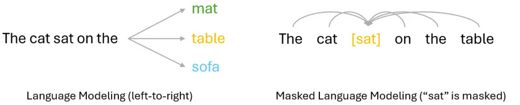
Simply put, auto-regressive LM is more suitable for text generation, but its unidirectional modeling approach may limit its capability in understanding the full context. Auto-encoding LM, on the other hand, can do a better job at context understanding, but is not designed for generative tasks.

Core Concepts in GPT-1

Key Innovations

Most of the key innovations of GPT-1 have already been covered in above sections, so I will just list them here as a brief summary:

• GPT-1 is the first work that successfully leverages auto-regressive language modeling as unsupervised pre-training task, making the pre-training + finetuning paradigm a standard procedure for NLP tasks.
• Unlike its prior works that rely on RNNs and LSTMs, GPT-1 leverages decoder-only Transformer architecture, which improved parallelization and long-range dependency handling, leading to better performance.

Unsupervised Pre-training

In GPT pre-training, a standard language modeling objective is used:

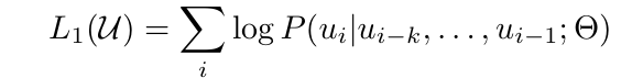
where k is the size of the context window, and the conditional probability P is modeled using the decoder-only Transformer with it parameters represented as θ.

Supervised Finetuning

Once the model is pre-trained, it can be adapted to a specific downstream task by finetuning on a task-specific dataset using a proper supervised learning objective.

One problem here is that GPT requires a continuous sequence of text as input, while some tasks may involve more than one input sequence. For example in Entailment we have both the premise and the hypothesis, and in some QA tasks we will need to handle three different input sequences: the document, the question and the answer.

To make it easier to fit into different tasks, GPT adopts some task-specific input transformations in the finetuning stage, as we show in the figure below:

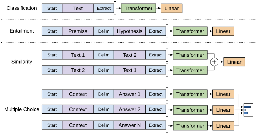
More specifically,

• For Entailment task, the premise and hypothesis sequences will be concatenated into a single sequence, with a delimiter token in between.
• For Similarity task, since there is no inherent ordering of the sentences, we can simply construct two input sequences by switching the two input sequences, get their respective embeddings and then add these two embeddings in a element-wise manner.
• For more complex Question Answering and Commonsense Reasoning tasks, where we are typically given a context document, a question and a set of possible answers, we can concatenate the document context and the question with each possible answer (again with a delimiter token in between), process each of these sequence independently, and then use a softmax layer to produce the final output distribution over possible answers.

Conclusions

In this article, we revisited the key techniques that inspired GPT-1 and highlighted its major innovations.

This is the first part of our GPT series, and in the next article, we will walk through the evolution from GPT-1 to GPT-2, GPT-3, and InstructGPT.

Thanks for reading!

---

Understanding the Evolution of ChatGPT: Part 1—An In-Depth Look at GPT-1 and What Inspired It was originally published in Towards Data Science on Medium, where people are continuing the conversation by highlighting and responding to this story.

Integration architecture focusing on security and access control

1. Introduction

Microsoft Fabric and Azure Databricks are both powerhouses in the data analytics field. These platforms can be used end-to-end in a medallion architecture, from data ingestion to creating data products for end users. Azure Databricks excels in the initial stages due to its strength in processing large datasets and populating the different zones of the lakehouse. Microsoft Fabric performs well in the latter stages when data is consumed. Coming from Power BI, the SaaS setup is easy to use and it provides self-service capabilities to end users.

Given the different strengths of these products and that many customers do not have a greenfield situation, a strategic decision can be to integrate the products. You must then find a logical integration point where both products “meet”. This shall be done with security in mind as this is a top priority for all enterprises.

This blog post first explores three different integration options: Lakehouse split, virtualization with shortcuts, and exposing via SQL API. SQL API is a common integration point between back end and front end and the security architecture of this integration is discussed in more detail in chapter 3. See already the architecture diagram below.

2. Azure Databricks — Microsoft Fabric integration overview

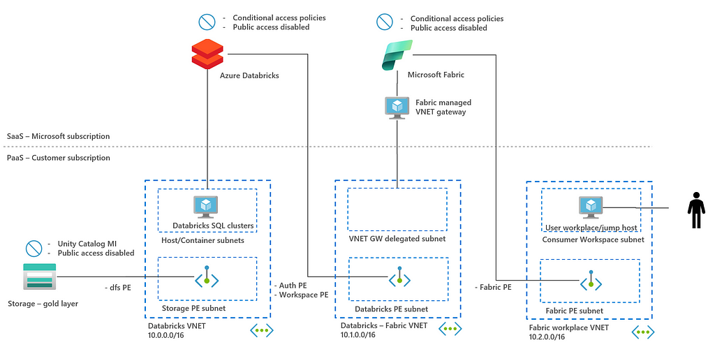
Before diving into the details of securing SQL API architecture, it is helpful to briefly discuss the different options for integrating Azure Databricks and Microsoft Fabric. This chapter outlines three options, highlighting their advantages and disadvantages. For a more extensive overview, refer to this blog.

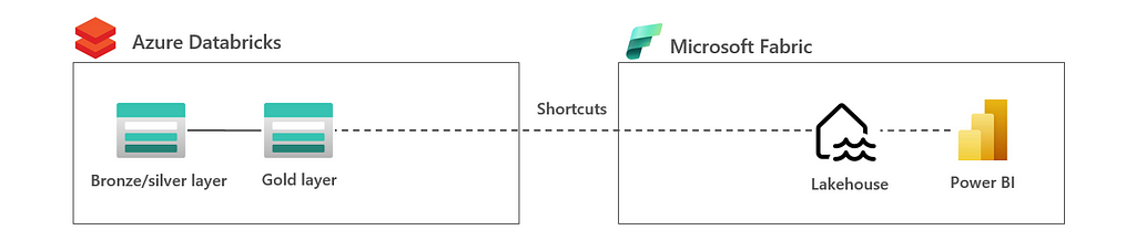
2.1 Lakehouse split: Bronze, silver zone in Databricks | gold zone in Fabric

In this architecture, you can find that data is processed by Databricks up to the silver zone. Fabric copies and processes the data to gold zone in Fabric using V-Ordering. Gold zone data is exposed via a Fabric lakehouse such that data products can be created for end users, see image below.

The advantage of this architecture is that data is optimized for data consumption in Fabric. The disadvantage is that the lakehouse is split over two tools which adds complexity and can give challenges in data governance (Unity Catalog for bronze/silver, but not for gold).

This architecture is most applicable to companies that place a strong emphasis on data analytics in Microsoft Fabric and may even want to eventually migrate the entire lakehouse to Microsoft Fabric.

2.2 Virtualization: Lakehouse in Databricks | shortcuts to Fabric

In this architecture, all data is in the lakehouse is processed by Databricks. Data is virtualized to Microsoft Fabric Lakehouse using ADLSgen2 shortcuts or even a mirrored Azure Databricks Unity Catalog in Fabric, see also the image below.

The advantage of this architecture is that lakehouse is owned by a single tool which gives less challenges in integration and governance. The disadvantage is that data is not optimized for Fabric consumption. In this, you may require additional copies in Fabric to apply V-Ordering, and so optimize for Fabric consumption.

This architecture is most applicable for companies that want to keep the lakehouse Databricks owned and want to enable end users to do analytics in Fabric in which the lack of V-Ordering is not much of a concern. The latter could be true if the data sizes are not too big and/or end users need a data copy anyway.

2.3 Exposing SQL API: Lakehouse in Databricks | SQL API to Fabric

In this architecture, all data is in the lakehouse is processed by Databricks again. However, in this architecture the data is exposed to Fabric using the SQL API. In this, you can decide to use a dedicated Databricks SQL Warehouse or serverless SQL. The main difference with shortcut architecture in the previous bullet, is that data is processed in Databricks rather than Fabric. This can be compared to when a web app fires a SQL query to a database; the query is executed in the database.

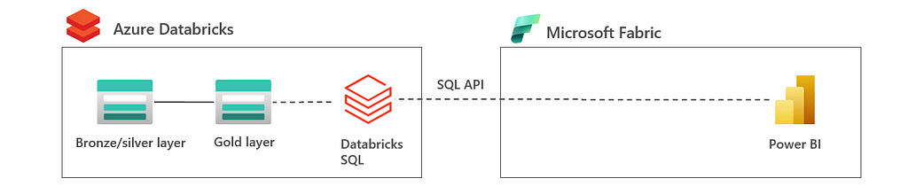
The advantage of this architecture is that lakehouse is owned by a single tool which gives less challenges in integration and governance. Also, SQL API provides a clean interface between Azure Databricks and Microsoft Fabric with less coupling compared to shortcuts. The disadvantage is that end users in Fabric are limited to the Databricks SQL and Fabric is merely used as reporting tool rather than analytics tool.

This architecture is most applicable for companies that want to keep the lakehouse Databricks-owned and are looking to enhance Azure Databricks with the Power BI capabilities that Microsoft Fabric offers.

In the next chapter, a security architecture is discussed for this SQL API integration.

3. Exposing SQL API: security architecture

In this chapter, security architecture is discussed for this SQL API integration. The rationale is that integrating SQL API is a common touch point where back end and front end meet. Furthermore, most security recommendations are applicable for the other architectures discussed earlier.

3.1 Advanced SQL API architecture

To achieve defense in depth, networking isolation and identity-based access control are the two most important steps. You can find this in the diagram below, that was already provided in the introduction of this blog.

In this diagram, three key connectivities that need to be secured are highlighted: ADLSgen2 — Databricks connectivity, Azure Databricks — Microsoft Fabric connectivity and Microsoft Fabric — end user connectivity. In the remaining of this section, the connectivity between the resources is discussed focusing on networking and access control.

In this, it is not in scope to discuss how ADLSgen2, Databricks or Microsoft Fabric can be secured as products themselves. The rationale is that all three resources are major Azure products and offer extensive documentation on how to achieve this. This blog really focuses on the integration points.

3.2 ADLSgen2 — Azure Databricks connectivity

Azure Databricks needs to fetch data from ADLSgen2 with Hierarchical Name Space (HNS) enabled. ADLSgen2 is used as storage since it provides the best disaster recovery capabilities. This includes point-in-time recovery integration with Azure Backup coming in 2025, which offers better protection against malware attacks and accidental deletions. You can find the following networking and access control practices applicable.

Networking: Azure storage public access is disabled. To make sure that Databricks can access the storage account, private endpoints are created in the Databricks VNET. This makes sure that the storage account cannot be accessed from outside the company network and that data stays on the Azure backbone.

Identity-based access control: The storage account can only be accessed via identities and access keys are disabled. To allow Databricks Unity Catalog access to the data, the Databricks access connector identity needs to be granted access using an external location. Depending on the data architecture, this can be an RBAC role to the entire container or a fine-grained ACL/POSIX access rule to the data folder.

3.3 Azure Databricks — Microsoft Fabric connectivity:

Microsoft Fabric needs to fetch data from Azure Databricks. This data shall be used by Fabric to serve end users. In this architecture, the SQL API is used. The networking and identity access control points are also most applicable for the shortcut architecture discussed in paragraph 2.2.

Networking: Azure Databricks public access is disabled. This is both true for the front end as the back end such that clusters are deployed without a public IP address. To make sure that Microsoft Fabric can access data exposed via the SQL API from a network perspective, a data gateway needs to be deployed. It could be decided to deploy a virtual machine in the Databricks VNET, however, that is an IaaS component that needs to be maintained which gives security challenges on its own. A better option is to use a managed virtual network data gateway which is Microsoft managed and provides connectivity.

Identity-based access control: Data in Azure Databricks will be exposed via Unity Catalog. Data in the Unity Catalog shall only be exposed via Identities using fine-grained access control tables and using row-level security. It is not yet possible to use Microsoft Fabric Workspace Identities to access the Databricks SQL API. Instead, a service principal shall be granted access to the data in the Unity Catalog and a personal access token based in this service principal shall be used in the Microsoft Databricks Connector.

3.4 Microsoft Fabric — end user connectivity:

In this architecture, end users will connect to Microsoft Fabric to access reports and to do self-service BI. Within Microsoft, different types of reports can be created based on Power BI. You can apply the following networking and identity-based access controls.

Networking: Microsoft Fabric public access is disabled. Currently, this can only be done at tenant level, as more granular workspace private access will become available in 2025. This can assure that a company can differentiate between private and public workspace. To make sure that end users can access Fabric, private endpoints for Fabric are created in the workspace VNET. This workplace can be peered to the corporate on prem networking using VPN or ExpressRoute. The separation of different networks ensures isolation between the different resources.

Identity-based access control: End users should get access to reports on a need-to-know basis. This can be done to create a separate workspace where reports are stored and to which users get. Also, users shall only be allowed to log in Microsoft Fabric with conditional access policies applied. This way, it can be ensured that users can only log in from hardened devices to prevent data exfiltration.

3.5 Final remarks

In the previous paragraph, an architecture is described where everything is made private and multiple VNET and jumphosts are used. To get your hands dirty and to test this architecture faster, you can decide to test with a simplified architecture below.

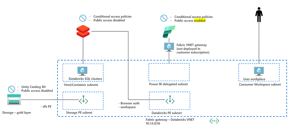
In this architecture, Fabric is configured with public access enabled. Rationale is that Fabric public access setting is currently tenant wide setting. This implies that you need to make all workspaces in a company either private or public. More granular workspace private access will become available in 2025. Also, a single subnet is used to deploy all resources to prevent peering between VNETs and/or deploying multiple jumphosts for connectivity.

4. Conclusion

Microsoft Fabric and Azure Databricks are both powerhouses in the data analytics field. Both tools can cover all parts of the lakehouse architecture, but both tools also have their own strengths. A strategic decision could be to integrate the tools especially if there is a non green situation and both tools are used in a company.

Three different architectures to integrate are discussed: Lakehouse split, virtualization with shortcuts and exposing via SQL API. The first two architectures are more relevant in case you want to put more emphasize on the Fabric analytics capabilities, whereas the last SQL API architecture is more relevant if you want to focus on the Fabric Power BI reporting capabilities.

In the remainder of the blog, a security architecture is provided for the SQL API architecture in which there is a focus on network isolation, private endpoints and identity. Although this architecture focuses on exposing data from the Databricks SQL, the security principles are also applicable for the other architectures.

In short: There are numerous things to take into account if and where to integrate Azure Databricks with Microsoft Fabric. However, this shall always be done with security in mind. This blog aimed to give you an in-depth overview using the SQL API as practical example.

---

How to Securely Connect Microsoft Fabric to Azure Databricks SQL API was originally published in Towards Data Science on Medium, where people are continuing the conversation by highlighting and responding to this story.