Provide an LLM agent with a suite of robust tools it can use to interact with a graph database
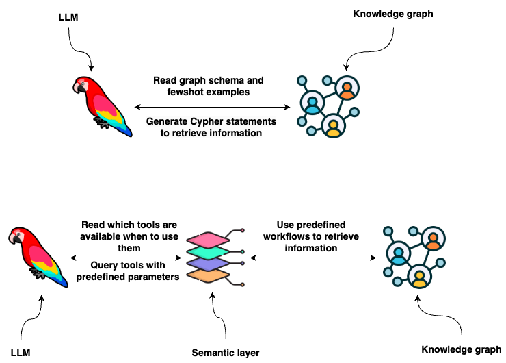
Knowledge graphs provide a great representation of data with flexible data schema that can store structured and unstructured information. You can use Cypher statements to retrieve information from a graph database like Neo4j. One option is to use LLMs to generate Cypher statements. While that option provides excellent flexibility, the truth is that base LLMs are still brittle at consistently generating precise Cypher statements. Therefore, we need to look for an alternative to guarantee consistency and robustness. What if, instead of developing Cypher statements, the LLM extracts parameters from user input and uses predefined functions or Cypher templates based on the user intent? In short, you could provide the LLM with a set of predefined tools and instructions on when and how to use them based on the user input, which is also known as the semantic layer.
Semantic layer is an intermediate step that provides additional accuracy and robust way of LLMs interacting with a Knowledge graph. Image by the author. Inspired by this image.
A semantic layer consists of various tools exposed to an LLM that it can use to interact with a knowledge graph. They can be of various complexity. You can think of each tool in a semantic layer as a function. For example, take a look at the following function.
def get_information(entity: str, type: str) -> str:
    candidates = get_candidates(entity, type)
    if not candidates:
        return "No information was found about the movie or person in the database"
    elif len(candidates) > 1:
        newline = "n"
        return (
            "Need additional information, which of these "
            f"did you mean: {newline + newline.join(str(d) for d in candidates)}"
        )
    data = graph.query(
        description_query, params={"candidate": candidates[0]["candidate"]}
    )
    return data[0]["context"]
The tools can have multiple input parameters, like in the above example, which allows you to implement complex tools. Additionally, the workflow can consist of more than a database query, allowing you to handle any edge cases or exceptions as you see fit. The advantage is that you turn prompt engineering problems, which might work most of the time, into code engineering problems, which work every time exactly as scripted.
Movie agent
In this blog post, we will demonstrate how to implement a semantic layer that allows an LLM agent to interact with a knowledge graph that contains information about actors, movies, and their ratings.
Movie agent architecture. Image by the author.
Taken from the documentation (also written by me):
The agent utilizes several tools to interact with the Neo4j graph database effectively.
* Information tool: Retrieves data about movies or individuals, ensuring the agent has access to the latest and most relevant information.
* Recommendation Tool: Provides movie recommendations based upon user preferences and input.
* Memory Tool: Stores information about user preferences in the knowledge graph, allowing for a personalized experience over multiple interactions.
An agent can use information or recommendation tools to retrieve information from the database or use the memory tool to store user preferences in the database. Predefined functions and tools empower the agent to orchestrate intricate user experiences, guiding individuals towards specific goals or delivering tailored information that aligns with their current position within the user journey. This predefined approach enhances the robustness of the system by reducing the artistic freedom of an LLM, ensuring that responses are more structured and aligned with predetermined user flows, thereby improving the overall user experience.
The semantic layer backend of a movie agent is implemented and available as a LangChain template. I have used this template to build a simple streamlit chat application.
Streamlit chat interface. Image by the author.
Code is available on GitHub. You can start the project by defining environment variables and executing the following command:
docker-compose up
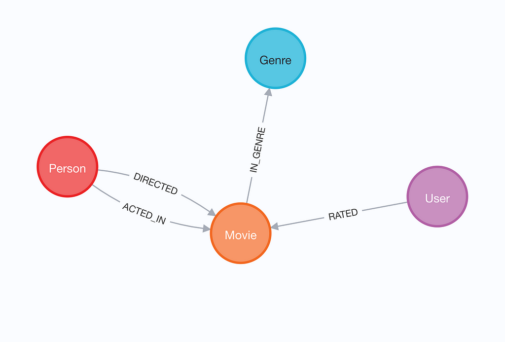
Graph model
The graph is based on the MovieLens dataset. It contains information about actors, movies, and 100k user ratings of movies.
Graph schema. Image by the author.
The visualization depicts a knowledge graph of individuals who have either acted in or directed a movie, which is further categorized by genre. Each movie node holds information about its release date, title, and IMDb rating. The graph also contains user ratings, which we can use to provide recommendations.
You can populate the graph by executing the ingest.py script, which is located in the root directory of the folder.
Defining tools
Now, we will define the tools an agent can use to interact with the knowledge graph. We will start with the information tool. Information tool is designed to fetch relevant information about actors, directors, and movies. The Python code looks the following:
def get_information(entity: str, type: str) -> str:
    # Use full text index to find relevant movies or people
    candidates = get_candidates(entity, type)
    if not candidates:
        return "No information was found about the movie or person in the database"
    elif len(candidates) > 1:
        newline = "n"
        return (
            "Need additional information, which of these "
            f"did you mean: {newline + newline.join(str(d) for d in candidates)}"
        )
    data = graph.query(
        description_query, params={"candidate": candidates[0]["candidate"]}
    )
    return data[0]["context"]
The function starts by finding relevant people or movies mentioned using a full-text index. The full-text index in Neo4j uses Lucene under the hood. It enables a seamless implementation of text distance-based lookups, which allow the user to misspell some words and still get results. The function starts by finding relevant people or movies mentioned using a full-text index. The full-text index in Neo4j uses Lucene under the hood. It enables a seamless implementation of text distance-based lookups, which allow the user to misspell some words and still get results. If no relevant entities are found, we can directly return a response. On the other hand, if multiple candidates are identified, we can guide the agent to ask the user a follow-up question and be more specific about the movie or person they are interested in. Imagine that a user asks, “Who is John?”.
print(get_information("John", "person"))
# Need additional information, which of these did you mean:
# {'candidate': 'John Lodge', 'label': 'Person'}
# {'candidate': 'John Warren', 'label': 'Person'}
# {'candidate': 'John Gray', 'label': 'Person'}
In this case, the tool informs the agent that it needs additional information. With simple prompt engineering, we can steer the agent to ask the user a follow-up question. Suppose the user is specific enough, which allows the tool to identify a particular movie or a person. In that case, we use a parametrized Cypher statement to retrieve relevant information.
print(get_information("Keanu Reeves", "person"))
# type:Actor
# title: Keanu Reeves
# year:
# ACTED_IN: Matrix Reloaded, The, Side by Side, Matrix Revolutions, The, Sweet November, Replacements, The, Hardball, Matrix, The, Constantine, Bill & Ted's Bogus Journey, Street Kings, Lake House, The, Chain Reaction, Walk in the Clouds, A, Little Buddha, Bill & Ted's Excellent Adventure, The Devil's Advocate, Johnny Mnemonic, Speed, Feeling Minnesota, The Neon Demon, 47 Ronin, Henry's Crime, Day the Earth Stood Still, The, John Wick, River's Edge, Man of Tai Chi, Dracula (Bram Stoker's Dracula), Point Break, My Own Private Idaho, Scanner Darkly, A, Something's Gotta Give, Watcher, The, Gift, The
# DIRECTED: Man of Tai Chi
With this information, the agent can answer most of the questions that concern Keanu Reeves.
Now, let’s guide the agent on utilizing this tool effectively. Fortunately, with LangChain, the process is straightforward and efficient. First, we define the input parameters of the function using a Pydantic object.
class InformationInput(BaseModel):
    entity: str = Field(description="movie or a person mentioned in the question")
    entity_type: str = Field(
        description="type of the entity. Available options are 'movie' or 'person'"
    )
Here, we describe that both entity and entity_type parameters are strings. The entity parameter input is defined as the movie or a person mentioned in the question. On the other hand, with the entity_type, we also provide available options. When dealing with low cardinalities, meaning when there is a small number of distinct values, we can provide available options directly to an LLM so that it can use valid inputs. As we saw before, we use a full-text index to disambiguate movies or people as there are too many values to provide directly in the prompt.
Now let’s put it all together in a Information tool definition.
class InformationTool(BaseTool): name = "Information" description = ( "useful for when you need to answer questions about various actors or movies" ) args_schema: Type[BaseModel] = InformationInput
Accurate and concise tool definitions are an important part of a semantic layer, so that an agent can correctly pick relevant tools when needed.
The recommendation tool is slightly more complex.
def recommend_movie(movie: Optional[str] = None, genre: Optional[str] = None) -> str:
    """
    Recommends movies based on user's history and preference
    for a specific movie and/or genre.
    Returns:
        str: A string containing a list of recommended movies, or an error message.
    """
    user_id = get_user_id()
    params = {"user_id": user_id, "genre": genre}
    if not movie and not genre:
        # Try to recommend a movie based on the information in the db
        response = graph.query(recommendation_query_db_history, params)
        try:
            return ", ".join([el["movie"] for el in response])
        except Exception:
            return "Can you tell us about some of the movies you liked?"
    if not movie and genre:
        # Recommend top voted movies in the genre the user haven't seen before
        response = graph.query(recommendation_query_genre, params)
        try:
            return ", ".join([el["movie"] for el in response])
        except Exception:
            return "Something went wrong"

    candidates = get_candidates(movie, "movie")
    if not candidates:
        return "The movie you mentioned wasn't found in the database"
    params["movieTitles"] = [el["candidate"] for el in candidates]
    query = recommendation_query_movie(bool(genre))
    response = graph.query(query, params)
    try:
        return ", ".join([el["movie"] for el in response])
    except Exception:
        return "Something went wrong"
The first thing to notice is that both input parameters are optional. Therefore, we need to introduce workflows that handle all the possible combinations of input parameters and the lack of them. To produce personalized recommendations, we first get a user_id , which is then passed into downstream Cypher recommendation statements.
Similarly as before, we need to present the input of the function to the agent.
class RecommenderInput(BaseModel):
    movie: Optional[str] = Field(description="movie used for recommendation")
    genre: Optional[str] = Field(
        description=(
            "genre used for recommendation. Available options are:" f"{all_genres}"
        )
    )
Since only 20 available genres exist, we provide their values as part of the prompt. For movie disambiguation, we again use a full-text index within the function. As before, we finish with the tool definition to inform the LLM when to use it.
class RecommenderTool(BaseTool): name = "Recommender" description = "useful for when you need to recommend a movie" args_schema: Type[BaseModel] = RecommenderInput
So far, we have defined two tools to retrieve data from the database. However, the information flow doesn’t have to be one-way. For example, when a user informs the agent they have already watched a movie and maybe liked it, we can store that information in the database and use it in further recommendations. Here is where the memory tool comes in handy.
def store_movie_rating(movie: str, rating: int):
    user_id = get_user_id()
    candidates = get_candidates(movie, "movie")
    if not candidates:
        return "This movie is not in our database"
    response = graph.query(
        store_rating_query,
        params={"user_id": user_id, "candidates": candidates, "rating": rating},
    )
    try:
        return response[0]["response"]
    except Exception as e:
        print(e)
        return "Something went wrong"


class MemoryInput(BaseModel):
    movie: str = Field(description="movie the user liked")
    rating: int = Field(
        description=(
            "Rating from 1 to 5, where one represents heavy dislike "
            "and 5 represent the user loved the movie"
        )
    )
The memory tool has two mandatory input parameters that define the movie and its rating. It’s a straightforward tool. One thing I should mention is that I noticed in my testing that it probably makes sense to provide examples of when to give a specific rating, as the LLM isn’t the best at it out of the box.
llm_with_tools = llm.bind(functions=[format_tool_to_openai_function(t) for t in tools])
prompt = ChatPromptTemplate.from_messages( [ ( "system", "You are a helpful assistant that finds information about movies " " and recommends them. If tools require follow up questions, " "make sure to ask the user for clarification. Make sure to include any " "available options that need to be clarified in the follow up questions " "Do only the things the user specifically requested. ", ), MessagesPlaceholder(variable_name="chat_history"), ("user", "{input}"), MessagesPlaceholder(variable_name="agent_scratchpad"), ] )
LangChain expression language makes it very convenient to define an agent and expose all its functionalities. We won’t go into LCEL syntax as that is beyond the scope of this blog post.
The movie agent backend is exposed as an API endpoint using LangServe.
Streamlit chat application
Now we just have to implement a streamlit application that connects to the LangServe API endpoint and we are good to go. We’ll just look at the async function that is used to retrieve an agent response.
async def get_agent_response(
    input: str, stream_handler: StreamHandler, chat_history: Optional[List[Tuple]] = []
):
    url = "http://api:8080/movie-agent/"
    st.session_state["generated"].append("")
    remote_runnable = RemoteRunnable(url)
    async for chunk in remote_runnable.astream_log(
        {"input": input, "chat_history": chat_history}
    ):
        log_entry = chunk.ops[0]
        value = log_entry.get("value")
        if isinstance(value, dict) and isinstance(value.get("steps"), list):
            for step in value.get("steps"):
                stream_handler.new_status(step["action"].log.strip("n"))
        elif isinstance(value, str):
            st.session_state["generated"][-1] += value
            stream_handler.new_token(value)
The function get_agent_response is designed to interact with a movie-agent API. It sends a request with the user’s input and chat history to the API and then processes the response asynchronously. The function handles different types of responses, updating the stream handler with new statuses and appending the generated text to the session state, which allows us to stream results to the user.
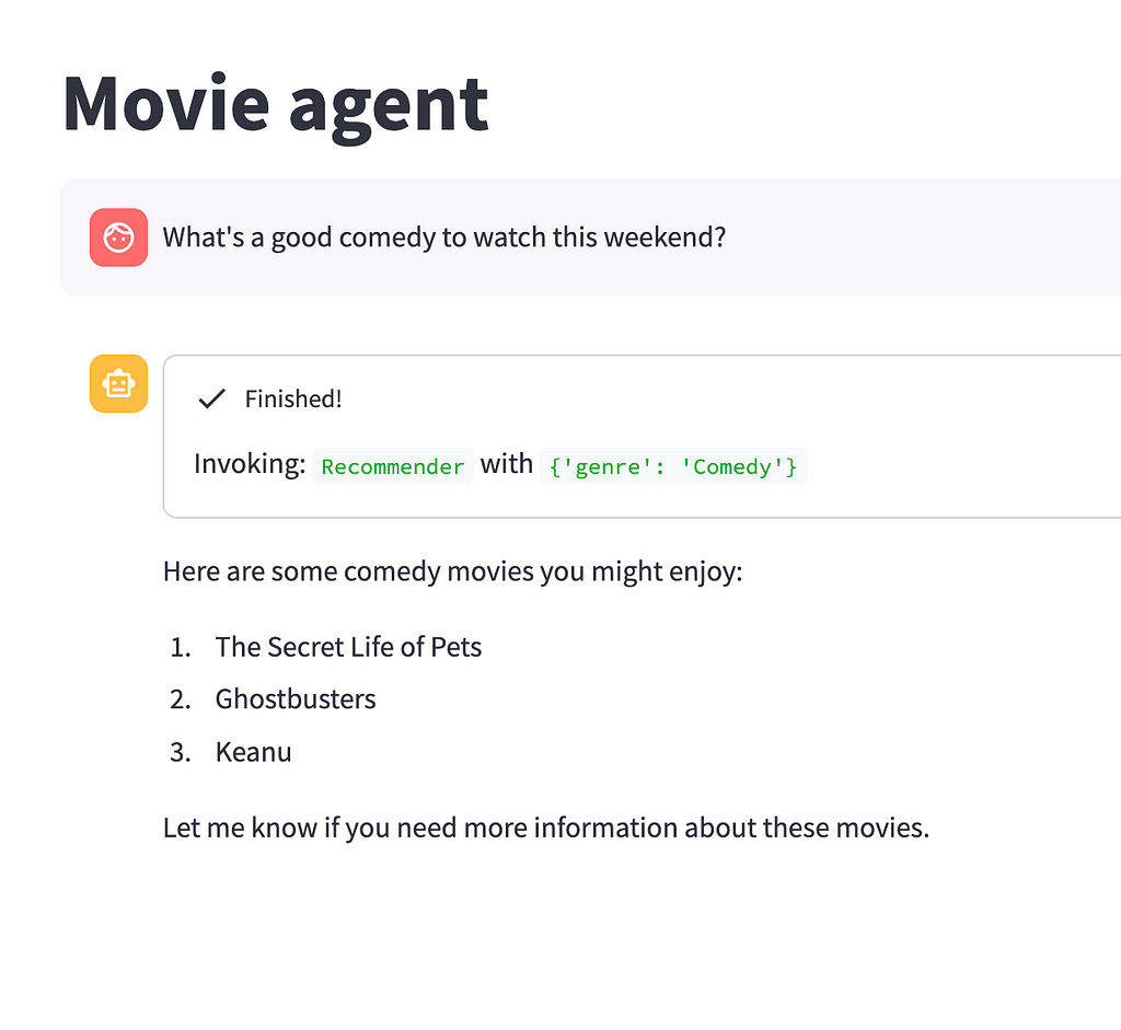
Let’s now test it out
Movie agent in action. Image by the author.
The resulting movie agent offers a surprisingly good and guided interaction with the user.
Conclusion
In conclusion, the integration of a semantic layer in language model interactions with graph databases, as exemplified by our Movie Agent, represents a significant leap forward in enhancing user experience and data interaction efficiency. By shifting the focus from generating arbitrary Cypher statements to utilizing a structured, predefined suite of tools and functions, the semantic layer brings a new level of precision and consistency to language model engagements. This approach not only streamlines the process of extracting relevant information from knowledge graphs but also ensures a more goal-oriented, user-centric experience.
The semantic layer acts as a bridge, translating user intent into specific, actionable queries that the language model can execute with accuracy and reliability. As a result, users benefit from a system that not only understands their queries more effectively but also guides them towards their desired outcomes with greater ease and less ambiguity. Furthermore, by constraining the language model’s responses within the parameters of these predefined tools, we mitigate the risks of incorrect or irrelevant outputs, thereby enhancing the trustworthiness and reliability of the system.
F. Maxwell Harper and Joseph A. Konstan. 2015. The MovieLens Datasets: History and Context. ACM Transactions on Interactive Intelligent Systems (TiiS) 5, 4: 19:1–19:19. https://doi.org/10.1145/2827872
Many complex networks evolve over time including transaction networks, traffic networks, social networks and more. Temporal Graph Learning (TGL) is a fast growing field which aims to learn, predict and understand evolving networks. See our previous blog post for an introduction to temporal graph learning and a summary of advancements last year.
In 2023, we saw significantly increased interest from both academia and the industry in the development of TGL. Compared to last year, the number of submissions at the temporal graph learning workshop @ NeurIPS 2023 tripled, resulting in 35 accepted papers. In addition, the temporal graph learning reading group, started in February 2023, has now hosted 28 research talks (find the recordings on YouTube). With nearly 200 researchers signed up for the reading group, we are glad to see witness interest in the topic and an extremely active community.
This blog post covers a selection of exciting developments in TGL while pointing out research directions for 2024. We also ask leading researchers for their take on what the future holds for TGL. This blog also aims to provide references and act as starting points for those who want to learn more about temporal graph learning. Please share with us in the comment section any other advances you are excited about.
One of the driving forces of the rapid development of machine learning on graphs is the availability of standardized and diverse benchmarks such as the Open Graph Benchmark (OGB), the Long Range Graph Benchmark and GraphWorld. However, these benchmarks are designed for static graphs and lack the fine-grained timestamp information required for temporal graph learning. Therefore, progress in temporal graph learning has been held back by the lack of large high-quality datasets, as well as the lack of proper evaluation resulting in over-optimistic performances.
To address this gap, the Temporal Graph Benchmark (TGB) was presented recently, including a collection of challenging and diverse benchmark datasets for realistic, reproducible, and robust evaluation for machine learning on temporal graphs. TGB provides a pypi package to automatically download and process nine datasets from five distinct domains with up to 72 million edges and 30 million timestamps. TGB also provides standardized evaluation motivated by real applications.
TGB: Challenging and Realistic Benchmark for Temporal Graph Learning. Image source: Huang et al. 2023, by authors.
TGB includes both link and node level tasks and an extensive empirical comparison of state-of-the-art TG models on all datasets. The first task is the dynamic link property prediction task which predicts the property (often existence) of a link between a pair of nodes at a future time. In TGB, this task is modeled as a ranking problem and evaluated with the filtered Mean Reciprocal Rank (MRR) metric. Results show that model rankings vary significantly across datasets with different ratios of test set edges which are never observed during training. In addition, model performance deteriorates as more negative samples (non-existence edges) are used in the evaluation. Interestingly, the extent of performance drop varies across models as well.
In the dynamic node property prediction task, the goal is to predict the property of a node at a given time. More specifically we focus on the node affinity prediction task which models how the user preference towards different items shift over time. Here, we use the Normalized Discounted Cumulative Gain of the top 10 items (NDCG@10) to compare the relative order of the predicted items to that of the ground truth. Interesting, we found that single heuristics outperform existing TG models and this highlights the need for more models focusing on node level tasks in the future. The TGB leaderboard is public and you are welcome to submit your model via a google form. For more details, see the TGB blog post by the authors of this blog.
Novel Architectures for Link Prediction
“Link prediction in the realm of temporal graph learning poses a significant challenge. The learning algorithms must extend beyond the limited expressive power typically found in traditional message passing architectures like GNNs. Additionally, they must emphasize computational efficiency. A critical aspect of this is ensuring low latency in responding to link prediction queries, striking a balance between the expressive power of the model and the speed of its predictions in a dynamic and complex data environment.” — Pan Li, Assistant Professor, Georgia Institute of Technology
A recent survey by Longa et al. provides a comprehensive overview of temporal GNNs. Many approaches proposed specialized architectures for dynamic link prediction, often aiming to capture important structure properties or correlations. For example, Luo et al. aimed to explicitly model the joint neighborhood of a set of nodes for future link prediction where they designed the Neighborhood-Aware Temporal network model (NAT). The joint neighborhood is not captured by traditional Graph Neural Network (GNN) based approaches as the node embedding vectors are generated independently for each node. In the following example, node v and w have the same structural contexts thus indistinguishable in the eyes of GNNs. In reality, the link between node u and v at t₃ is more likely to form due to the triadic closure law while this is not sure for the link between u and w at t₃. In comparison, NAT adapted a novel dictionary-type neighborhood representation which records k-hop neighborhood information and allows fast construction of structure features of joint neighborhood of multiple nodes. The dictionary representation is maintained by an efficient cache technique named N-cache. N-caches allowed NAT to construct the joint neighborhood features for a batch of node pairs for fast link prediction.
GNN embeddings of node v and w would be identical. Image source: Luo et al. 2022
Second, Yu et al. aim to capture long-term temporal dependencies by proposing DyGFormer, a new Transformer-based architecture for temporal graph learning. Given a query between node u and node v at time t, the first step is to extract historical first-hop interactions of node u and v before time t. This includes the encodings of neighbors, links, time intervals as well as the frequencies of every neighbor’s appearances of u and v. The assumption is that if u and v share more common historical neighbors in the past, then they are more likely to interact in the future. After encoding the historical interactions in a sequence, it is then divided into multiple patches and fed into a transformer for capturing temporal dependencies.
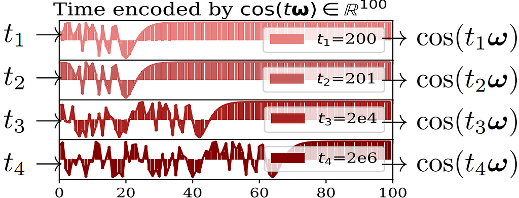
Another question is do we really need complicated model architectures for temporal networks? In a paper with the same name, Cong et al. examined the necessity of common modules used in temporal graph learning such as Recurrent Neural Network (RNN) and the self-attention mechanism. They showed that these modules are not always necessary for dynamic link prediction. In particular, their proposed GraphMixer model is based entirely on multi-layer perceptrons (MLPs) and neighbor mean-pooling while performing strongly against baselines with RNN and self-attention. GraphMixer contains three modules: a link-encoder summarizes the information from temporal links, a node-encoder extracts information from nodes and a link-classifier which combines the above information for prediction. Interestingly, Cong et al. argued that a trainable time-encoding function could cause instability during training and instead opted for a fixed time-encoding function z(t) = cos(tω) where fixed features capture the relative difference between two timestamps as shown below.
Fixed time encoding function to convert t into a vector cos(tω). x-axis is the vector dimension and y-axis is the cosine value. Image source: Cong et al. 2023
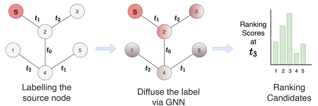
Lastly, Suresh et al. pointed out that existing methods maximizes accuracy independently over future links, ignoring the fact that future links often have dependency between each other. This is seen when a user selects among a list of items to purchase or a set of users to connect in a social network. Therefore, Suresh et al. treat dynamic link prediction as a ranking problem and propose Temporal Graph network for RANKing (TGRank) to learn to rank over a list of candidates. The pipeline of TGRank is shown below. The task query now contains a center node s (in the example) with a set of candidate nodes (all other nodes in the subgraph) and the goal is to rank the most likely candidate as the destination of node s. To this end, TGRank follows three steps. First, the node s is labeled differently from other nodes. Then, GNNs are used to diffuse the center node label to every ranking candidate. This parametrized label diffusion step aggregates timestamps, multiplicity as well as features of historical interactions along the network from the center node to all candidates and provides provably more expressive power for link prediction. Lastly, a list-wise loss is used to optimize the ranking amongst candidates jointly. Empirically, it is also shown that with a listwise ranking loss, popular models such as TGN and TGAT also perform better than their original setup with binary classification loss.
Pipeline of TGRank. The center node is node s. Image source: Suresh et al. 2023
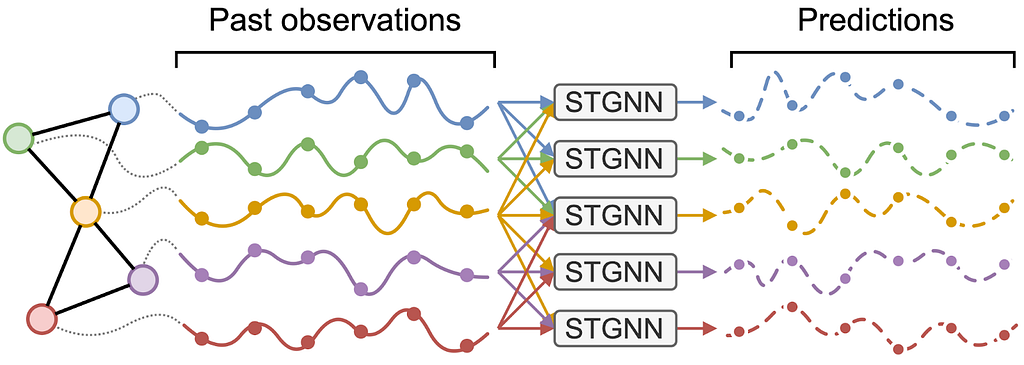
Spatiotemporal Graphs and Graph Deep Learning for Time Series Processing
“Basing our predictions primarily on the most related observations is sensible, yet not always straightforward, as relevant data relations often hide in plain sight. Unveiling them is a captivating challenge, particularly when they are dynamic or involve more than two entities.” — Daniele Zambon, PostDoc at The Swiss AI Lab IDSIA
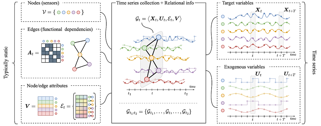
In the temporal graph learning community, the term spatiotemporal graph has been often used to indicate a graph with fixed topology and node features that change over time, usually at discrete time steps corresponding to regularly sampled observations. More recently the problem of processing data with such a structure is being considered from a different perspective, i.e., by considering the dynamic node feature as time series and edges as functional dependencies among sequences of observations (Cini et al. 2023, Ming et al. 2023). From this perspective, which significantly deviates from many of the settings discussed elsewhere in this blog post, spatiotemporal graph-based representations allow for processing collections of correlated time series by taking advantage of the architectural biases typical of graph neural networks.
Correlated time series with relational side information Image source: Cini et al. 2023, by authors.
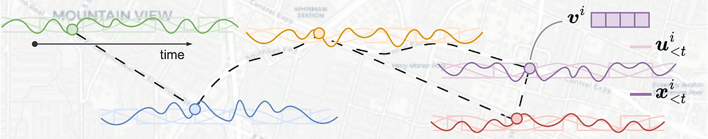
Such sets of correlated time series can be generated by sensors, either physical or not. An example is in the traffic domain, where time series might correspond to readings of sensors measuring the number of vehicles passing by at a crossroads. Each sensor will correspond to a different node and an adjacency matrix can be obtained, for instance, by joining with an edge only those sensors directly connected by a road segment. Besides traffic forecasting (Li et al. 2018, Yu et al. 2018), these representations have been used in a wide range of time series processing applications ranging from air quality monitoring (Chen et al. 2021) and energy analytics (Cini et al. 2023) to biomedical data processing (Zhang et al. 2022) and financial time series analysis (Matsunaga et al. 2019).
Example of correlated time series from the traffic domain. Image source: tutorial at ECML PKDD 2023 by authors.
To process this data, the standard message-passing framework needs to be updated to handle sequences of observations coming from the neighborhood of each node. This can easily be done by replacing the proper operators (i.e., the message and update functions) with operators able to process the data along the temporal dimension, e.g., recurrent cells (Seo et al. 2018), spatiotemporal convolutions (Wu et al. 2019) and attention-based architectures (Marisca et al. 2022). The resulting models are known as spatiotemporal graph neural networks (STGNNs) and there has been a large amount of research dedicated to coming up with effective architectures (see Ming et al. 2023). One of the main advantages of using STGNNs is that the same set of parameters can be used to forecast any subset of time series, while taking dependencies into account throughout the processing. This is a massive advantage over standard multivariate time series forecasting models that usually would have to forecast each time series separately or give up parameter sharing. Hybrid STGNNs, with some time-series-specific parameters, can also be considered and, as we have shown in a recent NeurIPS paper, often outperform models where all parameters are shared. Besides the model architecture, graph-based representations, as shown by Zambon et al., can also help in assessing the optimality of a forecasting model by focusing the spatiotemporal correlation analysis to interconnected nodes.
A spatiotemporal graph neural network. Image by authors.
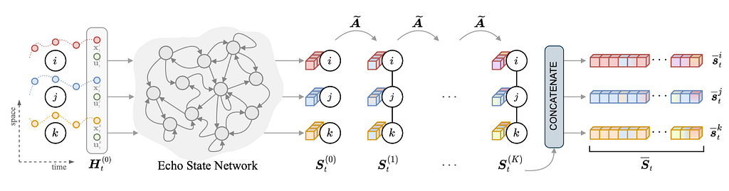
Several challenges are inherent to the field, starting from dealing with irregularly sampled time series and missing data; indeed, both are quite common phenomena when dealing with actual cyber-physical systems. Luckily, graph-based models are useful in this context as well, for example allowing to condition the reconstruction on observations at neighboring sensors. Scalability is another major concern as differently from standard GNNs, message-passing is often performed w.r.t. each time step. Existing scalable architectures mostly rely on subsampling and/or pre-computed node features. When no prior relation information is available, the challenge becomes that of learning a latent graph directly from the time series. The problem has been tackled, for example, by directly learning an adjacency matric (e.g., Wu et al. 2019) or, under a probabilistic framework, by relying on reparametrization tricks and score-based estimators.
A scalable spatiotemporal graph neural network Image source: Cini et al. 2023. by authors
Since this topic was not covered in last year’s blog post, the objective here was to give a short overview of the settings and the problems that can be modeled. Many directions are currently being explored, from graph state-space models and graph Kalman filters to diffusion-based and continuous space-time models. If you are interested in knowing more and/or using these models in practice, we recently released a comprehensive tutorial paper on the topic. You can also check out Torch Spatiotemporal (tsl), our library to build graph-based time series processing pipelines.
There were surprisingly few temporal KG papers in this year’s top ML conferences: TILP (Xiong et al. 2023) on deriving temporal rule learning competitive with neural methods, and theory work by Chen and Wang to measure expressiveness of temporal GNNs. In fact, the most interesting (to me) papers on this topic were found at the TGL workshop at NeurIPS’23 (one more reason for you to follow the venue!), e.g., predicting future time intervals by Pop and Kostylev, or identifying leakages in standard benchmarking datasets by Pan et al. Finally, I’d outline the Unified Urban KG (UUKG) by Ning et al as a fresh look on temporal KG datasets that actually make practical sense and a use-case — modeling transportation flows in the city.
UUKG illustrates the biggest problem of the shrinking temporal KG community — the lack of practically important tasks and datasets where it would be possible to demonstrate the utility of the data modeling paradigm in real-world tasks. That is, adding 1% of MRR/Hits@10 on 10-year old KG embedding benchmarks is rather useless these days compared to the successes of Geometric Deep Learning in biology or materials science (or compared to LLMs, but that’s a story for another day). Hopefully, we will see more UUKG-like practically useful datasets.
Perhaps another adjacent area where temporal KGs might make a difference is heterogeneous graphs (that usually have typed edges) that are much more used in industry. For example, the recent RelBench (Relational Deep Learning Benchmark) formulates a temporal prediction problem over relational databases that can be easily converted to KGs or hypergraphs.
Causality-Aware Temporal Graph Learning
“Einstein said the arrow of time flies in only one direction. […] And who among us, offered the chance, would not relive the day or hour in which we first knew love, or ecstasy, or made a choice that forever altered our future, negating a life we might have had? Such chances are rarely granted.” — Greg Iles, The Quiet Game
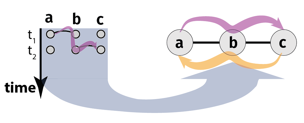
One reason why temporal graph learning is interesting is that — depending on the data at hand — it requires different perspectives. As an example, consider temporal graphs data with high-resolution (possibly continuous) time stamps. In such data, discrete-time graph learning techniques that utilize sequences of snapshot graphs require a coarse-graining of time, where each snapshot consists of edges occurring in a certain time interval. This coarse-graining allows to generalize (static) graph learning techniques to time series data. But it introduces a major issue: Each snapshots discards information on the temporal order in which edges occurred, which is the foundation of causal or time-respecting paths (Kempe et al. 2000). Like paths in static graphs, time-respecting paths are important since they tell us which nodes can causally influence each other indirectly. Below, we illustrate this in a simple temporal graph with two undirected edges (a,b) and (b,c) occurring at times t₁ and t₂ respectively. If (a,b) occurs before (b,c), a can causally influence c via a time-respecting path (indicated in purple) passing through b. If the temporal order of edges is reversed, a cannot causally influence c, since any influence must propagate backwards in time. Note that the directedness of the influence from a to c is due to the directed arrow of time and despite the fact that both edges are undirected. Moreover, while two edges (a,b) and (b,c) in a static, time-aggregated graph imply a transitive path from a via b to c (purple) and vice-versa (orange), this is not true for temporal graphs.
Time-respecting path from node a to node c. Image by authors.
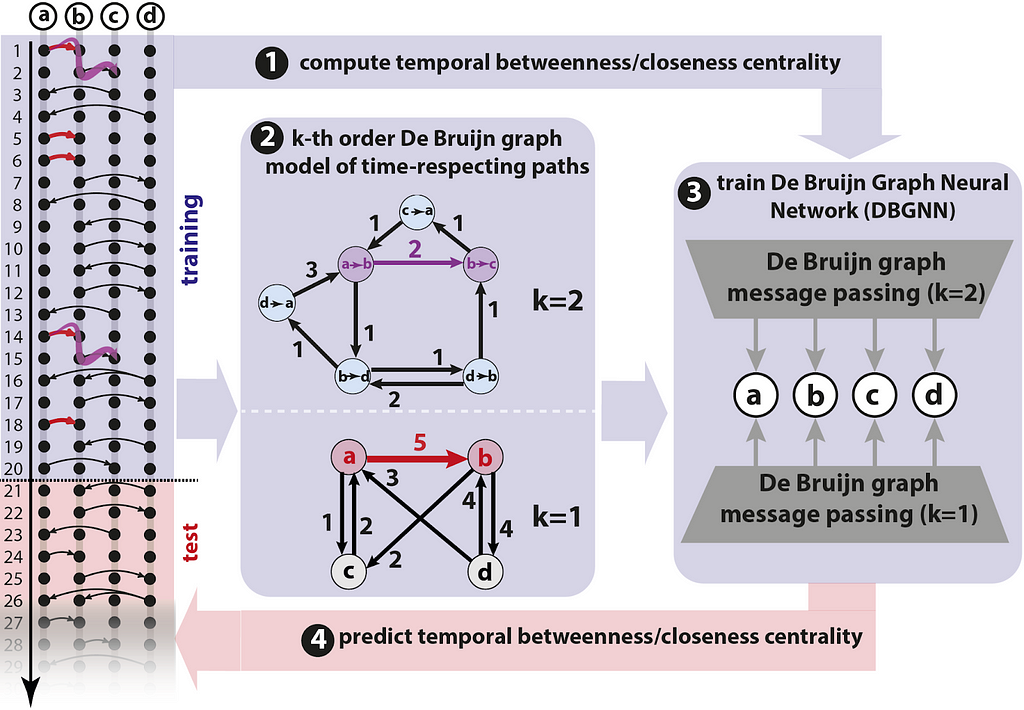
Several works have shown that — due to the arrow of time — the causal topologyof temporal graphs, i.e. which nodes can possibly causally influence each other via time-respecting paths, strongly differs from their static counterparts, with interesting implications for epidemic spreading (Pfitzner et al. 2013), diffusion speed (Scholtes et al. 2014), node centralities (Rosvall et al. 2014), or community detection (Lambiotte et al. 2019). Can we make deep learning methods aware of patterns in the causal topology of temporal graphs? Advances presented at this year show that this can be achieved based on models that generalize commonly used static representations of temporal graphs. Consider a weighted time-aggregated graph, where a (directed) edge (a,b) with weight five captures that (a,b) occurred five times in a temporal graph. Such a weighted, time-aggregated graph is illustrated in the bottom of panel 2 in the figure below.
Pipeline to predict temporal centralities of nodes in a temporal graph. Image source: Heeg et al., by authors
Each edge in the temporal graph is a time-respecting path with length one. A weighted time-aggregated graph thus corresponds to a first-order model for the causal topology of a temporal graph, which captures time-respecting paths of length one. It neglects the temporal ordering of edges, since we only count how often each edge occurred. A line graph transformation enables us to generalize this idea tocausality-aware modelsthat facilitate temporal graph learning: We simply replace edges in the first-order graph by nodes in a second-order graph, i.e. we turn edges (a,b) and (b,c) into nodes “a→b” and “b→c”, respectively. In the resulting second-order graph (see the top graph in panel 2 in figure), we can use edges to represent time-respecting paths of length two, i.e. edge (a→b, b→c) indicates that a causally influence c via b. However, the reverse order of edges are not included. If the edges occur in reverse order, we do not include (a→b, b→c). Importantly, such a second-order graph is sensitive to the temporal ordering of edges, while a first-order graph is not! In Scholtes, 2017, this is generalized to higher orders, which yields k-th order De Bruijn graph models for the causal topology oftemporal graphs.
Qarkaxhija et al. have shown that neural message passing in such higher-order De Bruijn graphs yields a causality-aware graph neural network architecture for temporal graphs. Building on these De Bruijn Graph Neural Networks (DBGNN), in a poster at this year’s TGL workshop, Heeg and Scholtes address the challenge to predict temporal betweenness and closeness centralities of nodes. Since they are influenced by the arrow of time, temporal node centralities can drastically differ from static centralities. Moreover, it is costly to compute them! This is addressed by training a DBGNN model on a first time interval of a temporal graph, then using the trained model to forecast temporal centralities in the remaining data. The overall approach is illustrated above. Empirically results are promising and showcased the potential of causality-aware graph learning. We also hope to see more attention from the community in learning causal structure on temporal graphs in 2024.
“Most important graph-structured data in real-world settings are temporal in nature. Explainable temporal graph models have the potential to unveil the long-standing questions on effective strategies and knowledge that can be leveraged to make temporal predictions, enabling extraction of insights from deep learning models and assisting scientific discovery and forecasting.” — Rex Ying, Assistant Professor, Yale University
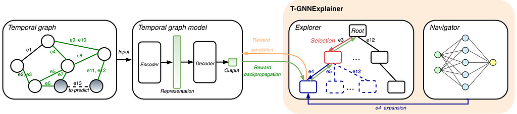
2023 saw the first approaches for explaining temporal GNN methods. Explainers are important for high-stake applications such as fraud detection and disease progression prediction in healthcare. Xia et al. proposed T-GNNExplainer as the first explainer designed for temporal graph models. T-GNNExplainer is model-agnostic and finds important events from a set of candidate events to best explain the model prediction. Xia et al. treat the problem of identifying a subset of explaining events as a combinatorial optimization problem by searching over a subset of the temporal graph within a given size. To tackle this, T-GNNExplainer employs an explorer-navigator framework. The navigator is trained from multiple target events to capture inductive correlations between events while the explorer searches out a specific combination of events based on Monte Carlo Tree Search, including node selection, node expansion, reward simulation and backprop. Which events are pruned is inferred from the navigator. The diagram below shows the framework of T-GNNExplainer.
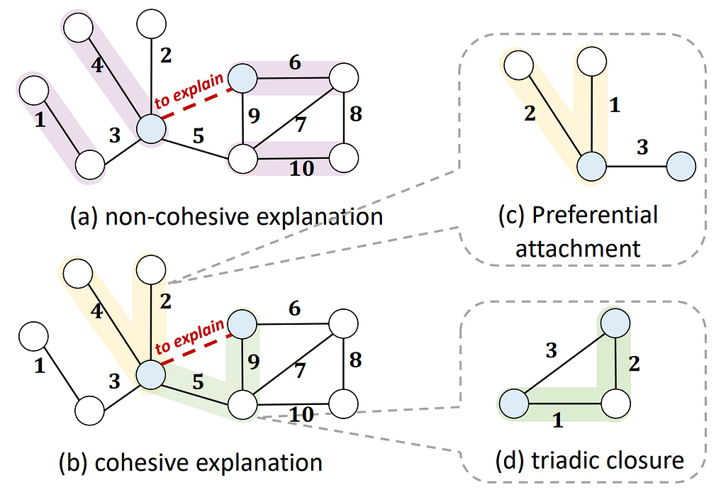
Recently, Chen et al. argued that to form human intelligible explanations for temporal graph events requires the explanation to be events that are temporally proximate and spatially adjacent to that of the prediction, referred to as cohesive explanations. Utilizing temporal motifs, recurring substructures within the temporal graph, is a natural solution to form cohesive explanations for temporal graphs. This is because temporal motifs are crucial factors that guide the generative process of future events. In the following example, the preferential attachment rule (often facilitating influencer effect in e-commerce) and triadic closure rule (explains common-friend rules in social networks) forms cohesive and plausible explanations.
Cohesive explanations are temporally approximate and spatially adjacent. Image source: Chen et al. 2023
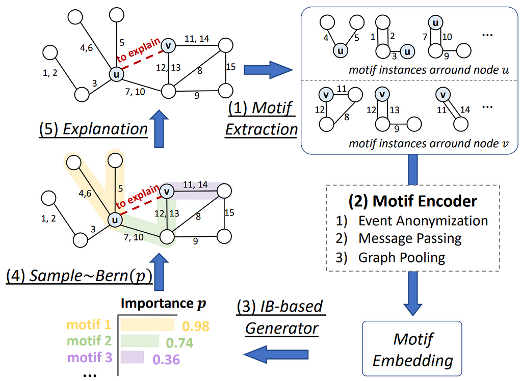
Therefore, Chen et al. proposed TempME, a novel Temporal Motif-based Explainer to identify important temporal motifs to explain temporal GNNs. The framework of TempME is shown in the below figure. First, temporal motifs surrounding the target prediction are extracted. Then these candidate motifs are encoded via the Motif Encoder which leverages event anonymization, message passing and graph pooling to generate an embedding for each motif. Then, based on the Information-bottleneck principle, TempME assigns importance scores to these motifs constrained by both explanation accuracy and information compression. Lastly, explanations are constructed by sampling from the Bernoulli distribution based on the importance score.
Framework of TempME, numbers on the edges denote the temporal order. Image credit: Chen et al. 2023
Adversarial Attacks on Temporal Graphs
“As temporal graphs are adopted to be used for important tasks, like fraud detection, it is important to understand their failure points under adversarial attacks. Understanding and quantifying such blind spots is the first step towards creating robust and reliable temporal GNN models. Such efforts are necessary to ensure industry adoption of these models.” – Srijan Kumar, Assistant Professor at Georgia Institute of Technology
Adversarial attacks can target the privacy of customers or affect critical decisions in financial systems. As temporal graph models are deployed to applications such as recommendation systems and fraud detection, it is important to investigate attacks and design defense mechanisms for TG models. Chen et al. proposed the first adversarial attack for dynamic link prediction called Time-aware Gradient Attack (TGA) for discrete time dynamic graphs. TGA rewires a limited number of links from the original network and the most valuable links to the predicted link are determined by the gradient information generated by the TG model.
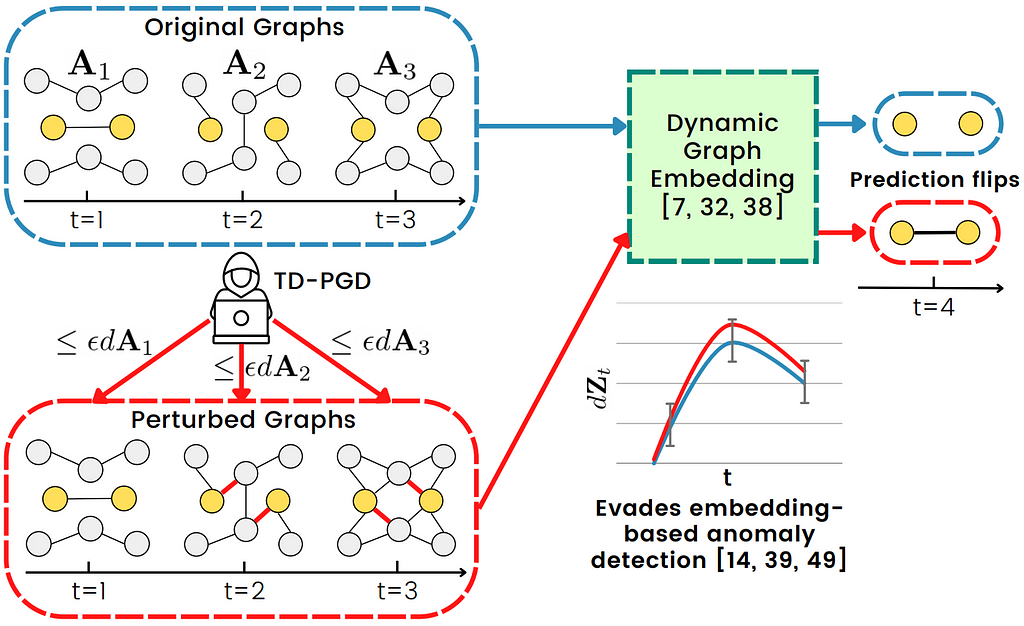
Overview of the Temporal Dynamics-aware Perturbation attack. The attacker can flip the prediction of the model while evading detection. Image source: Sharma et al. 2023
Recently, Sharma et al. argued that effective attacks on temporal graphs must optimize both edge and time perturbations while preserving the original graph evolution. This is because drastic attacks that disturb the graph evolution would be easily detected by anomaly detection methods. Therefore, Sharma et al. formulated evolution-preserving attacks on discrete-time dynamic graphs as the Temporal Dynamics-Aware Perturbation (TDAP) constraint. TDAP asserts that perturbations added at a given timestamp must only be a small fraction of the actual number of changes with respect to the preceding timestamp. TDAP is shown to preserve the rate of change in both the structure and the embedding spaces. An overview of TDAP is shown in the figure below. Sharma et al. then proposes a novel attack method called Temporal Dynamics-aware Projected Gradient Descent (TD-PGD) which is shown to have a closed-form projection operator under the TDAP constraint. An online version of TD-PGD is also proposed where perturbations can be added in real time. Lastly, it is shown empirically that TDAP-constrained perturbations can indeed evade attacks by embedding-based anomaly detection methods.
Libraries and Benchmarks
In 2023 saw a significant push towards standardized libraries and benchmarks for temporal graph learning. TGB provides an open and standardized benchmark for node and link level tasks. DyGLib is a library which includes standard training pipelines, extensible coding interfaces, and comprehensive evaluation strategies for temporal graph learning. Zhang et al. introduced the novel concept of Live Graph Lab, providing live graphs according to blockchain transactions. With a set of tools for downloading, parsing, cleaning, and analyzing blockchain transactions, Live Graph Lab offers researchers the opportunity to extract update to date temporal graph data any time and use it for analysis or testing. Zhou et al. noticed that node memory used in TG models favors small batch sizes and needs to be maintained synchronously across all trainers. Therefore, they proposed DistTGL, an efficient and scalable solution to train memory-based TGNNs on distributed GPU clusters. Enabling multi-GPU training on large datasets is an important direction to deploy TG models on large datasets. We present an updated list of libraries and benchmarks for temporal graph learning:
To join the fast growing TG community, sign up for the weekly temporal graph reading group here. Visit the reading group website and Youtube to see all upcoming and recorded past talks. We also include the invitation link to the TG slack on the website (updated monthly). The second edition of temporal graph learning workshop @ NeurIPS 2023 includes an exciting lineup of 35 posters for cutting edge research in TG. You can also find the talk recordings on the NeurIPS virtual site (will be public in a month). If you want to be a reviewer for the next edition of the workshop, sign up here. To find more about the research from the authors of this post, see our websites: Shenyang(Andy) Huang, Emanuele Rossi, Michael Galkin ,Andrea Cini and Ingo Scholtes. Hope to see you at the reading group or the next edition of the workshop!
Logo of the NeurIPS 2023 Temporal Graph Learning Workshop. Image by authors.
A Case Study Examining the Impact of the Data Act, the GDPR and the AI Act on Connected Cars
One of the newest additions that might make the lives of a lot of smart product manufacturers just a bit more complicated is the EU Data Act,[1] that now comes on top of the GDPR, only to be smushed in a sandwich once the AI act comes into force. Will this sandwich always have all its layers? Well, most certainly not, but this will be the case in a wide variety of situations and for a wide variety of products. Why? To answer this question let’s consider a case study of IntelliCar, a new (fictitious) smart connected car producer, determined to conquer this strong market and some dominant players in it.
DISCLAIMER: This is a work of fiction, however, similarities to companies active or dissolved, or actual technologies implemented in their products are absolutely non-coincidental.
IntelliCar is a European-based company that recently started producing smart cars for the European market. In order to get the desired answer when looking into the magic mirror and asking who has the smartest car of them all, IntelliCar thought long and hard and decided to equip their super smart cars with: facial and emotion recognition automatically adjusting the car temperature and sending warnings when the driver dozes off, optional usage-based car insurance,[2] its very own ChatGPT powered virtual assistant, and a whole bunch of other safety and driving-experience enhancing technologies. However, the three mentioned already suffice to make my point, so I will stop myself here. Now, to be fully honest, any single one of the three listed technologies would be enough to trigger the application of the EU Data Act, the GDPR and the AI Act, but I wanted to mention a couple of interesting provisions of the EU Data Act (the article is going to be more focused on it), so bear with me here.
GDPR
First things first, the situation with the GDPR is pretty straightforward in the described case. We have three technologies in the car all of which will collect (a lot of) personal data.
The car will first collect facial data in order to recognize the user and check whether the driver has given his consent for subsequent processing operations. (Now, we can’t expect IntelliCar to account for this initial act of processing as well, it’s just all too complicated, and the dominant players aren’t paying much attention to it either so surely as a startup, they can afford to look the other way?) If the consent is recorded the car will continue to collect and process the facial expressions in order to adjust the car temperature, send alerts if signs of doziness appear and even ask the driver what’s wrong through its voice assistant feature. Second, if the driver also opted for usage-based insurance the car will collect usage data that can be ascribed to the particular identified and consenting driver. That data will then be transferred to the insurance company for them to process and adjust the insurance premiums. Finally, by saying “Hey IntelliCar (or any name as decided by the user)” the car’s voice assistant activates. Then an almost unlimited number of requests can be made to the car including playing music, asking for directions or even searching things up online, because as you remember our virtual assistant is powered by ChatGPT and hence reasonably capable of performing such requests. All the collected processed data is definitely personal, as the face, the voice and the habits of a particular (already identified) driver, all constitute information based on which someone (most obviously IntelliCar in this case) can identify the driver.
Well, okay not much new there. The GDPR applies to connected cars, of course. There goes the first loaf of bread in our sandwich.
AI Act
The situation with the AI Act is slightly more complicated but, as we’ll see, the gist is that the AI Act still applies. If anything, then to assess whether there are any specific obligations from the Act to comply with.
So, let’s start with the most obvious one. Facial and emotion recognition systems are definitely types of machine-based systems that can generate outputs, such as, in this case, recommendations or decisions that influence the physical environments i.e. car temperature (Article 3). Intellicar is the one that developed and implemented the system and, thus, also its provider. So now it only remains to be determined which (if any) obligations they have to comply with. To answer this question, we can start by confirming that facial and emotion recognition systems are provisionally listed in Annex III as high-risk AI systems. The only way to still potentially get out of all the obligations of the Act would be to conduct a risk assessment and elaborate that their particular system does not actually pose a high risk for the affected persons, as sufficient data protection measures are in place and the recommendations and decisions made by the system are of minor importance. This assessment, even if the result is positive, meaning the system is not that risky after all, will still have to be thorough, documented, and submitted to the authorities though.
The feature recording data for automated insurance adjustments is slightly more complex as here it is not the company that actually has access to or implements the AI system. It simply provides the data (or at least it should). Data providers are (luckily) not a role under the AI Act, so with sufficient contractual and documentation safeguards in place we should be safe. but only given that IntelliCar didn’t in some way significantly re-adjust the system to fit it to their cars, which wouldn’t be all that surprising. In that case, we are back to where we started, IntelliCar is again considered a provider and still has at least some risks to assess.
Finally, our virtual assistant might be the most troublesome of them all, as we have to first determine whether IntelliCar is a deployer or a provider of the technology. For the sake of simplicity let’s say that in this case, IntelliCar uses the ChatGPT Enterprise plug-in and only customizes it using internal data. So hopefully they are just deploying the system and can only be held responsible for choosing a potentially non-compliant system. But they can leave that problem for their future selves. First it is time to conquer the market, whatever the (future) cost.
Data Act
Now finally we come to the last (well definitely not the last, but the last we’ll consider here) secret ingredient in our connected car compliance sandwich. The Data Act. And here our IntelliCar will find itself under attack on all three fronts (pretty straightforwardly) as a manufacturer of a connected product. And just to linger on this Act that received undeservingly little attention in the public, there are multiple booby traps to be on the lookout for here.
The Data Act primarily serves the purpose of empowering users by granting them various access rights not just to the personal data collected during the use of connected products but also to non-personal data, such as data indicating hardware status and malfunctions (Recital 15). Now, although when it comes to connected products, which are most often used by natural persons, it is fairly safe to say that a lot of the collected data will be personal. It is still good to keep in mind that the users have to be able to access ALL collected data (metadata necessary for interpreting the original data included). And this has to be possible easily, securely, free of charge, and, at best, in a comprehensible machine-readable, and directly accessible format. (Piece of cake!) Of course, the Act brings a whole bunch of other obligations, in particular regarding information sharing, depending on the role a particular company (or natural person) has under it. I won’t go into all of them, but I will mention a couple of particularly interesting ones relevant to my imaginary context.
The first one is the way the Act deals with trade secrets. Namely, in situations when the user cannot access the data directly, data has to be provided to the user by the data holder. Now, a lot of this data is going to be very valuable to the company holding it, maybe even as valuable as to put it on the pedestal of a trade secret. These secrets are in fact technical or organizational information that have commercial value, are purposefully kept secret, and to which access is limited. And so, while individual data points might not merit this status, when we think about more complex collections built from collected data points, potentially enriched with third-party data and even inferences, these collections might very well merit trade secret protection. And while the GDPR would never even consider the idea that a user couldn’t access a profile built based on his data, the Data Act does consider this possibility. Primarily because it also governs the sharing of non-personal data. So, in certain cases where the risk of suffering serious economic damage is demonstrated the data holder may withhold the requested data on the basis of it being a trade secret. This exception might leave some wiggle room for the companies to not share all of their valuable data after all.
The second peculiarity concerns our usage-based insurance premium, as the Act also regulates smart contracts. Meaning contracts where “a computer program [is] used for the automated execution of an agreement … using a sequence of electronic records”. One example of such a smart contract could be automated insurance adjustments based on real-time data. And one important obligation in this regard is the smart contract kill switch that has to be implemented as “a mechanism … to terminate the continued execution of transactions and that … includes internal functions which can reset or instruct the contract to stop or interrupt the operation”. This kill switch poses important questions as to the consequences it has for the driver, IntelliCar, as well as the insurance company. Namely, it raises questions such as who is entitled to use the kill switch, when can it be used (contracts are contracts for a reason and their execution is in most cases a good, legally mandated thing), what happens when someone uses it (does the premium fall back to a default mode?), and can clicking the kill switch be reversed (how to account for the unrecorded driving time)? All this will have to be (most likely) contractually regulated between the parties involved and is no trivial matter.
Finally, one last headache we’ll consider is that virtual assistants are also explicitly regulated by the Data Act (Article 31). Virtual assistant, in the context of the act, means “software that can process demands, tasks or questions including those based on audio, written input, gestures or motions, and that, based on those demands, tasks or questions, provides access to other services or controls the functions of connected products”. Now this basically opens up a Pandora’s box not just for our smart car producer but potentially also for the company developing the virtual assistant, possibly dragging them into yet another 70 pages of legislative texts to comply with. (As if they didn’t have enough on their plate already.) And how the trade secret argument (or maybe excuse) would play out in this context can be anybody’s guess.
Final thoughts
As the EU data and technology regulations keep piling up, I have no choice but to imagine how all of them will work together or rather if they can work together at all. Most of all, because complying with all the obligations from all these Acts (whatever did happen to regulations) is no one-man job. Unless that man is a machine (no pun intended) with unlimited brain storage capacity. Already the GDPR is a piece of work compliance-wise, so when we add all these novelties on top, your compliance budget now has to account for a team of lawyers, who are capable of communicating with a team of programmers, who are then able to program all these obligations into a system. The reason I chose smart cars for my example is because all of these technologies exist and are implemented in any single given connected car. And all of the described assessments, obligations, and considerations (just to overstate the complexity point once again) come on top of a whole lot of technical and safety regulations that all cars have to comply with. (Dumb and unconnected ones included.) Now, with all the new features, it appears the connected cars are basically turning into compliance nightmares on four wheels. Nothing else to say than good luck and let the Hunger Games begin!
We use cookies on our website to give you the most relevant experience by remembering your preferences and repeat visits. By clicking “Accept”, you consent to the use of ALL the cookies.
This website uses cookies to improve your experience while you navigate through the website. Out of these, the cookies that are categorized as necessary are stored on your browser as they are essential for the working of basic functionalities of the website. We also use third-party cookies that help us analyze and understand how you use this website. These cookies will be stored in your browser only with your consent. You also have the option to opt-out of these cookies. But opting out of some of these cookies may affect your browsing experience.
Necessary cookies are absolutely essential for the website to function properly. These cookies ensure basic functionalities and security features of the website, anonymously.
Cookie
Duration
Description
cookielawinfo-checkbox-analytics
11 months
This cookie is set by GDPR Cookie Consent plugin. The cookie is used to store the user consent for the cookies in the category "Analytics".
cookielawinfo-checkbox-functional
11 months
The cookie is set by GDPR cookie consent to record the user consent for the cookies in the category "Functional".
cookielawinfo-checkbox-necessary
11 months
This cookie is set by GDPR Cookie Consent plugin. The cookies is used to store the user consent for the cookies in the category "Necessary".
cookielawinfo-checkbox-others
11 months
This cookie is set by GDPR Cookie Consent plugin. The cookie is used to store the user consent for the cookies in the category "Other.
cookielawinfo-checkbox-performance
11 months
This cookie is set by GDPR Cookie Consent plugin. The cookie is used to store the user consent for the cookies in the category "Performance".
viewed_cookie_policy
11 months
The cookie is set by the GDPR Cookie Consent plugin and is used to store whether or not user has consented to the use of cookies. It does not store any personal data.
Functional cookies help to perform certain functionalities like sharing the content of the website on social media platforms, collect feedbacks, and other third-party features.
Performance cookies are used to understand and analyze the key performance indexes of the website which helps in delivering a better user experience for the visitors.
Analytical cookies are used to understand how visitors interact with the website. These cookies help provide information on metrics the number of visitors, bounce rate, traffic source, etc.
Advertisement cookies are used to provide visitors with relevant ads and marketing campaigns. These cookies track visitors across websites and collect information to provide customized ads.