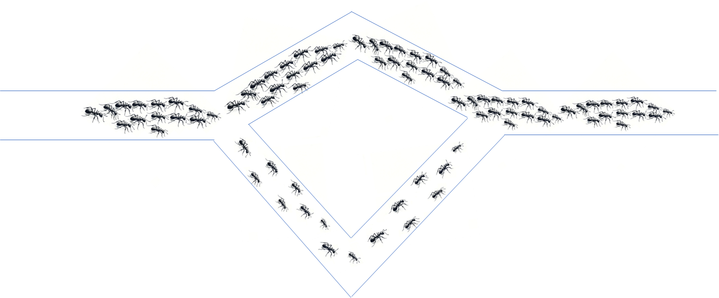
Ant Colony Optimization — Intuition, Code & Visualization
Ant Colony Optimization — Intuition, Code & Visualization


The question is not anymore whether we can solve the problem with AI but to what extent it returns sustainable and reliable results. Good…
Originally appeared here:
To Data or Not to Data.


A technical deep dive into the new deep learning library MLX
Originally appeared here:
Deploying LLMs locally with Apple’s MLX framework
Go Here to Read this Fast! Deploying LLMs locally with Apple’s MLX framework
Metrics to measure the gap between neural text and human text
Originally appeared here:
Evaluating Text Generation in Large Language Models
Go Here to Read this Fast! Evaluating Text Generation in Large Language Models
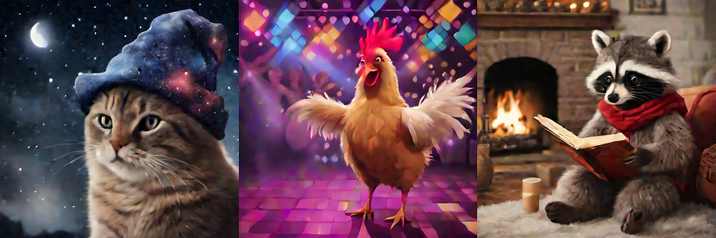
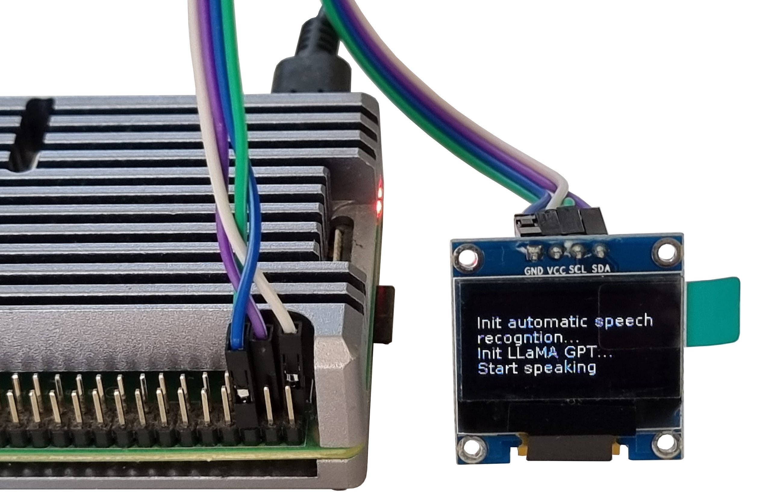
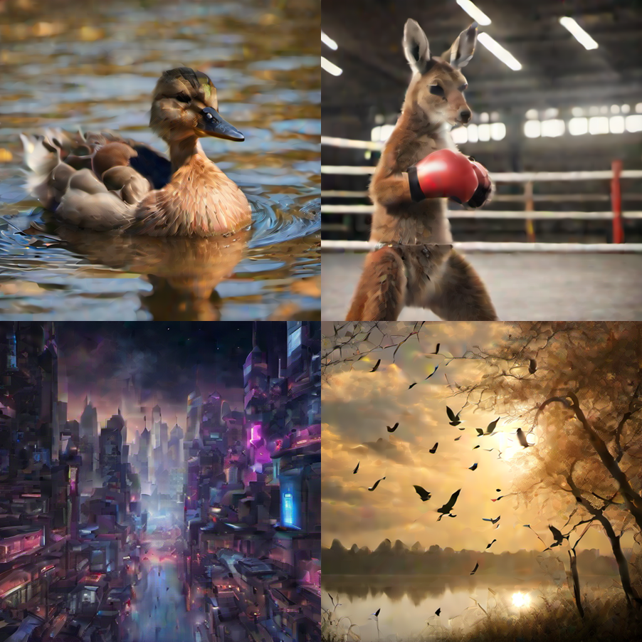
In my last article, I shared how to run large language models and vision language models on the Raspberry Pi. This time around, instead of LLMs and VLMs, we shall run an image generation model — Stable Diffusion XL (SDXL) Turbo — on the Raspberry Pi 5. It’s another impossible sounding feat, but open-source wonders do exist, and running a SDXL Turbo model on a very resource constrained environment is one of them.
OnnxStream is an open-source project created by Vito Plantamura with the original intention of running Stable Diffusion 1.5 (SD1.5) on a Raspberry Pi Zero 2 by minimising memory consumption as much as possible, albeit at the cost of increased inference latency/throughput.
At the time of writing, it has expanded to support not only Stable Diffusion 1.5 but also Stable Diffusion XL 1.0 Base (SDXL) and Stable Diffusion XL Turbo 1.0. I won’t go into detail about how exactly this amazing feat is being achieved since the GitHub repository already explains it very well.
Instead, let’s just jump right into getting it working.
All you need is the following:
The instructions here are from the GitHub repository, but I’m breaking it down and explaining it a bit more.
First, we have to install XNNPack, which is a library from Google that provides “high-efficiency floating-point neural network inference operators”. But we can’t just get the latest version in case of any breaking changes. Instead, we shall get the version that the OnnxStream creator has verified to be working at the time of writing. In a terminal, run:
git clone https://github.com/google/XNNPACK.git
cd XNNPACK
git checkout 579de32260742a24166ecd13213d2e60af862675
mkdir build
cd build
cmake -DXNNPACK_BUILD_TESTS=OFF -DXNNPACK_BUILD_BENCHMARKS=OFF ..
cmake --build . --config Release
XNNPack will take a couple of minutes to build. Go get coffee or something.
Next, we have to build OnnxStream. In a terminal, run:
git clone https://github.com/vitoplantamura/OnnxStream.git
cd OnnxStream
cd src
mkdir build
cd build
cmake -DMAX_SPEED=ON -DXNNPACK_DIR=<DIRECTORY_WHERE_XNNPACK_WAS_CLONED> ..
cmake --build . --config Release
Make sure to replace <DIRECTORY_WHERE_XNNPACK_WAS_CLONED> with the path at which XNNPack was cloned to (not the build folder). In my case, it was at /home/admin/XNNPACK/.
Now, we need to download the model weights for SDXL Turbo. In a terminal, run:
git lfs install
git clone --depth=1 https://huggingface.co/AeroX2/stable-diffusion-xl-turbo-1.0-onnxstream
If you have not installed git-lfs yet, do so first. This will take even longer than the step before since the model weights are quite big. Go get lunch!
You can also run the other two models supported — Stable Diffusion 1.5 and Stable Diffusion XL 1.0 Base by downloading their weights from the links provided in OnnxStream’s GitHub repository. Make sure your SD card has enough space if you are downloading all these models!
Once done, that’s it! We are ready to generate images on a Raspberry Pi!
To generate images, run the code block below:
cd ~/OnnxStream/src/build/
./sd --turbo --models-path /home/admin/stable-diffusion-xl-turbo-1.0-onnxstream --prompt "An astronaut riding a horse on Mars" --steps 1 --output astronaut.png
Replace the prompt with what you want to generate. I’m just using the go-to classic astronaut prompt here. I set steps to just 1 as SDXL Turbo doesn’t need many steps to generate a good-looking image.
There are other arguments you can pass too, such as — neg-prompt for negative prompts (SDXL Turbo does not support negative prompts but you can use it for the other two models), — steps to set the number of generative steps and — seed to set the random seed.
The arguments required will change according to the type of model used, so please take a look at OnnxStream’s GitHub repository for the full list of arguments to pass if you’re using something other than SDXL Turbo.

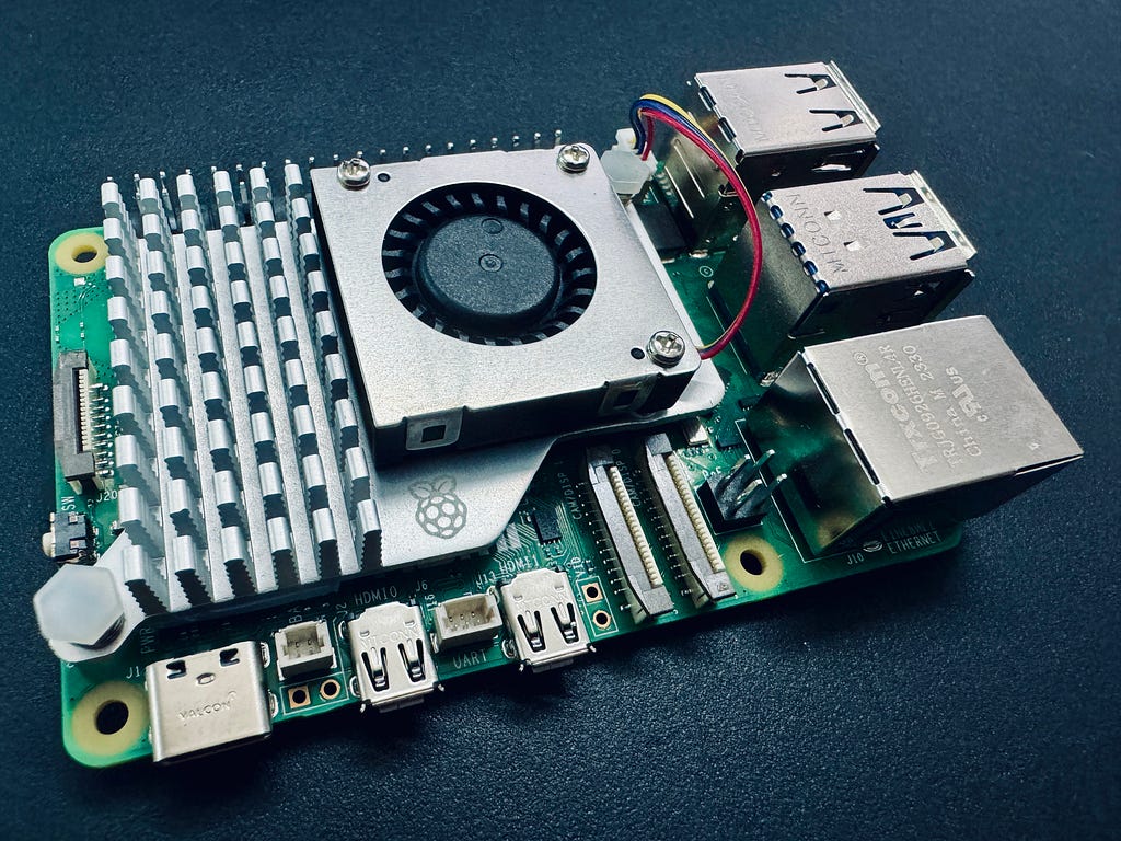
As you can see in the image above, on the Raspberry Pi 5, each diffusion step takes around 1 minute, and in total with pre-processing and decoding, it around 3 minutes to generate a single image.
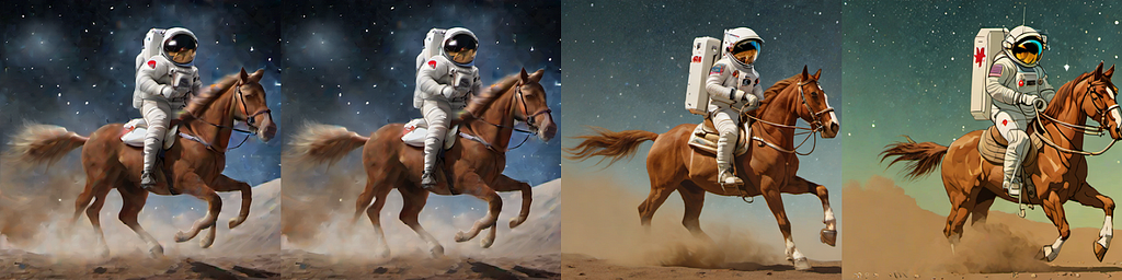
Here’s a comparison and progression of the same prompt with the same seed from step 1 to 10. You can see that even with a single step with refinement, the generated image is already really well-done. This is in contrast to SDXL or SD1.5 which requires quite a few steps to reach that quality.
With it taking around at least a couple of minutes to generate an image, the question of use cases for it comes begging.
The most obvious and fun use case to me is an ever-changing photo frame that will generate a new image every few minutes. There is actually a project along this tangent that uses OnnxStream, by rvdveen on GitHub, where he uses OnnxStream on a Raspberry Pi Zero 2 W to generate images for news articles and shows it on a photo frame using an e-ink display. It takes around 5 hours to generate an image on the Pi Zero 2 W with what should be SD1.5, but hey it’s not like you need a photo frame to be changing what it’s showing in real-time.
Or maybe you just want your own locally hosted image generator which can produce decent quality images while not hogging any major compute devices on your network.
Have fun playing around with SDXL Turbo on the Raspberry Pi!
Disclaimer: I have no affiliation with OnnxStream or StabilityAI. All views and opinions are my own and do not represent any organisation.
Generating Images with Stable Diffusion and OnnxStream on the Raspberry Pi was originally published in Towards Data Science on Medium, where people are continuing the conversation by highlighting and responding to this story.
Originally appeared here:
Generating Images with Stable Diffusion and OnnxStream on the Raspberry Pi

Is being able to build and train machine learning models from popular libraries sufficient for machine learning users? Probably not for too long. With tools like AutoAI on the rise, it is likely that a lot of the very traditional machine learning skills like building model architectures with common libraries like Pytorch will be less important.
What is likely to persist is the demand for skilled users with a deep understanding of the underlying principles of ML, particularly in problems that require novel challenges, customisation, optimisation. To be more innovative and novel, it is important to have a deep understanding of the mathematical foundations of these algorithms. In this article, we’ll look at the mathematical description of one such important model, Recurrent Neural Network (RNN).
Time series data (or any sequential data like language) has a temporal dependencies and is widespread across various sectors ranging from weather prediction to medical applications. RNN is a powerful tool for capturing sequential patterns in such data. In this article, we’ll delve into the mathematical foundations of RNNs and implement these equations from scratch using python.
Understanding RNNs: The Mathematical Description
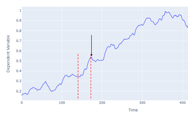
An important element of sequential data is the temporal dependence where the past values determine the current and future values (just like the predetermined world we live in but let’s not get philosophical and stick to RNN models). Time series forecasting utilises this nature of sequential data and focuses on the prediction of the next value given previous n values. Depending on the model, this includes either mapping or regression of the past values.
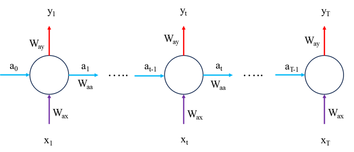
Consider the point indicated with the black arrow, y and the points before y (between the red dashed line) denoting as X = {x1 , x2 , ….xt …..xT} where T is the total number of time steps. The RNN processes the input sequence (X) by placing each input through a hidden state (or sometimes refered to as memory state) and outputs y. These hidden states allow the model to capture and remember patterns from earlier points in the sequence.
Now let’s look at the mathematical operations within the RNN model, first lets consider the forward pass, we’ll worry about the model optimisation later.
Forward Pass
The forward pass is fairly straightforward and is as follows:
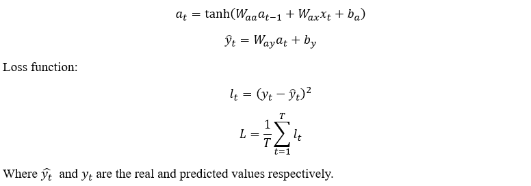
Backpropagation Through Time
In machine learning, the optimisation (variable updates) are done using the gradient descent method:

Therefore, all parameters that need updating during training will require their partial derivatives. Here we’ll derive the partial derivative of the loss function with respect to each variable included in the forward pass equations:

By noting the forward pass equations and network schematic in Figure 2, we can see that at time T, L only depends on a_T via y_T i.e.

However, for t < T, L depends on a_T via y_T and a_(T+1) so let’s use the chain rule for both:
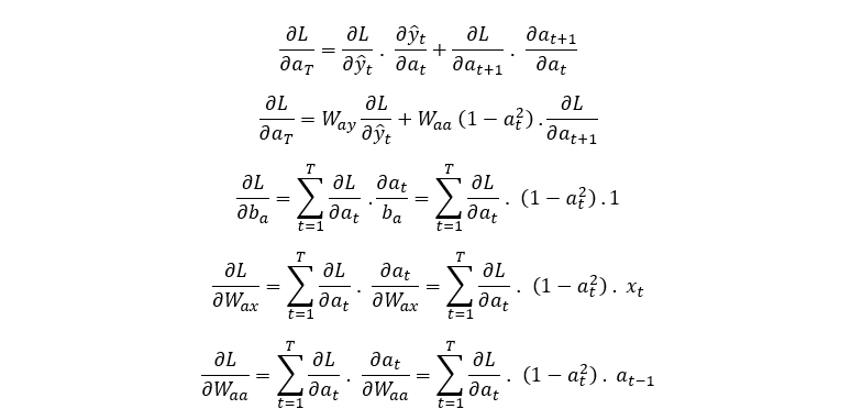
Now we have the equations for the gradient of the loss function with respect all parameters present in the forward pass equation. This algorithm is called Backpropagation Through Time. It is important to clarify that for a time series data, usually only the last value contribute to the Loss function i.e. all other outputs are ignored and their contribution to the loss function set to 0. The mathematical description is the same as that presented. Now Let’s code these equations in python and apply it to an example dataset.
The Coding Implementation
Before we can implement the equations above, we’ll need to import the necessary dataset, preprocess and ready for the model training. All of this work is very standard in any time series analysis.
import numpy as np
import pandas as pd
import matplotlib.pyplot as plt
import plotly.graph_objs as go
from plotly.offline import iplot
import yfinance as yf
import datetime as dt
import math

#### Data Processing
start_date = dt.datetime(2020,4,1)
end_date = dt.datetime(2023,4,1)

#loading from yahoo finance
data = yf.download("GOOGL",start_date, end_date)

pd.set_option('display.max_rows', 4)
pd.set_option('display.max_columns',5)
display(data)


# #Splitting the dataset
training_data_len = math.ceil(len(data) * .8)
train_data = data[:training_data_len].iloc[:,:1]
test_data = data[training_data_len:].iloc[:,:1]

dataset_train = train_data.Open.values
# Reshaping 1D to 2D array
dataset_train = np.reshape(dataset_train, (-1,1))
dataset_train.shape
scaler = MinMaxScaler(feature_range=(0,1))
# scaling dataset
scaled_train = scaler.fit_transform(dataset_train)

dataset_test = test_data.Open.values
dataset_test = np.reshape(dataset_test, (-1,1))
scaled_test = scaler.fit_transform(dataset_test)


X_train = []
y_train = []
for i in range(50, len(scaled_train)):
    X_train.append(scaled_train[i-50:i, 0])
    y_train.append(scaled_train[i, 0])

X_test = []
y_test = []
for i in range(50, len(scaled_test)):
    X_test.append(scaled_test[i-50:i, 0])
    y_test.append(scaled_test[i, 0])

# The data is converted to Numpy array
X_train, y_train = np.array(X_train), np.array(y_train)

#Reshaping
X_train = np.reshape(X_train, (X_train.shape[0], X_train.shape[1],1))
y_train = np.reshape(y_train, (y_train.shape[0],1))
print("X_train :",X_train.shape,"y_train :",y_train.shape)

# The data is converted to numpy array
X_test, y_test = np.array(X_test), np.array(y_test)

#Reshaping
X_test = np.reshape(X_test, (X_test.shape[0], X_test.shape[1],1))
y_test = np.reshape(y_test, (y_test.shape[0],1))
The model
Now we implement the mathematical equations. it is definitely worth reading through the code, noting the dimensions of all variables and respective derivates to give yourself a better understanding of these equations.
class SimpleRNN:
    def __init__(self,input_dim,output_dim, hidden_dim):
        self.input_dim = input_dim
        self.output_dim = output_dim
        self.hidden_dim = hidden_dim
        self.Waa = np.random.randn(hidden_dim, hidden_dim) * 0.01 # we initialise as non-zero to help with training later
        self.Wax = np.random.randn(hidden_dim, input_dim) * 0.01
        self.Way = np.random.randn(output_dim, hidden_dim) * 0.01
        self.ba = np.zeros((hidden_dim, 1))
        self.by = 0 # a single value shared over all outputs #np.zeros((hidden_dim, 1))

    def FeedForward(self, x):
        # let's calculate the hidden states
        a = [np.zeros((self.hidden_dim,1))]
        y = []
        for ii in range(len(x)):

            a_next = np.tanh(np.dot(self.Waa, a[ii])+np.dot(self.Wax,x[ii].reshape(-1,1))+self.ba)
            a.append(a_next)
            y_local = np.dot(self.Way,a_next)+self.by
            y.append(np.dot(self.Way,a_next)+self.by)

        # remove the first a and y values used for initialisation
        #a = a[1:]
        return y, a

    def ComputeLossFunction(self, y_pred, y_actual):
        # for a normal many to many model:
        #loss = np.sum((y_pred - y_actual) ** 2)
        # in our case, we are only using the last value so we expect scalar values here rather than a vector
        loss = (y_pred[-1] - y_actual) ** 2
        return loss

    def ComputeGradients(self, a, x, y_pred, y_actual):
        # Backpropagation through time
        dLdy = []
        dLdby = np.zeros((self.output_dim, 1))
        dLdWay = np.random.randn(self.output_dim, self.hidden_dim)/5.0
        dLdWax = np.random.randn(self.hidden_dim, self.input_dim)/5.0
        dLdWaa = np.zeros((self.hidden_dim, self.hidden_dim))
        dLda = np.zeros_like(a)
        dLdba = np.zeros((self.hidden_dim, 1))

        for t in range(self.hidden_dim-1, 0, -1):
            if t == self.hidden_dim-1:
                dldy = 2*(y_pred[t] - y_actual)
            else:
                dldy = 0
            dLdy.append(dldy)
            #dLdby.append(dldy)
            dLdby += dldy
            #print(dldy.shape)
            dLdWay += np.dot(np.array(dldy).reshape(-1,1), a[t].T)

            # Calculate gradient of loss with respect to a[t]
            if t == self.hidden_dim-1:
                dlda_t= np.dot(self.Way.T, np.array(dldy).reshape(-1,1))

            else:
                dlda_t = np.dot(self.Way.T, np.array(dldy).reshape(-1,1)) + np.dot(self.Waa, dLda[t+1]) * (1 - a[t]**2)
            dLda[t] = dlda_t
            #print(dlda_t.shape)

            rec_term = (1-a[t]*a[t])

            dLdWax += np.dot(dlda_t, x[t].reshape(-1,1))*rec_term
            dLdWaa += np.dot(dlda_t, a[t-1].T)*rec_term
            dLdba += dlda_t*rec_term

        return dLdy[::-1], dLdby[::-1], dLdWay, dLdWax, dLdWaa, dLdba

    def UpdateParameters(self,dLdby, dLdWay, dLdWax, dLdWaa, dLdba,learning_rate):
        self.Waa -= learning_rate * dLdWaa
        self.Wax -= learning_rate * dLdWax
        self.Way -= learning_rate * dLdWay
        self.ba -= learning_rate * dLdba
        self.by -= learning_rate * dLdby

    def predict(self, x, n, a_training):
        # let's calculate the hidden states
        a_future = a_training
        y_predict = []

        # Predict the next n terms
        for ii in range(n):
            a_next = np.tanh(np.dot(self.Waa, a_future[-1]) + np.dot(self.Wax, x[ii]) + self.ba)
            a.append(a_next)
            y_predict.append(np.dot(self.Way, a_next) + self.by)

        return y_predict
Training and Testing the model
input_dim = 1
output_dim = 1
hidden_dim = 50
learning_rate = 1e-3
# Initialize The RNN model
rnn_model = SimpleRNN(input_dim, output_dim, hidden_dim)
# train the model for 200 epochs
for epoch in range(200):
for ii in range(len(X_train)):
y_pred, a = rnn_model.FeedForward(X_train[ii])
loss = rnn_model.ComputeLossFunction(y_pred, y_train[ii])
dLdy, dLdby, dLdWay, dLdWax, dLdWaa, dLdba = rnn_model.ComputeGradients(a, X_train[ii], y_pred, y_train[ii])
rnn_model.UpdateParameters(dLdby, dLdWay, dLdWax, dLdWaa, dLdba, learning_rate)
print(f'Loss: {loss}')
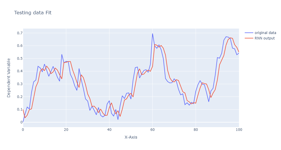
y_test_predicted = []
for jj in range(len(X_test)):
forecasted_values, _ = rnn_model.FeedForward(X_test[jj])
y_test_predicted.append(forecasted_values[-1])
y_test_predicted_flat = np.array([val[0, 0] for val in y_test_predicted])
trace1 = go.Scatter(y = y_test.ravel(), mode ="lines", name = "original data")
trace2 = go.Scatter(y=y_test_predicted_flat, mode = "lines", name = "RNN output")
layout = go.Layout(title='Testing data Fit', xaxis=dict(title='X-Axis'), yaxis=dict(title='Dependent Variable'))
figure = go.Figure(data = [trace1,trace2], layout = layout)
iplot(figure)
That brings us to the end of this demonstration but hopefully only the start of your reading into these powerful models. You might find it helpful to test your understanding by experimenting with a different activation function in the forward pass. Or read further into sequential models like LSTM and transformers which are formidable tools, especially in language-related tasks. Exploring these models can deepen your understanding of more sophisticated mechanisms for handling temporal dependencies. Finally, thank you for taking the time to read this article, I hope you found it useful in your understanding of RNN or their mathematical background.
Unless otherwise noted, all images are by the author
Building Blocks of Time: The Mathematical Foundation and Python Implementation of RNNs was originally published in Towards Data Science on Medium, where people are continuing the conversation by highlighting and responding to this story.
Originally appeared here:
Building Blocks of Time: The Mathematical Foundation and Python Implementation of RNNs


This article explores the relationship between a movie’s dialogue and its genre, leveraging domain-driven data analysis and informed…
Originally appeared here:
Evaluating Cinematic Dialogue — Which syntactic and semantic features are predictive of genre?