Tag: AI

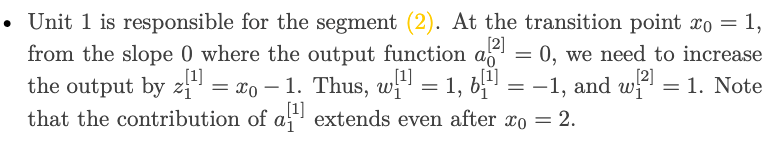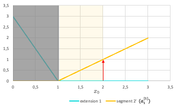
Have you ever wanted to build an assistant that knows when to talk and when to remain silent? Learn how to do it using open-source models.

Intelligent chat assistants have become a central application made possible by the recent generative AI progress, with ChatGPT and Bing Chat/Copilot becoming household names. Typically, this takes the form of a back and forth between a user, who provides prompts or instructions, and an assistant, who in turn provides responses.

A scenario that has received comparatively less attention is one in which an assistant is a semi-active participant in a conversation between two or more users. Examples of such interactions are conversations between groups of friends planning activities together — with the assistant providing recommendations when applicable and staying silent otherwise — or customer support chats, with the assistant providing suggestions to the customer service representative. In these cases, the assistant is not expected to respond at every turn: It would be awkward if it regularly barged in during casual chit-chat between friends.

In this series I’ll go through the steps needed to build a lightweight assistant for this purpose using open-source LLMs. In this context “lightweight” means a model that requires 16GB and 8GB of GPU RAM for training and inference respectively, and that it can efficiently run on a CPU if needed. For this purpose, I will be using Llama-2-7b-hf-chat, Zephyr-7b-beta, and OpenChat-3.5-0106, which all fit this description.

ChatGPT-3.5-Turbo Baseline

To get a feeling for the task we’ll first implement it using ChatGPT. This will give us a reference point from a strong model and will give us an estimate of the task’s difficulty.

Let’s think about some of the unique aspects of our use case:

• We don’t want the assistant to be overzealous: It should only chime in if asked directly or if it has some interesting trivia to add. To this end the assistant needs the possibility to remain silent.
• There are multiple human users in the conversation. To make sense of it, we need to indicate which user is the speaker for each chat message.

For the first aspect we need to define the mechanism for when the assistant chooses to remain silent. To achieve this, we’ll instruct the model to return “(silence)” as its response. Such a prediction can then be filtered during post-processing. An alternative is to ask the model to return an empty prediction, but anecdotally this seems not to be working reliably with some models (they are not used to staying silent!).

For the second aspect, OpenAI’s API conveniently lets us provide the name of the participant for each message in the conversation (curiously this functionality is not exposed in the Playground). This is unfortunately not true for the common open-source models (where we will need a workaround), but for ChatGPT we should be fine.

This leaves one more crucial decision: The prompt. For our use case I’m deliberately picking something short and precise (it can always be adjusted if the tone of the responses ends up being off):

You are an assistant in a group conversation between multiple users.
Your task is to help with relevant information or when directly asked.
Do not be overzealous. If you do not have anything important to say,
respond with "(silence)".

We now have everything we need, let’s give it a try. Using a chat loop as implemented in this notebook, we get the following conversation:

The initial results are encouraging if not perfect: The assistant occasionally chooses to remain silent (adhering to the format from the instructions) or chimes in with helpful information, but it also sometimes responds with unnecessary chit-chat. Changing the prompt to:

You are an assistant in a group conversation between multiple users.
Your task is to help with relevant information or when you are directly
addressed as "assistant". Do not be overzealous, remember that most of
the time the users will be speaking to each other, not to you. If you
do not have anything important to say, respond with "(silence)".

and inserting this reminder system message after every user message:

Remember that the users are most likely to be speaking to each other,
not to you. If you do not have anything important to say, respond with
"(silence)".

does not seem to make a big difference, as seen in this conversation:

It’s likely that the model’s performance can be improved significantly with more work on the prompt, but for now this is sufficient for our purposes: We have a baseline to compare against and we also get an indication that the problem is tractable, if not trivial.

Open-Source Models and Finetuning

We’ve seen that despite some hiccups, ChatGPT-3.5-Turbo is able to act as a semi-active participant in a group conversation. The same is unfortunately not true for common open-source models in the 7B parameter class, which end up responding at every turn. Fortunately, the great thing about open-source LLMs is that we can adapt them to our task via finetuning.

It is worth pointing out that finetuning is not applicable to every situation. For example, if you want to teach a model new facts, finetuning will not be the right tool (a better approach is Retrieval Augmented Generation). However, if you want to alter the tone or format of the responses (as we do here), finetuning is just the thing you need.

Dataset Generation

A critical thing to decide for finetuning is the dataset. We’ll need to provide a set of good examples of multi-user conversations where an assistant largely remains silent, but occasionally chimes in with helpful information. To quickly bootstrap such a set, I enrolled the help of Mixtral-8x7B-Instruct-v0.1, hosted on replicate.com. Specifically, I generated 50 synthetic conversations using this prompt (along with some variations in the topic of discussion and participant names, see this notebook for details):

Generate a conversation representing a chat between two users.
The users are Cynthia and Fred and they are discussing potential
Christmas gifts for friends. An assistant chimes in when it can fill
in trivia, otherwise it remains silent. The conversation should have
between 10 and 12 turns. Return the conversation in a JSON format,
like this:

[
  {
    "role": "user",
    "name": "Alice",
    "content": "Hi Grace! How are you?"
  },
  {
    "role": "user",
    "name": "Grace",
    "content": "I'm good, how about you?"
  },
  {
    "role": "user",
    "name": "Alice",
    "content": "Doing fine as well. I've been reading a book by the author of the Da Vinci code. Sorry, forgot his name"
  },
  {
    "role": "assistant",
    "content": "That’s Dan Brown! He also authored a few other books, for example "Angels & Demons" and "Inferno"."
  }
]

Obviously, the result is not a high quality, curated dataset, so using it for a production model is not recommended. I will discuss some ways to improve the dataset’s quality, as well as approaches for evaluating the resultant model in a subsequent article. However, the dataset is good enough for our purpose right now, that is to validate that a small model can be adapted for the purpose of a multi-user chat assistant.

The dataset generation notebook is available here, and the generated dataset was uploaded to this HuggingFace repository. Below is an example generated dialog:

A Note About Chat Templates

When using a pretrained chat model, it is a good idea to ensure that the format of your input matches the one that the model had been trained with. This has become a bit easier with HuggingFace in September 2023 with the introduction of the apply_chat_template method of the tokenizer. This method takes care of formatting the various user, system and assistant prompts and responses into the required format expected by the model.

Unfortunately, not all models have been updated to have a chat template, so I recommend inspecting the output from apply_chat_template for each model and comparing it to the model’s documentation.

In the context of finetuning (as opposed to just using on off-the-shelf model for inference) we don’t necessarily have to follow a prescribed format. In fact, for non-chat models defining your own chat template is a necessity. However, for chat models sticking with the existing chat template is likely to make the finetuning task easier, resulting in fewer training steps and a smaller possibility of unwanted side effects (think catastrophic forgetting).

For the models we’ve chosen, Zephyr, Llama-7b-chat, and OpenChat-3.5, we are in luck: All of them have their chat templates defined correctly and apply_chat_template works as expected.

Finetuning

We are now ready to kick off the finetuning. As mentioned before, the goal is to fit the training into 16GB of GPU memory, allowing it to run on a single T4 GPU (no need to hunt for the ultra-rare Pokémon… err, I mean A100s). To achieve this, we’ll use 4-bit quantization and LoRA. If you’re unfamiliar with these terms, I highly recommend this article as an introduction. This section will go through the main steps needed for finetuning, the complete training notebook can be accessed here.

Before starting training, we need to slightly massage the synthetic dataset created earlier:

• We need to add information about who the speaker is in each user turn. Remember the helpful name field in OpenAI’s API that allowed us to differentiate between various human speakers? It’s sadly not present in Zephyr’s, Llama’s and OpenChat’s chat templates. As a workaround we will just prepend “{name}: ” at the start of each line.
• We also need to add assistant lines saying “(silence)” every time the assistant chooses not to respond in a turn. In addition, we will also prepend “(response)” before each assistant line. This is not strictly necessary for the basic chat case but will allow us to cajole the model into answering even if it preferred to remain silent (this will come handy during evaluation but can also be a product feature).
• Finally, we also need to apply the chat template.

The dataset preprocessing is implemented as follows:

from transformers import AutoTokenizer

tokenizer = AutoTokenizer.from_pretrained(HF_BASE_MODEL_NAME, use_fast=False)

from datasets import Dataset
from huggingface_hub import hf_hub_download
import json

def build_dataset():
    local_filename = hf_hub_download(
        repo_id=HF_DATASET_NAME,
        filename=HF_DATA_FILE_NAME
    )
    with open(local_filename) as f:
        conversations = f.readlines()
        result = []
        for conversation in conversations:
            lines = json.loads(conversation)
            transformed_lines = []

            idx = 0
            while idx < len(lines):
                assert lines[idx]['role'] == 'user'
                transformed_lines.append({
                    'role': 'user',
                    'content': f"{lines[idx]['name']}: {lines[idx]['content']}",
                })

                idx += 1

                if idx == len(lines) or lines[idx]['role'] != 'assistant':
                    # Insert artificial (silence) response
                    transformed_lines.append({
                        'role': 'assistant',
                        'content': '(silence)',
                    })
                else:
                    transformed_lines.append({
                        'role': 'assistant',
                        'content': f"(response) {lines[idx]['content']}",
                    })
                    idx += 1

            result_row = {
                'text': tokenizer.apply_chat_template(tokenize=False, conversation=transformed_lines)
            }
            result.append(result_row)

    return result

dataset = Dataset.from_list(build_dataset())

Note that no system prompt is included. The reason is that we’re finetuning a model for this one specific task, so providing the instructions to the model is redundant: It learns what it is supposed to do from its training. This has the nice side effect of both shorter training and slightly quicker inference.

Having finished preparing the dataset, we now load the quantized model:

import torch
from transformers import AutoModelForCausalLM

torch_compute_type = torch.bfloat16 if USE_BFLOAT16 else torch.float16

model = AutoModelForCausalLM.from_pretrained(
    active_config['base_model_name'],
    torch_dtype=torch_compute_type,
    bnb_4bit_quant_type='nf4',
    bnb_4bit_compute_dtype=torch_compute_type,
    load_in_4bit=True,
    device_map={'':0},
    trust_remote_code=True,
    use_cache=True
)

We then define the adapter model (i.e. the low rank “diff” from the base model):

from peft import LoraConfig, get_peft_model

peft_config = LoraConfig(
        lora_alpha=16,
        lora_dropout=0.1,
        r=64,
        bias="none",
        task_type="CAUSAL_LM",
)

# Note: This is needed for Zephyr, otherwise we get this:
#       RuntimeError: element 0 of tensors does not require grad and does not have a grad_fn
model.enable_input_require_grads()
peft_model = get_peft_model(model, peft_config)

and instantiate the trainer and the training arguments:

from transformers import TrainingArguments

output_dir = "peft_model"

# These arguments (LR, gradient norm, etc.) seem to be fairly frequently
# used for QLoRA. Default arguments work too, but require about 50% more
# epochs. Also tried optim='lion_32bit' out of curiosity, the result was
# pretty much the same as the default (AdamW), but each epoch was 30-40%
# slower.
training_args = TrainingArguments(
    output_dir=output_dir,
    num_train_epochs=TRAIN_EPOCHS,
    per_device_train_batch_size=4,
    gradient_accumulation_steps=2,
    gradient_checkpointing=True,
    logging_steps=1,
    bf16=USE_BFLOAT16,
    #optim='lion_32bit',
    learning_rate=2e-4,
    max_grad_norm=0.3,
    warmup_ratio=0.03,
    lr_scheduler_type="constant",
)

The settings used above are fairly standard (and I encourage you to tweak them as needed). The ones that really matter are the number of epochs, the learning rate, and the batch size. The above is a particular configuration that worked for me and might be a good starting point but is obviously not a substitute for a real hyperparameter search.

We are now ready to instantiate the trainer and kick off the training:

from trl import SFTTrainer

max_seq_length = 1024

trainer = SFTTrainer(
    model=peft_model,
    train_dataset=dataset,
    peft_config=peft_config,
    max_seq_length=max_seq_length,
    tokenizer=tokenizer,
    args=training_args,
    dataset_text_field='text',
)

trainer.train()

That was quick, just 8 minutes on a T4! Let’s test how it does by creating a conversational pipeline and a loop, using the same notebook as for the OpenAI API case. Here is an example conversation using a model finetuned from OpenChat-3.5–0106:

This is pretty encouraging: The model follows our format requirements and seems to make reasonable decisions on when to chime in and when to remain silent.

So — are we done? One thing to note about the training is that the model is taught to predict all of the tokens in each sample, including the user messages and any special tokens. The following section will show how this can be suppressed.

Training on Completions Only

First things first: Why do we even care about not teaching the model to predict the user messages? One argument can be made on the grounds of privacy: If real conversations are used as training data, a model could possibly be persuaded by an end user to leak some of the user messages (for what it’s worth, assistant responses can contain sensitive information as well). A second argument is that trying to predict user messages is unnecessary, and as a result wasteful. This can mean that you will need to train for a longer time to get good results, and hence risk unwanted side effects (again, this is chiefly catastrophic forgetting).

Depending on your use case both of these arguments might be moot, and the model might do well with the training procedure described above. If, however, it’s not, or if you are just curious, I encourage you to keep reading.

HuggingFace’s trl library provides us with a tool to solve this particular problem, implemented as DataCollatorForCompletionsOnlyLM. This collator changes the labels for the tokens representing user messages to an “ignore” label, meaning the models are not trained to predict them. The user messages are of course still used as context for predicting assistant messages.

DataCollatorForCompletionsOnlyLM requires us to pass two strings that it can use to find the start of the user messages (the instruction_template parameter) and the assistant messages (response_template). We can find them by inspecting the output of apply_chat_template: In the case of Zephyr, they are “<|user|>” and “<|assistant|>”, for Llama they are “[INST]” and “[/INST]”. Let’s try it out:

trainer.data_collator = DataCollatorForCompletionOnlyLM(
    response_template="<|assistant|>",
    instruction_template="<|user|>",
    tokenizer=tokenizer
)

trainer.train()

### Output:
# UserWarning: Could not find response key `<|assistant|>` in the following instance: [...] This instance will be ignored in loss calculation. Note, if this happens often, consider increasing the `max_seq_length`.

Uh oh, this looks bad. Essentially the trainer cannot find our template fragments and as a result ignores all our samples. The reason for this is explained in this article: Depending on the preceding context, a string like “<|user|>” can have different tokenized representations. Fortunately, DataCollatorForCompletionsOnlyLM allows us to pass the tokenized versions of these delimiter strings instead of the literal ones. In order to find these tokenized versions, we can inspect the tokenized output of a chat template:

conversation = [
  { 'role': 'user', 'content': "hi!" },
  { 'role': 'assistant', 'content': "Hello!" }
]

for token in tokenizer.apply_chat_template(conversation):
    print(f"Token Id: {token}, Value: '{tokenizer.decode([token])}'")

### Output
# Token Id: 523, Value: '<'
# Token Id: 28766, Value: '|'
# Token Id: 1838, Value: 'user'
# Token Id: 28766, Value: '|'
# Token Id: 28767, Value: '>'
# Token Id: 13, Value: '
# '
# Token Id: 5365, Value: 'hi'
# Token Id: 28808, Value: '!'
# Token Id: 2, Value: '</s>'
# Token Id: 28705, Value: ''
# Token Id: 13, Value: '
# '
# Token Id: 28789, Value: '<'
# Token Id: 28766, Value: '|'
# Token Id: 489, Value: 'ass'
# Token Id: 11143, Value: 'istant'
# Token Id: 28766, Value: '|'
# Token Id: 28767, Value: '>'
# Token Id: 13, Value: '
# '
# Token Id: 16230, Value: 'Hello'
# Token Id: 28808, Value: '!'
# Token Id: 2, Value: '</s>'
# Token Id: 28705, Value: ''
# Token Id: 13, Value: '
# '

From the output we can infer that “<|assistant|>” is tokenized as [28789, 28766, 489, 11143, 28766, 28767], and “<|user|>” is tokenized as [28789, 28766, 1838, 28766, 28767]. I have included the tokenized sequences for a few common models in the table below.

With this in hand, we can now retry training using the updated data collator:

response_template = [28789, 28766, 489, 11143, 28766, 28767]
instruction_template = [28789, 28766, 1838, 28766, 28767]

trainer.data_collator = DataCollatorForCompletionOnlyLM(
    response_template=response_template,
    instruction_template=instruction_template,
    tokenizer=tokenizer
)

trainer.train()

This gets rid of the warning and the training loss starts decreasing. We can now wait for the model training to finish and upload the model to HuggingFace Hub.

peft_model.push_to_hub(active_config['finetuned_model_name'])
tokenizer.push_to_hub(active_config['finetuned_model_name'])

Smoke Testing

Let’s now see how the model is doing in practice by running this notebook (which can be executed locally using a consumer grade 8GB GPU). Here is an example conversation, again for a model finetuned from OpenChat-3.5–0106:

So — are we done now? This depends on the goal: We do have a model that I like to call “syntactically competent”, meaning that it follows our defined format and is able to decide when to talk and when to remain silent. If the goal is a toy assistant, this might be sufficient. However, for any serious production use, there is still a fair amount of work to do, which I’ll discuss in subsequent articles.

Follow-ups

Let’s list some of the things that are worth consideration as follow-up steps:

• High quality training set: So far, we have only used a synthetic training set generated by Mixtral. This set does not have too much variation and may contain falsehoods. It was useful for bootstrapping but is insufficient for production use.
• Evaluation: So far, we’ve only done a few smoke tests, but we don’t have a good grasp of how the model is performing: Is it responding truthfully, is it doing a good job in determining when to chime in? We also don’t know how much the finetuned model diverged from the base one. In a follow-up article I’ll show how to shed some light on these questions.
• Context: We cannot expect a model with just 7B parameters to be knowledgeable on every topic. In fact, for practical purposes, we may want to constrain the model to particular topics relevant to our product. To this end, we may want to provide contextual information to our model that is relevant to the users’ questions and condition the model to only answer based on this information. This approach is known as Retrieval Augmented Generation (RAG), and I’ll show how it can be applied in our multi-user setting.

Resources and Artifacts

The notebooks used for training and evaluation are available on Colab: Dataset generation, training and inference.

The synthetic dataset is available here.

Finally, the models are available on HuggingFace, finetuned from Zephyr, Llama-2 and OpenChat-3.5. If you are interested in the models trained on whole conversations (as opposed to completions only), they are available as well, finetuned from Zephyr, Llama-2 and OpenChat-3.5.

Troubleshooting

Below I’m listing some pitfalls that I’ve encountered frequently during finetuning, these might come handy when finetuning other models.

Pad Token

I’ve seen the pad token set to the EOS token in multiple tutorials (and also by default in the Zephyr model). This doesn’t play well with HuggingFace’s data collators though: this line in DataCollatorForLanguageModeling means that models are not trained to predict pad tokens. If the pad and EOS tokens are the same, you might end up with a model that continues generating tokens without stopping. My recommendation is to set the pad token to the UNK token if available (and distinct from EOS). Alternatively, you can use the tokenizer’s add_token method to add it to the vocabulary.
In short: Make sure the pad token is not the same as the EOS token. Recent versions of HuggingFace started adding this warning, which adds visibility to the issue:

UserWarning: The pad_token_id and eos_token_id values of this tokenizer are identical. If you are planning for multi-turn training, it can result in the model continuously generating questions and answers without eos token. To avoid this, set the pad_token_id to a different value.

Loss Falling to 0.0 During Training

When using half precision floats (that is torch.float16), I’ve seen situations where the loss goes to 0.0 after a few steps and remains there. Specifically, this happens with our training notebook with the Llama-2 model. There are reports online of similar issues (for example here), curiously they were resolved at that time by setting the tokenizer’s padding_side to “right”. In our case the padding is already on the right-hand side, so that fix does not apply.

The workaround is to use a different type for training: Either torch.bfloat16 (which is unavailable on older instances like T4 and V100) or torch.float32 (which results in a performance hit at training time, but otherwise works fine).

“RuntimeError: element 0 of tensors does not require grad…”

Depending on the model, you might come across this error:

RuntimeError: element 0 of tensors does not require grad and does not have a grad_fn

The simple fix is to add this line after instantiating the model:

model.enable_input_require_grads()

---

AI for Groups: Build a Multi-User Chat Assistant Using 7B-Class Models was originally published in Towards Data Science on Medium, where people are continuing the conversation by highlighting and responding to this story.

Amazon Textract is a machine learning (ML) service that enables automatic extraction of text, handwriting, and data from scanned documents, surpassing traditional optical character recognition (OCR). It can identify, understand, and extract data from tables and forms with remarkable accuracy. Presently, several companies rely on manual extraction methods or basic OCR software, which is tedious […]

Data augmentation for data-deficient deep neural networks.

By: Ian Stebbins, Benjamin Goldfried, Ben Maizes

Intro

Often for many domain-specific problems, a lack of data can hinder the effectiveness and even disallow the use of deep neural networks. Recent architectures of Generative Adversarial Networks (GANs), however, allow us to synthetically augment data, by creating new samples that capture intricate details, textures, and variations in the data distribution. This synthetic data can act as additional training input for deep neural networks, thus making domain tasks with limited data more feasible.

In this project, we applied NVIDIA StyleGAN-2 with Adaptive Discriminator Augmentation (ADA) to a small Chest CT-Scan Dataset (Licensed under Database: Open Database, Contents: © Original Authors)[1]. Additionally, we built a CNN classifier to distinguish normal scans from those with tumors. By injecting varying proportions of synthetically generated data into the training of different models, we were able to evaluate the performance differences between models with all real data and those with a real-synthetic mix.

StyleGAN-2 ADA

StyleGAN-2 with ADA was first introduced by NVIDIA in the NeurIPS 2020 paper: “Training Generative Adversarial Networks with Limited Data” [2]. In the past, training GANs on small datasets typically led to the network discriminator overfitting. Thus rather than learning to distinguish between real and generated data, the discriminator tended to memorize the patterns of noise and outliers of the training set, rather than learn the general trends of the data distribution. To combat this, ADA dynamically adjusts the strength of data augmentation based on the degree of overfitting observed during training. This helps the model to generalize better and leads to better GAN performance on smaller datasets.

Augmenting The Dataset

To use the StyleGAN-2 ADA model, we used the official NVIDIA model implementation from GitHub, which can be found here. Note that this is the StyleGAN-3 repo but StyleGAN-2 can still be run.

!git clone https://github.com/NVlabs/stylegan3

Depending on your setup you may have to install dependencies and do some other preprocessing. For example, we chose to resize and shrink our dataset images to 224×224 since we only had access to a single GPU, and using larger image sizes is much more computationally expensive. We chose to use 224×224 because ResNet, the pre-trained model we chose for the CNN, is optimized to work with this size of image.

!pip install pillow
from PIL import Image
import os

'''Loops through the files in an input folder (input_folder), resizes them to a
specified new size (new_size), an adds them to an output folder (output_folder).'''
def resize_images_in_folder(input_folder, output_folder, new_size):
    # Loop through all files in the input folder
    for filename in os.listdir(input_folder):
        input_path = os.path.join(input_folder, filename)

        # Check if the file is an image
        if os.path.isfile(input_path) and filename.lower().endswith(('.png', '.jpg', '.jpeg', '.gif')):
            # Open the image file
            image = Image.open(input_path)

            #Convert to RGB
            image = image.convert('RGB')

            # Resize the image
            resized_image = image.resize(new_size)

            # Generate the output file path
            output_path = os.path.join(output_folder, filename)

            # Save the resized image to the output folder
            resized_image.save(output_path)

            print(f"Resized {filename} and saved to {output_path}")

To begin the training process, navigate to the directory where you cloned the repo and then run the following.

import os

!python dataset_tool.py --source= "Raw Data Directory" --dest="Output Directory" --resolution='256x256'

# Training
EXPERIMENTS = "Output directory where the Network Pickle File will be saved""
DATA = "Your Training DataSet Directory"
SNAP = 10
KIMG = 80

# Build the command and run it
cmd = f"/usr/bin/python3 /content/stylegan3/train.py --snap {SNAP} --outdir {EXPERIMENTS} --data {DATA}  --kimg {KIMG} --cfg stylegan2 --gpus 1 --batch 8 --gamma 50"
!{cmd}

SNAP refers to the number of Ticks (training steps where information is displayed) after which you would like to take a snapshot of your network and save it to a pickle file.

KIMG refers to the number of thousands of images you want to feed into your GAN.

GAMMA determines how strongly the regularization affects the discriminator.

Once your model has finished training (this can take multiple hours depending on your compute resources) you can now use your trained network to generate images.

pickle_file = "Network_Snapshot.pkl"
model_path = f'Path to Pickle File/{pickle_file}'
SAMPLES = Number of samples you want to generate
!python /content/stylegan3/gen_images.py --outdir=Output Directory --trunc=1 --seeds {SAMPLES} 
    --network=$model_path

Transfer Learning & Convolutional Neural Network

To benchmark the effectiveness of our synthetically generated data, we first trained a CNN model on our original data. Once we had a benchmark accuracy on the test set, we re-trained the model with increasing amounts of synthetic data in the training mix.

To feed our data into the model we used Keras data generators which flow the samples directly from a specified directory into the model. The original dataset has 4 classes for different types of cancer, however, for simplicity, we turned this into a binary classification problem. The two classes we decided to work with from the original Kaggle dataset were the normal and squamous classes.

# Define directories for training, validation, and test datasets
train_dir = 'Your training data directory'
test_dir = 'Your testing data directory'
val_dir = 'Your validation data directory'

# Utilize data genarators to flow directly from directories
train_generator = train_datagen.flow_from_directory(
    train_dir,
    target_size=(224, 224),
    batch_size=20,
    class_mode='binary',  #Use 'categorical' for multi-class classification
    shuffle=True,
    seed=42 )

val_generator = val_datagen.flow_from_directory(
    val_dir,
    target_size=(224, 224),
    batch_size=20,
    class_mode='binary',
    shuffle=True )

test_generator = test_datagen.flow_from_directory(
    test_dir,
    target_size=(224, 224),
    batch_size=20,
    class_mode='binary',
    shuffle=True )

To build our model, we began by using the ResNet50 base architecture and model weights. We chose to use ResNet50 due to its moderate-size architecture, good documentation, and ease of use through Keras. After importing ResNet50 with the Imagenet model weights, we then froze the ResNet50 layers and added trainable dense layers on top to help the network learn our specific classification task.

We also chose to incorporate batch normalization, which can lead to faster convergence and more stable training by normalizing layer inputs and reducing internal covariate shift [3]. Additionally, it can provide a regularization effect that can help prevent overfitting in our added trainable dense layers.

Originally, our model was not performing well. We solved this issue by switching our activation function from ReLU to leaky ReLU. This suggested that our network may have been facing the dying ReLU or dead neuron problem. In short, since the gradient of ReLU will always be zero for negative numbers, this can lead to neurons “dying” and not contributing to the network [4][5]. Since leaky ReLU is nonzero for negative values, using it as an activation function can help combat this issue.

Results

To test our synthetic data, we trained the above CNN on 5 separate instances with 0%, 25%, 50%, 75%, and 100% additional synthetic samples. For example, 0% synthetic samples meant that the data was all original, while 100% meant the training set contained equal amounts of original and synthetic data. For each network, we then evaluated the performance using an accuracy metric on a real set of unseen test data. The plot below visualizes how different proportions of synthetic data affect the testing accuracy.

Training the model was unstable, thus we ruled out iterations where the accuracy was 1.0 or extremely low. This helped us avoid training iterations that were under or over fit.

We can see that from 0 to 25% we see a sharp increase in the testing accuracy, suggesting that even augmenting the dataset by a small amount can have a large impact on problems where the data is initially minimal.

Since we only trained our GAN on 80 KIMG (due to compute limitations) the quality of our synthetic data could have potentially been better, given more GAN training iterations. Notably, an increase in synthetic data quality could also influence the graph above. We hypothesize that an increase in synthetic quality will also lead to an increase in the optimal proportion of synthetic data used in training. Further, if the synthetic images were better able to fit the real distribution of our training data, we could incorporate more of them in model training without overfitting.

Conclusion

In this project, using GANs for the augmentation of limited data has shown to be an effective technique for expanding training sets and more importantly, improving classification accuracy. While we opted for a small and basic problem, this could easily be upscaled in a few ways. Future work may include using more computational resources to get better synthetic samples, introducing more classes into the classification task (making it a multi-class problem), and experimenting with newer GAN architectures. Regardless, using GANs to augment small datasets can now bring many previously data-limited problems into the scope of deep neural networks.

Kaggle Dataset

We compiled our augmented and resized images into the following Kaggle dataset. This contains 501 normal and 501 squamous 224×224 synthetic images which can be used for further experimentation.

Our GitHub Repo

Citations

[1] Hany, Mohamed, Chest CT-Scan images Dataset, Kaggle (2020).

[2] Karras, Tero, et al, Training Generative Adversarial Networks with Limited Data (2020), Advances in neural information processing systems 2020.

[3] Ioffe, Sergey, and Christian Szegedy, Batch normalization: Accelerating deep network training by reducing internal covariate shift, (2015), International conference on machine learning. pmlr, 2015.

[4] He, Kaiming, et al, Delving deep into rectifiers: Surpassing human-level performance on imagenet classification, (2015), Proceedings of the IEEE international conference on computer vision. 2015.

[5]Bai, Yuhan, RELU-function and derived function review, (2022), SHS Web of Conferences. Vol. 144. EDP Sciences, 2022.

---

Enhancing Cancer Detection with StyleGAN-2 ADA was originally published in Towards Data Science on Medium, where people are continuing the conversation by highlighting and responding to this story.

Learn how a neural network with one hidden layer using ReLU activation can represent any continuous nonlinear functions.

Activation functions play an integral role in Neural Networks (NNs) since they introduce non-linearity and allow the network to learn more complex features and functions than just a linear regression. One of the most commonly used activation functions is Rectified Linear Unit (ReLU), which has been theoretically shown to enable NNs to approximate a wide range of continuous functions, making them powerful function approximators.

In this post, we study in particular the approximation of Continuous NonLinear (CNL) functions, the main purpose of using a NN over a simple linear regression model. More precisely, we investigate 2 sub-categories of CNL functions: Continuous PieceWise Linear (CPWL), and Continuous Curve (CC) functions. We will show how these two function types can be represented using a NN that consists of one hidden layer, given enough neurons with ReLU activation.

For illustrative purposes, we consider only single feature inputs yet the idea applies to multiple feature inputs as well.

ReLU activation

ReLU is a piecewise linear function that consists of two linear pieces: one that cuts off negative values where the output is zero, and one that provides a continuous linear mapping for non negative values.

Continuous piecewise linear function approximation

CPWL functions are continuous functions with multiple linear portions. The slope is consistent on each portion, than changes abruptly at transition points by adding new linear functions.

In a NN with one hidden layer using ReLU activation and a linear output layer, the activations are aggregated to form the CPWL target function. Each unit of the hidden layer is responsible for a linear piece. At each unit, a new ReLU function that corresponds to the changing of slope is added to produce the new slope (cf. Fig.2). Since this activation function is always positive, the weights of the output layer corresponding to units that increase the slope will be positive, and conversely, the weights corresponding to units that decreases the slope will be negative (cf. Fig.3). The new function is added at the transition point but does not contribute to the resulting function prior to (and sometimes after) that point due to the disabling range of the ReLU activation function.

Example

To make it more concrete, we consider an example of a CPWL function that consists of 4 linear segments defined as below.

To represent this target function, we will use a NN with 1 hidden layer of 4 units and a linear layer that outputs the weighted sum of the previous layer’s activation outputs. Let’s determine the network’s parameters so that each unit in the hidden layer represents a segment of the target. For the sake of this example, the bias of the output layer (b2_0) is set to 0.

Continuous curve function approximation

The next type of continuous nonlinear function that we will study is CC function. There is not a proper definition for this sub-category, but an informal way to define CC functions is continuous nonlinear functions that are not piecewise linear. Several examples of CC functions are: quadratic function, exponential function, sinus function, etc.

A CC function can be approximated by a series of infinitesimal linear pieces, which is called a piecewise linear approximation of the function. The greater the number of linear pieces and the smaller the size of each segment, the better the approximation is to the target function. Thus, the same network architecture as previously with a large enough number of hidden units can yield good approximation for a curve function.

However, in reality, the network is trained to fit a given dataset where the input-output mapping function is unknown. An architecture with too many neurons is prone to overfitting, high variance, and requires more time to train. Therefore, an appropriate number of hidden units must not be too small to properly fit the data, nor too large to lead to overfitting. Moreover, with a limited number of neurons, a good approximation with low loss has more transition points in restricted domain, rather than equidistant transition points in an uniform sampling way (as shown in Fig.10).

Wrap up

In this post, we have studied how ReLU activation function allows multiple units to contribute to the resulting function without interfering, thus enables continuous nonlinear function approximation. In addition, we have discussed about the choice of network architecture and number of hidden units in order to obtain a good approximation result.

I hope that this post is useful for your Machine Learning learning process!

Further questions to think about:

1. How does the approximation ability change if the number of hidden layers with ReLU activation increase?
2. How ReLU activations are used for a classification problem?

*Unless otherwise noted, all images are by the author

---

How ReLU Enables Neural Networks to Approximate Continuous Nonlinear Functions? was originally published in Towards Data Science on Medium, where people are continuing the conversation by highlighting and responding to this story.