Posted by Rajat Sen and Yichen Zhou, Google Research
Time-series forecasting is ubiquitous in various domains, such as retail, finance, manufacturing, healthcare and natural sciences. In retail use cases, for example, it has been observed that improving demand forecasting accuracy can meaningfully reduce inventory costs and increase revenue. Deep learning (DL) models have emerged as a popular approach for forecasting rich, multivariate, time-series data because they have proven to perform well in a variety of settings (e.g., DL models dominated the M5 competition leaderboard).
At the same time, there has been rapid progress in large foundation language models used for natural language processing (NLP) tasks, such as translation, retrieval-augmented generation, and code completion. These models are trained on massive amounts of textual data derived from a variety of sources like common crawl and open-source code that allows them to identify patterns in languages. This makes them very powerful zero-shot tools; for instance, when paired with retrieval, they can answer questions about and summarize current events.
Despite DL-based forecasters largely outperforming traditional methods and progress being made in reducing training and inference costs, they face challenges: most DL architectures require long and involved training and validation cycles before a customer can test the model on a new time-series. A foundation model for time-series forecasting, in contrast, can provide decent out-of-the-box forecasts on unseen time-series data with no additional training, enabling users to focus on refining forecasts for the actual downstream task like retail demand planning.
To that end, in “A decoder-only foundation model for time-series forecasting”, we introduce TimesFM, a single forecasting model pre-trained on a large time-series corpus of 100 billion real world time-points. Compared to the latest large language models (LLMs), TimesFM is much smaller (200M parameters), yet we show that even at such scales, its zero-shot performance on a variety of unseen datasets of different domains and temporal granularities come close to the state-of-the-art supervised approaches trained explicitly on these datasets. Later this year we plan to make this model available for external customers in Google Cloud Vertex AI.
A decoder-only foundation model for time-series forecasting
LLMs are usually trained in a decoder-only fashion that involves three steps. First, text is broken down into subwords called tokens. Then, the tokens are fed into stacked causal transformer layers that produce an output corresponding to each input token (it cannot attend to future tokens). Finally, the output corresponding to the i-th token summarizes all the information from previous tokens and predicts the (i+1)-th token. During inference, the LLM generates the output one token at a time. For example, when prompted with “What is the capital of France?”, it might generate the token “The”, then condition on “What is the capital of France? The” to generate the next token “capital” and so on until it generates the complete answer: “The capital of France is Paris”.
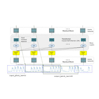
A foundation model for time-series forecasting should adapt to variable context (what we observe) and horizon (what we query the model to forecast) lengths, while having enough capacity to encode all patterns from a large pretraining dataset. Similar to LLMs, we use stacked transformer layers (self-attention and feedforward layers) as the main building blocks for the TimesFM model. In the context of time-series forecasting, we treat a patch (a group of contiguous time-points) as a token that was popularized by a recent long-horizon forecasting work. The task then is to forecast the (i+1)-th patch of time-points given the i-th output at the end of the stacked transformer layers.
However, there are several key differences from language models. Firstly, we need a multilayer perceptron block with residual connections to convert a patch of time-series into a token that can be input to the transformer layers along with positional encodings (PE). For that, we use a residual block similar to our prior work in long-horizon forecasting. Secondly, at the other end, an output token from the stacked transformer can be used to predict a longer length of subsequent time-points than the input patch length, i.e., the output patch length can be larger than the input patch length.
Consider a time-series of length 512 time-points being used to train a TimesFM model with input patch length 32 and output patch length 128. During training, the model is simultaneously trained to use the first 32 time-points to forecast the next 128 time-points, the first 64 time-points to forecast time-points 65 to 192, the first 96 time-points to forecast time-points 97 to 224 and so on. During inference, suppose the model is given a new time-series of length 256 and tasked with forecasting the next 256 time-points into the future. The model will first generate the future predictions for time-points 257 to 384, then condition on the initial 256 length input plus the generated output to generate time-points 385 to 512. On the other hand, if in our model the output patch length was equal to the input patch length of 32 then for the same task we would have to go through eight generation steps instead of just the two above. This increases the chances of more errors accumulating and therefore, in practice, we see that a longer output patch length yields better performance for long-horizon forecasting
TimesFM architecture.
Pretraining data
Just like LLMs get better with more tokens, TimesFM requires a large volume of legitimate time series data to learn and improve. We have spent a great amount of time creating and assessing our training datasets, and the following is what we have found works best:
Synthetic data helps with the basics. Meaningful synthetic time-series data can be generated using statistical models or physical simulations. These basic temporal patterns can teach the model the grammar of time series forecasting.
Real-world data adds real-world flavor. We comb through available public time series datasets, and selectively put together a large corpus of 100 billion time-points. Among these datasets there are Google Trends and Wikipedia Pageviews, which track what people are interested in, and that nicely mirrors trends and patterns in many other real-world time series. This helps TimesFM understand the bigger picture and generalize better when provided with domain-specific contexts not seen during training.
Zero-shot evaluation results
We evaluate TimesFM zero-shot on data not seen during training using popular time-series benchmarks. We observe that TimesFM performs better than most statistical methods like ARIMA, ETS and can match or outperform powerful DL models like DeepAR, PatchTST that have been explicitly trained on the target time-series.
We used the Monash Forecasting Archive to evaluate TimesFM’s out-of-the-box performance. This archive contains tens of thousands of time-series from various domains like traffic, weather, and demand forecasting covering frequencies ranging from few minutes to yearly data. Following existing literature, we inspect the mean absolute error (MAE) appropriately scaled so that it can be averaged across the datasets. We see that zero-shot (ZS) TimesFM is better than most supervised approaches, including recent deep learning models. We also compare TimesFM to GPT-3.5 for forecasting using a specific prompting technique proposed by llmtime(ZS). We demonstrate that TimesFM performs better than llmtime(ZS) despite being orders of magnitude smaller.
Scaled MAE (the lower the better) of TimesFM(ZS) against other supervised and zero-shot approaches on Monash datasets.
Most of the Monash datasets are short or medium horizon, i.e., the prediction length is not too long. We also test TimesFM on popular benchmarks for long horizon forecasting against a recent state-of-the-art baseline PatchTST (and other long-horizon forecasting baselines). In the next figure, we plot the MAE on ETT datasets for the task of predicting 96 and 192 time-points into the future. The metric has been calculated on the last test window of each dataset (as done by the llmtime paper). We see that TimesFM not only surpasses the performance of llmtime(ZS) but also matches that of the supervised PatchTST model explicitly trained on the respective datasets.
Last window MAE (the lower the better) of TimesFM(ZS) against llmtime(ZS) and long-horizon forecasting baselines on ETT datasets.
Conclusion
We train a decoder-only foundation model for time-series forecasting using a large pretraining corpus of 100B real world time-points, the majority of which was search interest time-series data derived from Google Trends and pageviews from Wikipedia. We show that even a relatively small 200M parameter pretrained model that uses our TimesFM architecture displays impressive zero-shot performance on a variety of public benchmarks from different domains and granularities.
Acknowledgements
This work is the result of a collaboration between several individuals across Google Research and Google Cloud, including (in alphabetical order): Abhimanyu Das, Weihao Kong, Andrew Leach, Mike Lawrence, Alex Martin, Rajat Sen, Yang Yang and Yichen Zhou.
Troubleshoot LLMs and Retrieval Augmented Generation with Retrieval and Response Metrics
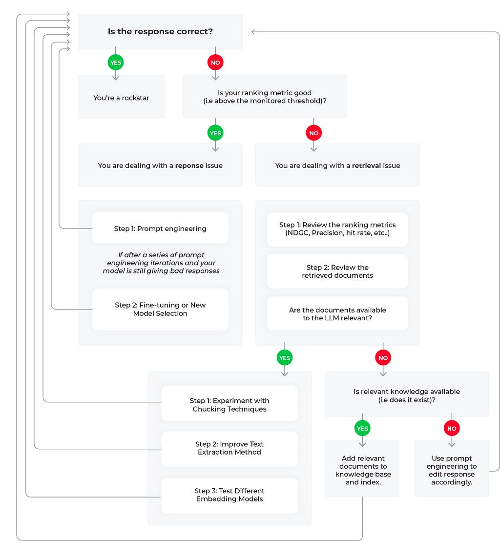
Figure 1: Root Cause Workflows for LLM RAG Applications (flowchart created by author)
If you have been experimenting with large language models (LLMs) for search and retrieval tasks, you have likely come across retrieval augmented generation (RAG) as a technique to add relevant contextual information to LLM generated responses. By connecting an LLM to private data, RAG can enable a better response by feeding relevant data in the context window.
RAG has been shown to be highly effective for complex query answering, knowledge-intensive tasks, and enhancing the precision and relevance of responses for AI models, especially in situations where standalone training data may fall short.
However, these benefits from RAG can only be reaped if you are continuously monitoring your LLM system at common failure points — most notably with response and retrieval evaluation metrics. In this piece we will go through the best workflows for troubleshooting poor retrieval and response metrics.
Troubleshooting Retrieval and Responses
It’s worth remembering that RAG works best when required information is readily available. Whether relevant documents are availablefocuses RAG system evaluations on two critical aspects:
Retrieval Evaluation: To assess the accuracy and relevance of the documents that were retrieved
Response Evaluation: Measure the appropriateness of the response generated by the system when the context was provided
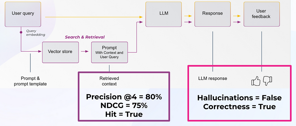
Figure 2: Response Evals and Retrieval Evals in an LLM Application (image by author)
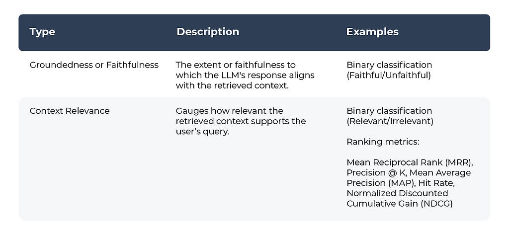
Table 1: Response Evaluation Metrics
Table 1 by author
Table 2: Retrieval Evaluation Metrics
Table 2 by author
Troubleshooting RAG Workflows
Let’s review three potential scenarios to troubleshoot poor LLM performance based on the flow diagram.
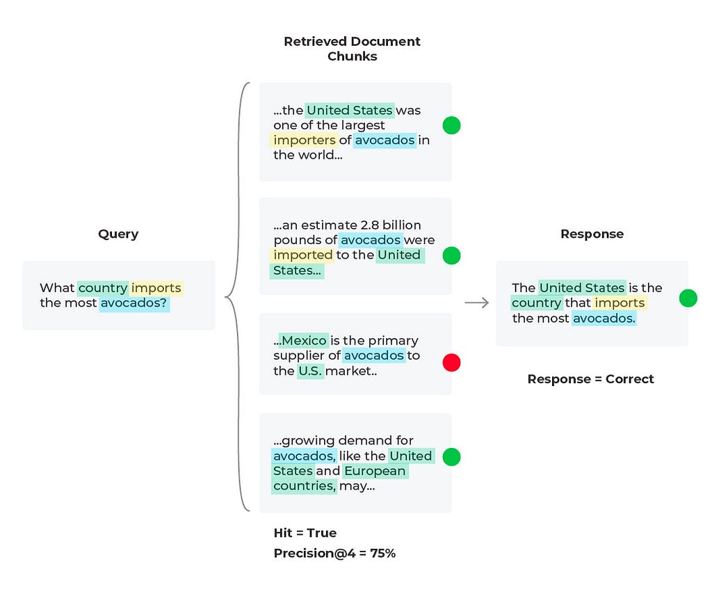
Scenario 1: Good Response, Good Retrieval
Diagram by author
In this scenario everything in the LLM application is acting as expected and we have a good response with a good retrieval. We find our response evaluation is “correct” and our “Hit = True.” Hit is a binary metric, where “True” means the relevant document was retrieved and “False” would mean the relevant document was not retrieved. Note that the aggregate statistic for Hit is the Hit rate (percent of queries that have relevant context).
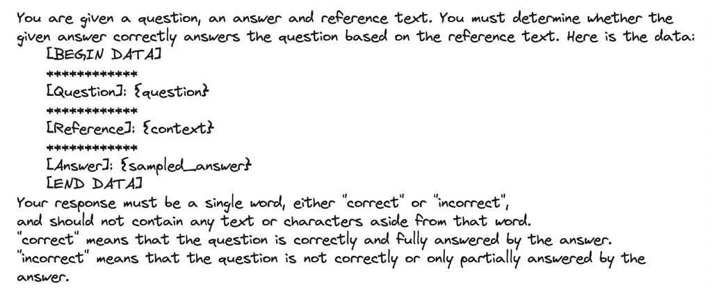
For our response evaluations, correctness is an evaluation metric that can be done simply with a combination of the input (query), output (response), and context as can be seen in Table 1. Several of these evaluation criteria do not require user labeled ground-truth labels since LLMs can also be used to generate labels, scores, and explanations with tools like the OpenAI function calling, below is an example prompt template.
Image by author
These LLM evals can be formatted as numeric, categorical (binary and multi-class) and multi-output (multiple scores or labels) — with categorical-binary being the most commonly used and numeric being the least commonly used.
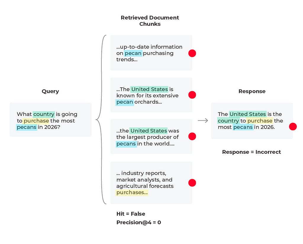
Scenario 2: Bad Response, Bad Retrieval
Diagram by author
In this scenario we find that the response is incorrect and the relevant content was not received. Based on the query we see that the content wasn’t received because there is no solution to the query. The LLM cannot predict future purchases no matter what documents it is supplied. However, the LLM can generate a better response than to hallucinate an answer. Here it would be to experiment with the prompt that is generating the response by simply adding a line to the LLM prompt template of “if relevant content is not provided and no conclusive solution is found, respond that the answer is unknown.” In some cases the correct answer is that the answer does not exist.
Diagram by author
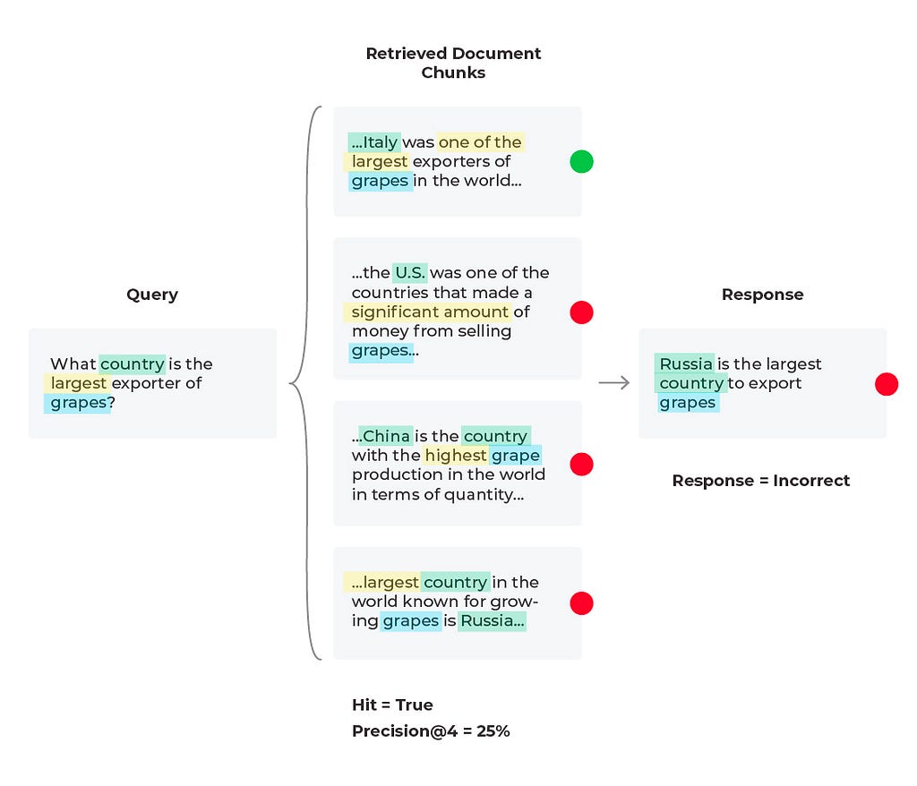
Scenario 3: Bad Response, Mixed Retrieval Metrics
In this third scenario, we see an incorrect response with mixed retrieval metrics (the relevant document was retrieved, but the LLM hallucinated an answer due to being given too much information).
Diagram by author
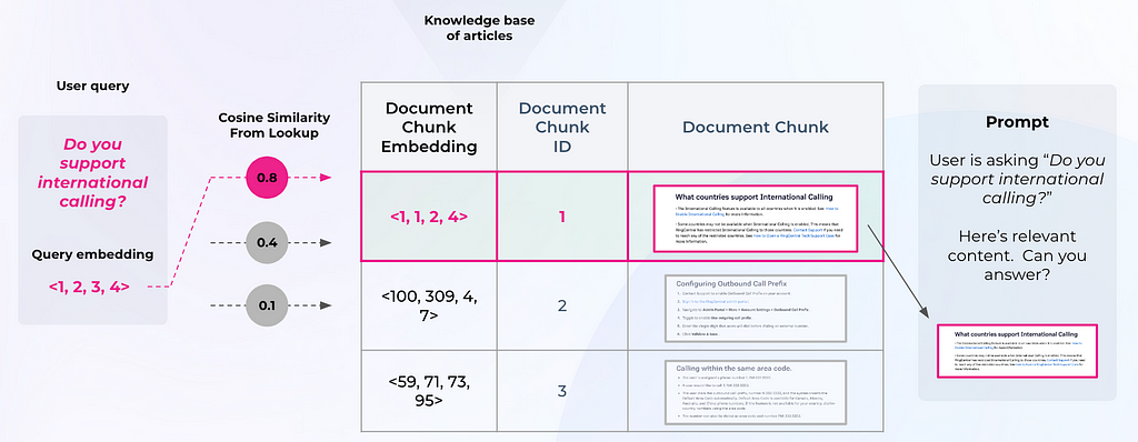
To evaluate an LLM RAG system, you need to both fetch the right context and then generate an appropriate answer. Typically, developers will embed a user query and use it to search a vector database for relevant chunks (see Figure 3). Retrieval performance hinges not only on the returned chunks being semantically similar to the query, but on whether those chunks provide enough relevant information to generate the correct response to the query. Now, you must configure the parameters around your RAG system (type of retrieval, chunk size, and K).
Figure 3: RAG Framework (by author)
Similarly with our last scenario, we can try editing the prompt template or change out the LLM being used to generate responses. Since the relevant content is retrieved during the document retrieval process but isn’t being surfaced by the LLM, this could be a quick solution. Below is an example of a correct response generated from running a revised prompt template (after iterating on prompt variables, LLM parameters, and the prompt template itself).
Diagram by author
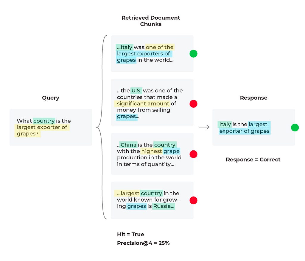
When troubleshooting bad responses with mixed performance metrics, we need to first figure out which retrieval metrics are underperforming. The easiest way of doing this is to implement thresholds and monitors. Once you are alerted to a particular underperforming metric you can resolve with specific workflows. Let’s take nDCG for example. nDCG is used to measure the effectiveness of your top ranked documents and takes into account the position of relevant docs, so if you retrieve your relevant document (Hit = ‘True’), you will want to consider implementing a reranking technique to get the relevant documents closer to the top ranked search results.
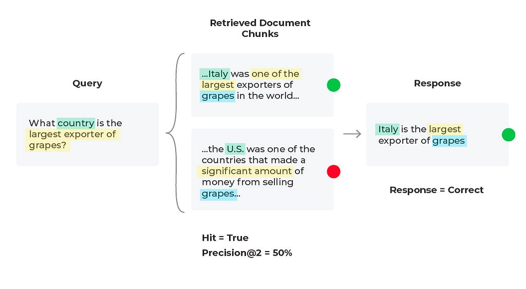
For our current scenario we retrieved a relevant document (Hit = ‘True’), and that document is in the first position, so let’s try and improve the precision (percent relevant documents) up to ‘K’ retrieved documents. Currently our Precision@4 is 25%, but if we used only the first two relevant documents then Precision@2 = 50% since half of the documents are relevant. This change leads to the correct response from the LLM since it is given less information, but more relevant information proportionally.
Diagram by author
Essentially what we were seeing here is a common problem in RAG known as lost in the middle, when your LLM is overwhelmed with too much information that is not always relevant and then is unable to give the best answer possible. From our diagram, we see that adjusting your chunk size is one of the first things many teams do to improve RAG applications but it’s not always intuitive. With context overflow and lost in the middle problems, more documents isn’t always better, and reranking won’t necessarily improve performance. To evaluate which chunk size works best, you need to define an eval benchmark and do a sweep over chunk sizes and top-k values. In addition to experimenting with chunking strategies, testing out different text extraction techniques and embedding methods will also improve overall RAG performance.
Response and Retrieval Evaluation Metrics Summary
The response and retrieval evaluation metrics and approaches in this piece offer a comprehensive way to view an LLM RAG system’s performance, guiding developers and users in understanding its strengths and limitations. By continually evaluating these systems against these metrics, improvements can be made to enhance RAG’s ability to provide accurate, relevant, and timely information.
Additional advanced methods for improving RAG include re-ranking, metadata attachments, testing out different embedding models, testing out different indexing methods, implementing HyDE, implementing keyword search methods, or implementing Cohere document mode (similar to HyDE). Note that while these more advanced methods — like chunking, text extraction, embedding model experimentation — may produce more contextually coherent chunks, these methods are more resource-intensive. Using RAG along with advanced methods can make performance improvements to your LLM system and will continue to do so as long as your retrieval and response metrics are properly monitored and maintained.
Questions? Please reach out to me here or on LinkedIn, X, or Slack!
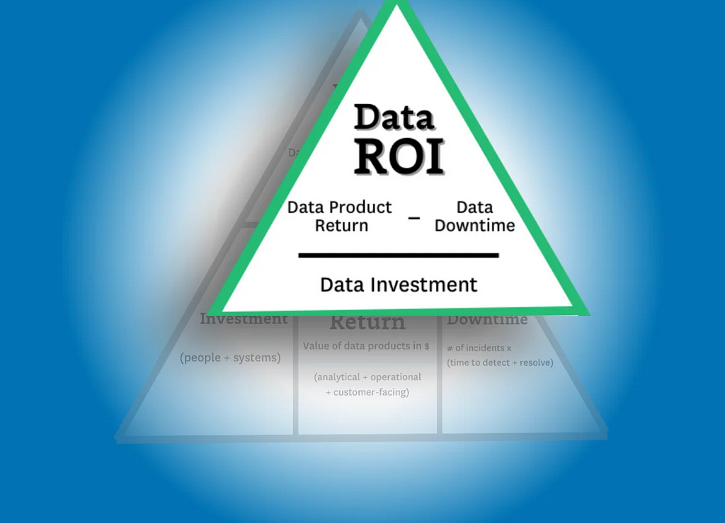
Struggling to articulate the value of your data team? Learn how to calculate your data team’s return with the Data ROI Pyramid.
Image by author.
As recently as a year ago, about half of the data leaders I spoke with felt the business value of their team sold itself. Today, maximizing and measuring data team ROI is near the top of every data leader’s agenda.
Most data team ROI formulas focus on some version of the following calculation:
Lift / investment = ROI.
And while there’s certainly value in its simplicity, it doesn’t capture the full value of the data team. For example, how do you capture the value of:
A customer churn dashboard
A dataset that supports ad hoc queries of engagement behaviors
A migration to a new data stack that supports faster, more scalable compute
Increasing data adoption by 30% as a result of a data quality initiative
It’s not easy! Grizzled data industry veterans who have successfully turned the wild world of customer acquisition funnels into a predictable science start squirming when looking inward.
Over the last six months, I’ve spoken with data leaders and iterated on a variety of ROI formulas, all in an attempt to reach a point that, if not capturing the exact value of a data team, can get us a little closer.
And the result of those conversations has been none other than a brand new data ROI pyramid. Yes, I’m aware of all the great pyramids and conjoined triangles that have come before but this one is different. Sort of.
The goal of this pyramid is aimed squarely at helping data leaders
Get closer to the business
Balance competing priorities
And focus on the right metrics to generate value for their stakeholders.
So, with the preamble out of the way, let’s take it from the top!
Calculating data ROI
Image by author.
As a general rule of thumb, the higher your report in an organization, the fewer and more encompassing your metrics will become. The CEO doesn’t care how many dashboards you support or your data freshness SLA adherence percentage.
They want to know what their investors want to know: “Am I getting a return on my investment?”
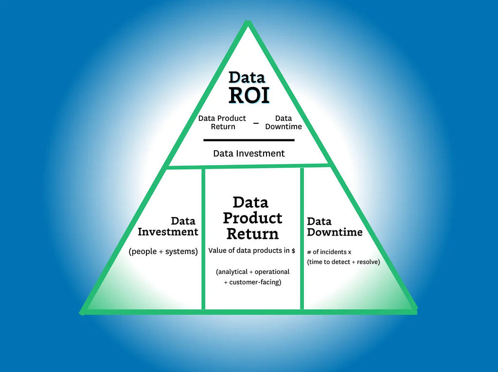
The data ROI pyramid tackles this question with a similar formula to the one in the introduction:
(Data product value — data downtime) / data investment= ROI
…but there are two key differences. The first is the more expansive definition of “data product revenue” (more on that later) and the second is the introduction of data downtime.
The downtime variable is important to include because as more data teams drive higher levels of revenue–via machine learning models, customer-facing apps, data democratization, and other initiatives–the more severe the consequences of downtime becomes in terms of lost time, revenue, and trust.
This also makes reducing data downtime one of the three key strategies for data leaders to increase ROI: you can either increase revenue, you can decrease your investments, or you can reduce your data downtime. And one of those fruits hangs a lot lower than the others.
So, now that we have a framework for calculating ROI, let’s dive deeper into how we identify the variables.
Calculating data investments
Image by author.
The formula is easy — investment = people + solutions.
But it’s also easy to overcomplicate.
Some contracts are annual. Others are not. Some solutions charge based on usage. Others don’t. My recommendation here is to keep this component relatively simple. Stick to an aggregate projection of costs divided evenly across a time period (typically a month or quarter).
Levers to optimize data investments
When it comes to optimizing your data investments, the name of the game is efficiency. To get the most out of your data investments, you need to improve the speed at which those investments deliver value.
Below are three levers you can pull to improve efficiency for your data systems, your data teams, and your data consumers.
System optimization — The cost of almost all modern data solutions is based on usage. The metrics you will want to keep an eye on here are the total number of items that drive these costs (tables, queries, VMs, warehouses, etc) and the outliers at the top (expensive queries) or the bottom (unused tables). A few ways to understand and control system costs could be through assigning ownership for domains, cleaning up unused assets and costly queries, or even consolidating your data stack around central tooling.
Time to build and maintain — The time it takes to build and maintain your key data assets, including data products and machine learning capabilities, is a key lever that measures your data team’s productivity. While larger upfront investments may be required to develop an effective data platform to produce, simplifying the workflows for building and maintaining data pipelines can have a dramatic impact on data team efficiency.
Time to insight (or action) — This lever is focused on the time it takes your data consumers to realize value. In other words, how effectively has the data team enabled your data consumers? Discoverability and self-service can both work to improve time-to-insight for consumers, while micro-batch infrastructures can make that data available at the lowest possible latency for machine learning, analytics, and reporting.
Time spent enabling data self-service is usually well-spent, but the pay-off must be greater than the effort spent to build and maintain it. Image courtesy of Shane Murray.
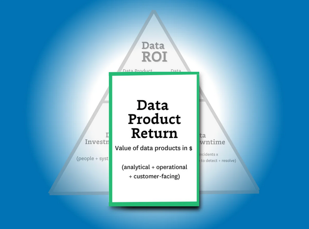
Calculating data product return
Image by author.
Calculating data product return is by far the most complex step in our ROI calculation. That’s because as the data industry continues to advance, the variety and complexity of data product use cases has continued advancing right along with it.
Fortunately, data products can generally be split into one of three primary categories: analytical data products, operational data products, and customer-facing data products. These can exist in the form of dashboards, ML models, experiments leveraging data insights, and — of course — generative AI. While the latter may be a bit more complex to build, genAI is still a data product at its core and its value can still be calculated using the methodologies we’ll outline below.
To really answer this question, the formula for data product return needs to be inclusive of all data team activities, whether they produce value directly (for example revenue generated via a paywall ML model) or indirectly (for example a customer churn dashboard).
The formula I would propose for calculating data product return is this:
Value from Analytical Data Products + Operational Data Products + Customer Facing Data Products = Data Product Return
As you can see, this part of the equation presents the most variables for our ROI calculation. Since this part of the equation is by far the most complicated, we’ll be spending the majority of our time here. So, with that in mind, let’s take a look at each subcategory (or use case) in a bit more detail.
Analytical Data Products
First, let’s dig into the value of the most traditional — and common — data use case: analytics.
Analytical data products are a mix of the critical dashboards, ML models, and experiments conducted and supported by your data team to deliver insights for decision making.
Whether we’re talking about the marketing dashboards or important metrics like customer LTV, analytical data products play a fundamental role in the day-to-day operations of any business. But in the same way that all data products aren’t created equal, the way you’ll calculate their value isn’t either. And, of course, some will be easier to calculate than others.
First, let’s look at experiments:
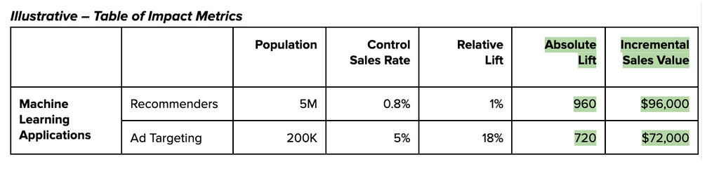
Measuring incremental impact
Measuring absolute impact is one of the simplest ways to understand return from any data product. And calculating the value of an experiment conducted as a result of your data team’s research and analytical insights can be quickly estimated by understanding the delta between test versus control and translating those numbers into dollars earned/saved each month.
For a more conservative approach, you could estimate value by computing the return against a random or average decision to better represent decisions made without support from your data team.
Combining tens or hundreds of these experiments per year will give you a ballpark figure for the incremental value delivered by the experimentation platform and the analytical work surrounding those experiments.
Measuring value-to-stakeholders
But what about dashboards? Rarely are these initiatives so easily measured by a controlled or natural experiment.
To account for these data products, we’ll need to take a more nuanced approach to estimating value. In this case, we’ll be translating qualitative data into something representative by tapping into the consumers themselves.
Believe it or not, your business users and data consumers are actually quite knowledgeable about how valuable your dashboard is (or isn’t) to them. And their responses can be quantified. While this may not seem rigorous enough at first glance, this is actually similar to the process MIT economists used to determine how free services contribute value to the national GDP. For example, they asked respondents how much they would have to be paid not to use Facebook or Google Maps for a year. ($40 to $50 a month for Facebook if you are curious).
For the most important dashboards, data teams can go a step further by creating a benchmark for respondents, like “We estimate the cost of maintaining this dashboard to be about $5,000 last quarter. In your estimation did it add that level of value to your work over that period of time?” For a baseline, here is how our survey of 200 data professionals revealed they judged their data consumers would value their dashboards:
Less than $500k: 5%
500k-1m: 11%
1m-10m: 49%
10m-25m: 32%
25m+: 5%
Customer Facing Lift
Here I’m referring specifically to data that’s customer facing, not the ML models powered by data. This data use case generally comes in two flavors.
The first is when data IS the product. There are a significant number of businesses that ingest, transform, and then sell data to other companies. It could be a data mining company compiling insights from web scraping eCommerce sites or a television manufacturer that sells viewership data to advertisers.
In this case, calculating is pretty straightforward: the revenue of the data product is the revenue of the sale. When you find ways to enrich this data, you make it more valuable and thus increase the sale price.
However, what about cases where data is only part of the product being offered? For example, a point of sale system providing insights back to the merchant on their foot traffic patterns? Or a video player that breaks down views across audience segments by time?
In some cases, the data will be a nice to have. In other cases, it will be a significant factor on customer acquisition and retention. Luckily, data teams have been experimenting and measuring the impact of features on retention for a while now.
I define operational data use cases as activities that MUST take place. Examples would include reporting to the board or an airline re-accommodating passengers of a delayed flight.
If the data systems went down, these activities would still happen, but they would be considerably more painful. An organization may have to manually collect and aggregate data from across the business for its report or passengers may need to go to the customer service desk rather than have an app automatically present their options for re-accommodation.
In these cases the value is typically best determined by the hours saved between the more automated and more painful process. In some situations, alternative impacts such as fine avoidance or poor customer satisfaction could be calculated as well.
You can optimize data product value by increasing how effective it is and the range of its impact. Some broad proxies to measure this across a wide range of use cases and industries are adoption, reach, and velocity.
Adoption and Reach — The more use a data product sees, the more value it can ostensibly provide. So driving improved reach and adoption can also dramatically increase the incremental value your data products will provide.
Velocity — One of the biggest drivers of experimentation value is velocity: how many meaningful experiments can the organization execute over a period of time? More velocity can mean improved productivity, a more mature central platform, and even improved enablement for data consumers.
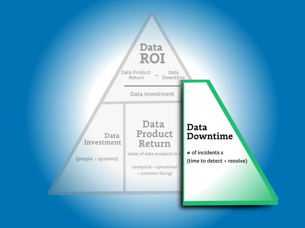
Calculating data downtime
Image by author.
Finally, we need to understand how data downtime impacts ROI.
In other articles, we’ve discussed how to calculate data downtime using your incident and response times. Here’s what that formula looks like:
Number of incidents x (average time to detection + average time to resolution)
This is helpful in measuring how your overall data product reliability is trending. But in this case, we aren’t as interested in the aggregate data downtime or the efficiency of the team (yet).
What we want to find out here is the operational cost for the data downtime of specific data products. To do this, you’ll need data lineage in order to understand the impact a data issue on an upstream table has across various downstream data products.
Since we’ve already calculated the revenue generated from each of our data products, including key dashboards, we can now subtract the operational cost of that downtime from the revenue.
For this component of the ROI calculation, I recommend only focusing on downtime that violates your data SLAs. If a dashboard that’s checked daily has a data freshness issue that only persists for a few hours before being resolved, that downtime is unlikely to have an operational impact on the organization (and your data team shouldn’t be penalized for it).
Levers to minimize data downtime
Improvements in data downtime can have a dramatic impact on your data team’s ROI calculation, especially for use cases where the data is so central to the product offering that data downtime is equivalent to operational downtime.
We’ve covered the metric the CEO cares about and the strategic metrics data leaders should consider. Now let’s talk about the tactical levers your team can pull to maximize your outcomes across these strategic metrics.
SLA Adherence
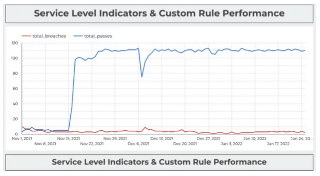
SLA adherence, the amount of time the SLA has been breached divided by the amount of time it has been upheld, can help data teams maintain a granular understanding of how many data quality incidents are having an adverse impact on specific data assets — and what measures to take top protect the value of those products.
Coverage%
Minimizing data downtime can often be directly correlated to how well your data products are covered with monitors and custom tests from raw ingestion to final resulting table. Data pipelines and systems are radically interdependent. Higher coverage percentage typically will translate into better time to detection and resolution.
Status Update%
The teams that are the best at documenting their incident history are almost always the ones with the lowest downtime. High status update percentages encourage a lower time to resolution and can even help prevent incidents by providing better insight into overall data health.
If your data team has a low status update percentage it is either because of alert fatigue or because your team is unable to quickly triage incidents.
Calculating Data ROI Is Hard — But It’s Worth It
While I am under no illusions that calculating the ROI of a data product is either an exact science or a quick win, I will ardently uphold that it’s a worthwhile endeavor — and perhaps most importantly, an achievable destination.
I am also confident there are few activities more existentially critical for data leaders.
By better quantifying and optimizing the data team’s value, we can better earn our colleagues trust and recognition of the value we add to the business. At that point, the sky’s the limit for motivated, well-led data teams.
Posted by Rishabh Tiwari, Pre-doctoral Researcher, and Pradeep Shenoy, Research Scientist, Google Research
Machine learning models in the real world are often trained on limited data that may contain unintended statistical biases. For example, in the CELEBA celebrity image dataset, a disproportionate number of female celebrities have blond hair, leading to classifiers incorrectly predicting “blond” as the hair color for most female faces — here, gender is a spurious feature for predicting hair color. Such unfair biases could have significant consequences in critical applications such as medical diagnosis.
Surprisingly, recent work has also discovered an inherent tendency of deep networks to amplify such statistical biases, through the so-called simplicity bias of deep learning. This bias is the tendency of deep networks to identify weakly predictive features early in the training, and continue to anchor on these features, failing to identify more complex and potentially more accurate features.
With the above in mind, we propose simple and effective fixes to this dual challenge of spurious features and simplicity bias by applying early readouts and feature forgetting. First, in “Using Early Readouts to Mediate Featural Bias in Distillation”, we show that making predictions from early layers of a deep network (referred to as “early readouts”) can automatically signal issues with the quality of the learned representations. In particular, these predictions are more often wrong, and more confidently wrong, when the network is relying on spurious features. We use this erroneous confidence to improve outcomes in model distillation, a setting where a larger “teacher” model guides the training of a smaller “student” model. Then in “Overcoming Simplicity Bias in Deep Networks using a Feature Sieve”, we intervene directly on these indicator signals by making the network “forget” the problematic features and consequently look for better, more predictive features. This substantially improves the model’s ability to generalize to unseen domains compared to previous approaches. Our AI Principles and our Responsible AI practices guide how we research and develop these advanced applications and help us address the challenges posed by statistical biases.
Animation comparing hypothetical responses from two models trained with and without the feature sieve.
Early readouts for debiasing distillation
We first illustrate the diagnostic value of early readouts and their application in debiased distillation, i.e., making sure that the student model inherits the teacher model’s resilience to feature bias through distillation. We start with a standard distillation framework where the student is trained with a mixture of label matching (minimizing the cross-entropy loss between student outputs and the ground-truth labels) and teacher matching (minimizing the KL divergence loss between student and teacher outputs for any given input).
Suppose one trains a linear decoder, i.e., a small auxiliary neural network named as Aux, on top of an intermediate representation of the student model. We refer to the output of this linear decoder as an early readout of the network representation. Our finding is that early readouts make more errors on instances that contain spurious features, and further, the confidence on those errors is higher than the confidence associated with other errors. This suggests that confidence on errors from early readouts is a fairly strong, automated indicator of the model’s dependence on potentially spurious features.
Illustrating the usage of early readouts (i.e., output from the auxiliary layer) in debiasing distillation. Instances that are confidently mispredicted in the early readouts are upweighted in the distillation loss.
We used this signal to modulate the contribution of the teacher in the distillation loss on a per-instance basis, and found significant improvements in the trained student model as a result.
We evaluated our approach on standard benchmark datasets known to contain spurious correlations (Waterbirds, CelebA, CivilComments, MNLI). Each of these datasets contain groupings of data that share an attribute potentially correlated with the label in a spurious manner. As an example, the CelebA dataset mentioned above includes groups such as {blond male, blond female, non-blond male, non-blond female}, with models typically performing the worst on the {non-blond female} group when predicting hair color. Thus, a measure of model performance is its worst group accuracy, i.e., the lowest accuracy among all known groups present in the dataset. We improved the worst group accuracy of student models on all datasets; moreover, we also improved overall accuracy in three of the four datasets, showing that our improvement on any one group does not come at the expense of accuracy on other groups. More details are available in our paper.
Comparison of Worst Group Accuracies of different distillation techniques relative to that of the Teacher model. Our method outperforms other methods on all datasets.
Overcoming simplicity bias with a feature sieve
In a second, closely related project, we intervene directly on the information provided by early readouts, to improve feature learning and generalization. The workflow alternates between identifying problematic features and erasing identified features from the network. Our primary hypothesis is that early features are more prone to simplicity bias, and that by erasing (“sieving”) these features, we allow richer feature representations to be learned.
Training workflow with feature sieve. We alternate between identifying problematic features (using training iteration) and erasing them from the network (using forgetting iteration).
We describe the identification and erasure steps in more detail:
Identifying simple features: We train the primary model and the readout model (AUX above) in conventional fashion via forward- and back-propagation. Note that feedback from the auxiliary layer does not back-propagate to the main network. This is to force the auxiliary layer to learn from already-available features rather than create or reinforce them in the main network.
Applying the feature sieve: We aim to erase the identified features in the early layers of the neural network with the use of a novel forgetting loss, Lf , which is simply the cross-entropy between the readout and a uniform distribution over labels. Essentially, all information that leads to nontrivial readouts are erased from the primary network. In this step, the auxiliary network and upper layers of the main network are kept unchanged.
We can control specifically how the feature sieve is applied to a given dataset through a small number of configuration parameters. By changing the position and complexity of the auxiliary network, we control the complexity of the identified- and erased features. By modifying the mixing of learning and forgetting steps, we control the degree to which the model is challenged to learn more complex features. These choices, which are dataset-dependent, are made via hyperparameter search to maximize validation accuracy, a standard measure of generalization. Since we include “no-forgetting” (i.e., the baseline model) in the search space, we expect to find settings that are at least as good as the baseline.
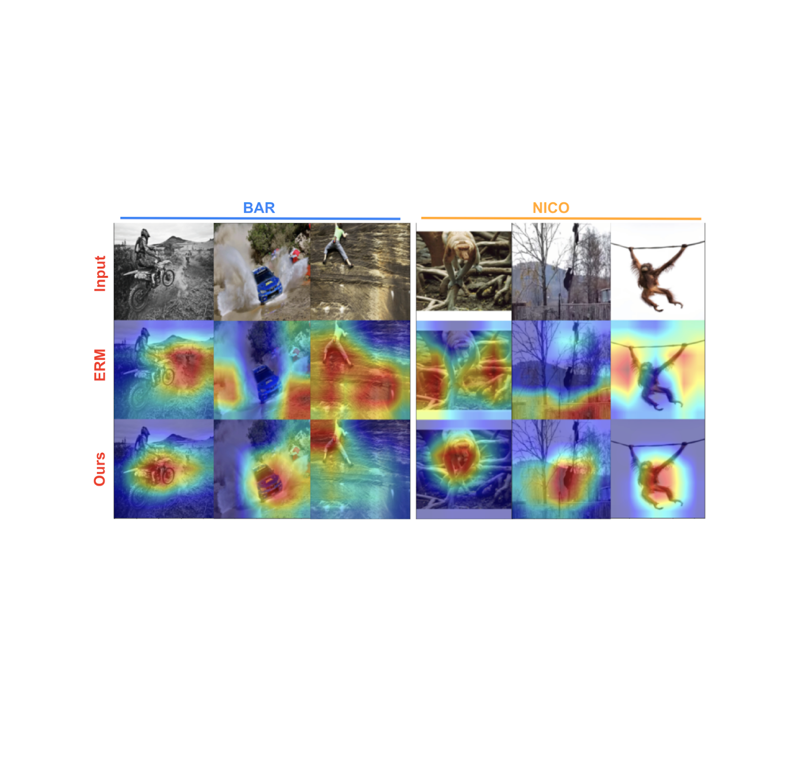
Below we show features learned by the baseline model (middle row) and our model (bottom row) on two benchmark datasets — biased activity recognition (BAR) and animal categorization (NICO). Feature importance was estimated using post-hoc gradient-based importance scoring (GRAD-CAM), with the orange-red end of the spectrum indicating high importance, while green-blue indicates low importance. Shown below, our trained models focus on the primary object of interest, whereas the baseline model tends to focus on background features that are simpler and spuriously correlated with the label.
Feature importance scoring using GRAD-CAM on activity recognition (BAR) and animal categorization (NICO) generalization benchmarks. Our approach (last row) focuses on the relevant objects in the image, whereas the baseline (ERM; middle row) relies on background features that are spuriously correlated with the label.
Through this ability to learn better, generalizable features, we show substantial gains over a range of relevant baselines on real-world spurious feature benchmark datasets: BAR, CelebA Hair, NICO and ImagenetA, by margins up to 11% (see figure below). More details are available in our paper.
Our feature sieve method improves accuracy by significant margins relative to the nearest baseline for a range of feature generalization benchmark datasets.
Conclusion
We hope that our work on early readouts and their use in feature sieving for generalization will both spur the development of a new class of adversarial feature learning approaches and help improve the generalization capability and robustness of deep learning systems.
Acknowledgements
The work on applying early readouts to debiasing distillation was conducted in collaboration with our academic partners Durga Sivasubramanian, Anmol Reddy and Prof. Ganesh Ramakrishnan at IIT Bombay. We extend our sincere gratitude to Praneeth Netrapalli and Anshul Nasery for their feedback and recommendations. We are also grateful to Nishant Jain, Shreyas Havaldar, Rachit Bansal, Kartikeya Badola, Amandeep Kaur and the whole cohort of pre-doctoral researchers at Google Research India for taking part in research discussions. Special thanks to Tom Small for creating the animation used in this post.
One of the most useful application patterns for generative AI workloads is Retrieval Augmented Generation (RAG). In the RAG pattern, we find pieces of reference content related to an input prompt by performing similarity searches on embeddings. Embeddings capture the information content in bodies of text, allowing natural language processing (NLP) models to work with […]
Imagine a scenario where you just started an A/B test that will be running for the next two weeks. However, after just a day or two, it is becoming increasingly clear that version A is working better for certain types of users, whereas version B is working better for another set of users. You think to yourself: Perhaps I should re-route the traffic such that users are getting more of the version that is benefiting them more, and less of the other version. Is there a principled way to achieve this?
Contextual bandits are a class of one-step reinforcement learning algorithms specifically designed for such treatment personalization problems where we would like to dynamically adjust traffic based on which treatment is working for whom. Despite being incredibly powerful in what they can achieve, they are one of the lesser known methods in Data Science, and I hope that this post will give you a comprehensive introduction to this amazing topic. Without further ado, let’s dive right in!
2. When To Use Contextual Bandits
If you are just getting started with contextual bandits, it can be confusing to understand how contextual bandits are related to other more widely known methods such as A/B testing, and why you might want to use contextual bandits instead of those other methods. Therefore, we start our journey by discussing the similarities and differences between contextual bandits and related methods.
2.1. Contextual Bandit vs Multi-Armed Bandit vs A/B Testing
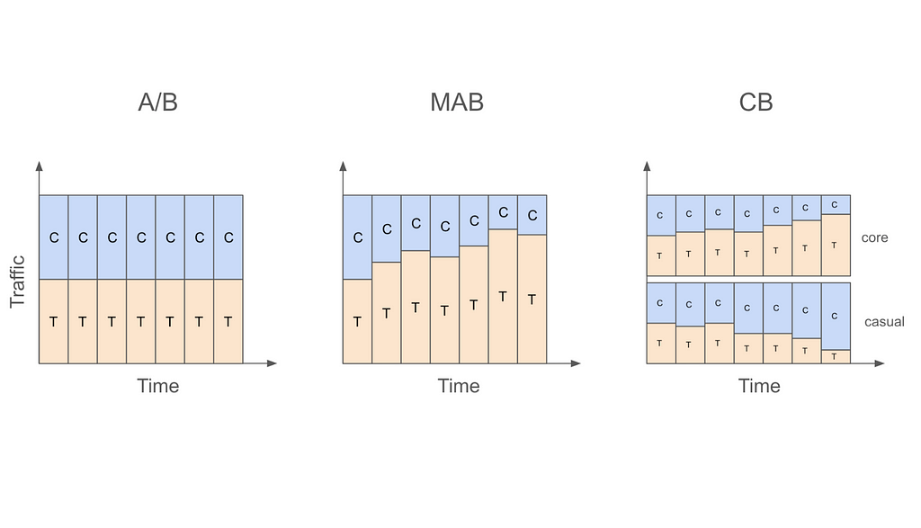
Let us start with the most basic A/B testing setting that allocates traffic into treatment and control in a static fashion. For example, a data scientist might decide to run an A/B test for two weeks with 50% of traffic going to treatment and 50% going to control. What this means is that regardless of whether we are on the first day of the test or the last, we will be assigning users to control or treatment with 50% probability.
On the other hand, if the data scientist were to use a multi-armed bandit (MAB) instead of an A/B test in this case, then traffic will be allocated to treatment and control in a dynamic fashion. In other words, traffic allocations in a MAB will change as days go by. For example, if the algorithm decides that treatment is doing better than control on the first day, the traffic allocation can change from 50% treatment and 50% control to 60% treatment vs 40% control on the second day, and so on.
Despite allocating traffic dynamically, MAB ignores an important fact, which is that not all users are the same. This means that a treatment that is working for one type of user might not work for another. For example, it might be the case that while treatment is working better for core users, control is actually better for casual users. In this case, even if treatment is better overall, we can actually get more value from our application if we assign more core users to treatment and more casual users to control.
This is exactly where contextual bandits (CB) come in. While MAB simply looks at whether treatment or control is doing better overall, CB focuses on whether treatment or control is doing better for a user with a given set of characteristics. The “context” in contextual bandits precisely refers to these user characteristics and is what differentiates it from MAB. For example, CB might decide to increase treatment allocation to 60% for core users but decrease treatment allocation to 40% for casual users after observing first day’s data. In other words, CB will dynamically update traffic allocation taking user characteristics (core vs casual in this example) into account.
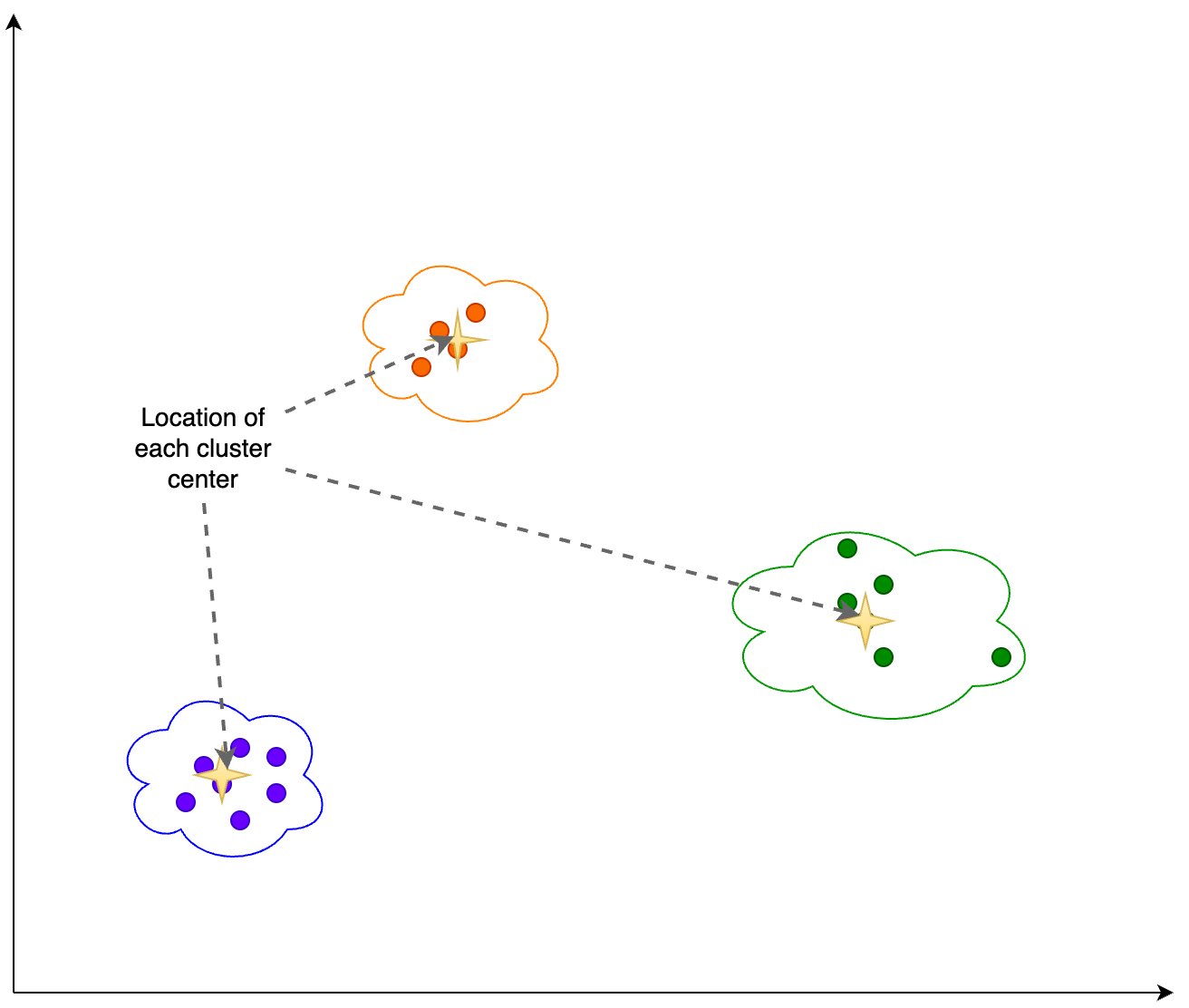
The following table summarizes the key differences between A/B testing, MAB, and CB, and the figure that follows visualizes these ideas.
Table 1: Differences Between A/B Testing, MAB, and CB
Figure 1: Traffic Allocations in A/B Testing, MAB, and CB
2.2. Contextual Bandit vs Multiple MABs
At this point, you might be tempted to think that CB is nothing more than a set of multiple MABs running together. In fact, when the context we are interested in is a small one (e.g., we are only interested in whether a user is a core user or a casual user), we can simply run one MAB for core users and another MAB for casual users. However, as the context gets large (core vs casual, age, country, time since last active, etc.) it becomes impractical to run a separate MAB for each unique context value.
The real value of CB emerges in this case through the use of models to describe the relationship of the experimental conditions in different contexts to our outcome of interest (e.g., conversion). As opposed to enumerating through each context value and treating them independently, the use of models allows us to share information from different contexts and makes it possible to handle large context spaces. This idea of a model will be discussed at several different points in this post, so keep on reading to learn more.
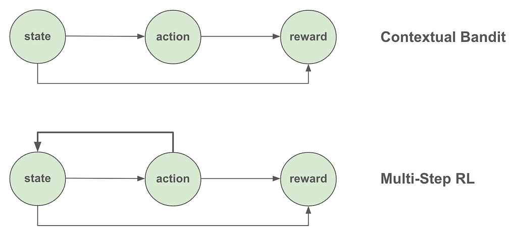
2.3. Contextual Bandit vs Multi-Step Reinforcement Learning
The introduction referred to CB as a class of one-step reinforcement learning (RL) algorithms. So, what exactly is the difference between one-step and multi-step RL? And what makes CB one-step? The fundamental difference between CB and multi-step RL is that in CB we assume the actions the algorithm takes (e.g., serve treatment or control to a specific user) don’t affect the future states of the overall system. In other words, the state (or “context” as is more appropriately called in CB) affects what action we take, but that action we took does not in turn impact or change the state. The following figure summarizes this distinction.
A few examples should make this distinction clearer. Let’s say that we are building a system to decide what ads to show to users based on their age. We would expect that users from different age groups may find different ads more relevant to them, which means that a user’s age should affect what ads we should show them. However, the ad we showed them doesn’t in turn affect their age, so the one-step assumption of CB seems to hold. However, if we move one step further and find out that serving expensive ads deplete our inventory (and limit which ads we can serve in the future) or that the ad we show today affect whether the user will visit our site again, then the one-step assumption is indirectly inviolated, so we may want to consider developing a full-blown RL system instead.
A note of caution though: While multi-step reinforcement learning is more flexible compared to contextual bandits, it’s also more complicated to implement. So, if the problem at hand can be accurately framed as a one-step problem (even though it looks like a multi-step problem at first glance), contextual bandits could be the more practical approach.
2.4. Contextual Bandit vs Uplift Modeling
Before moving on to discussing different CB algorithms, I would also like to briefly touch upon the connection between CB and uplift modeling. An uplift model is usually built on top of A/B test data to discover the relationship between the treatment effect (uplift) and user characteristics. The results from such a model can then be used to personalize treatments in the future. For example, if the uplift model discovers that certain users are more likely to benefit from a treatment, then only those types of users might be given the treatment in the future.
Given this description of uplift modeling, it should be clear that both CB and uplift modeling are solutions to the personalization problem. The key difference between them is that CB approaches this problem in a more dynamic way in the sense that personalization happens on-the-fly instead of waiting for results from an A/B test. At a conceptual level, CB can very loosely be thought of as A/B testing and uplift modeling happening concurrently instead of sequentially. Given the focus of this post, I won’t be discussing uplift modeling further, but there are several great resources to learn more about it such as [1].
3. Exploration and Exploitation in Contextual Bandits
Above we discussed how CB dynamically allocates traffic depending on whether treatment or control is doing better for a given group of users at a given point in time. This raises an important question: How aggressive do we want to be when we are making these traffic allocation changes? For example, if after just one day of data we decide that treatment is working better for users from the US, should we completely stop serving control to US users?
I’m sure most of you would agree that this would be a bad idea, and you would be correct. The main problem with changing traffic allocations this aggressively is that making inferences based on insufficient amounts of data can lead to erroneous conclusions. For example, it might be that the first day of data we gathered is actually not representative of dormant users and that in reality control is better for them. If we stop serving control to US users after the first day, we will never be able to learn this correct relationship.
A better approach to dynamically updating traffic allocations is striking the right balance between exploitation (serve the best experimental condition based on the data so far) and exploration (continue to serve other experimental conditions as well). Continuing with the previous example, if data from the first day indicate that treatment is better for US users, we can serve treatment to these users with an increased probability the next day while still allocating a reduced but non-zero fraction to control.
There are numerous exploration strategies used in CB (and MAB) as well as several variations of them that try to strike this right balance between exploration and exploitation. Three popular strategies include ε-greedy, upper confidence bound, and Thompson sampling.
3.1. ε-greedy
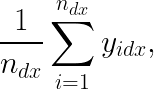
In this strategy, we first decide which experimental condition is doing better for a given group of users at a given point in time. The simplest way to do this is by comparing the average target values (y) for each experimental condition for these users. More formally, we can decide the “winning” condition for a group of users by finding the condition d that has the higher value for
where n_dx is the number of samples we have so far from users in condition d with context x, and y_idx is the target value for a given sample i in condition d with context x.
After deciding which experimental condition is currently “best” for these users, we serve them that condition with 1-ε probability (where ε is usually a small number such as 0.05) and serve a random experimental condition with probability ε. In reality, we might want to dynamically update our ε such that it is large at the beginning of the experiment (when more exploration is needed) and gradually gets smaller as we collect more and more data.
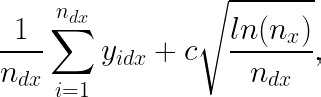
Additionally, context X might be high-dimensional (country, gender, platform, tenure, etc.) so we might want to use a model to get these y estimates to deal with the curse of dimensionality. Formally, the condition to serve can be decided by finding the condition d that has the higher value for
where x^T is an m-dimensional row-vector of context values and θ_d is an m-dimensional column-vector of learnable parameters associated with condition d.
3.2. Upper Confidence Bound (UCB)
This strategy decides the next condition to serve by looking at not only which condition has a higher y estimate but also our precision of (or confidence in) that estimate. In a simple MAB setting, precision can be thought to be a function of how many times a given condition has already been served so far. In particular, a condition that (i) has a high average y (so it makes sense to exploit) or (ii) has not yet been served many times (so it needs more exploration) is more likely to be served next.
We can generalize this idea to the CB setting by keeping track of how many times different conditions are served in different contexts. Assuming a simple setting with a low-dimensional context X such that CB can be thought of as just multiple MABs running together, we can select the next condition to serve based on which condition d has the higher value for
where c is some constant (to be selected based on how much emphasis we want to put on the precision of our estimate when exploring) and n_x is the number of times context x is seen so far.
However, in most cases, the context X will be high-dimensional, which means that just like in the ε-greedy case, we would need to make use of a model. In this setting, a condition d can be served next if it has the higher value for
where SE(.) is the standard error of our estimate (or more generally a metric that quantifies our current level of confidence in that estimate).
Note that there are several versions of UCB, so you will likely come across different formulas. A popular UCB method is LinUCB that formalizes the problem in a linear model framework (e.g., [2]).
3.3. Thompson Sampling
The third and final exploration strategy to be discussed is Thompson sampling, which is a Bayesian approach to solving the exploration-exploitation dilemma. Here, we have a model f(D, X; Θ) that returns predicted y values given experimental condition D, context X, and some set of learnable parameters Θ. This function gives us access to posterior distributions of expected y values for any condition-context pair, thus allowing us to choose the next condition to serve according to the probability that it yields the highest expected y given context. Thompson sampling naturally balances exploration and exploitation as we are sampling from the posterior and updating our model based on the observations. To make these ideas more concrete, here are the steps involved in Thompson sampling:
In practice, instead of having a single function we can also use a different function for each experimental condition (e.g., evaluate both f_c(X; Θ_c) and f_t(X; Θ_t) and then select the condition with the higher value). Furthermore, the update step usually takes place not after each sample but rather after seeing a batch of samples. For more details on Thompson sampling, you can refer to [3][4].
4. Contextual Bandit Algorithm Steps
The previous section (especially the part on Thompson sampling) should already give you a pretty good sense of the steps involved in a CB algorithm. However, for the sake of completeness, here is a step-by-step description of a standard CB algorithm:
A new data point arrives with context X (e.g., a core user with an iOS device in the US).
Given this data point and the exploration strategy chosen (e.g., ε-greedy), the algorithm decides on a condition to serve this user (e.g., treatment or control).
After the condition is served, we observe the outcome y (e.g., whether the user made a purchase or not).
Update (or fully retrain) the model used in Step 2 after seeing the new data. (As mentioned previously, we usually make an update not after every sample but after seeing a batch of samples to ensure that updates are less noisy.)
Repeat.
5. Offline Policy Evaluation in Contextual Bandits
So far we have only discussed how to implement a CB algorithm as new data come in. An equally important topic to cover is how to evaluate a CB algorithm using old (or logged) data. This is called offline evaluation or offline policy evaluation (OPE).
5.1. OPE Using Causal Inference Methods
One way to do OPE is using well-known causal inference techniques such as Inverse Propensity Scoring (IPS) or the Doubly Robust (DR) method. Causal inference is appropriate here because we are essentially trying to estimate the counterfactual of what would have happened if a different policy served a different condition to a user. There is already a great Medium article on this topic [5], so here I will only briefly summarize the main idea from that piece and adapt it to our discussion.
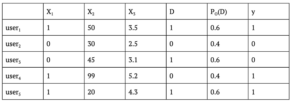
Taking IPS as an example, doing OPE usually requires us to know not only (i) the probability of assigning a given condition to a sample using our new CB algorithm but also (ii) the probability with which a given condition was assigned to a sample in the logged data. Take the following hypothetical logged data with X_1-X_3 being context, D being the experimental condition, P_O(D) being the probability of assigning D to that user, and y being the outcome.
Table 2: Example Logged Data From An A/B Test
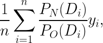
As you can see, in this example P_O(D) is always 0.6 for D=1 and 0.4 for D=0 regardless of the context, so the logged data can be assumed to come from an A/B test that assigns treatment with probability 0.6. Now, if we want to test how a CB algorithm would have performed had we assigned conditions using a CB algorithm rather than a simple A/B test, we can use the following formula to get the IPS estimate of the cumulative y for CB
where n is the number of samples in the logged data (which is 5 here) and P_N(D_i) is the probability of serving the logged D for user_i had we used the new CB algorithm instead (this probability will depend on the specific algorithm being evaluated).
Once we have this estimate, we can compare that to the observed cumulative y from the old A/B test (which is 1+0+0+1+1=3 here) to decide if the CB would have yielded a higher cumulative y.
For more information on OPE using causal inference methods, please refer to the article linked at the beginning of the section. The article also links to a nice GitHub repo with lots of OPE implementations.
A side note here is that this section discussed causal inference methods only as a technique used in OPE. However, in reality, one can also apply them while the CB algorithm is being run so as to “debias” the training data that the algorithm collects along the way. The reason why we might want to apply methods such as IPS to our training data is that the CB policy that generates this data is a non-uniform random policy by definition, so estimating causal effects from it to decide what action to take would benefit from using causal inference methods. If you would like to learn more about debiasing, please refer to [6].
5.2. OPE Using Sampling Methods
Another way to do OPE is through the use of sampling methods. In particular, a very simple replay method [7] can be used to evaluate a CB algorithm (or any other algorithm for that matter) using logged data from a randomized policy such as an A/B test. In its simplest form (where we assume a uniform random logging policy), the method works as follows:
Sample the next user with context X from the logged data.
Decide what condition to assign to that user using the new CB algorithm.
If the selected condition matches the actual condition in the logged data, then add the observed y to the cumulative y counter. If it doesn’t match, ignore the sample.
Repeat until all samples are considered.
If the logging policy doesn’t assign treatments uniformly at random, then the method needs to be slightly modified. One modification that the authors themselves mention is to use rejection sampling (e.g., [8]) whereby we would accept samples from the majority treatment less often compared to the minority treatment in Step 3. Alternatively, we could consider dividing the observed y by the propensity in Step 3 to similarly “down-weight” the more frequent treatment and “up-weight” the less frequent one.
In the next section, I employ an even simpler method in my evaluation that uses up- and down-sampling with bootstrap to transform the original non-uniform data into a uniform one and then apply the method as it is.
6. Contextual Bandit in Action
To demonstrate contextual bandits in action, I put together a notebook that generates a simulated dataset and compares the cumulative y (or “reward”) estimates for new A/B, MAB, and CB policies evaluated on this dataset. Many parts of the code in this notebook are taken from the Contextual Bandits chapter of an amazing book on Reinforcement Learning [9] (highly recommended if you would like to dig deeper into Reinforcement Learning using Python) and two great posts by James LeDoux [10][11] and adapted to the setting we are discussing here.
The setup is very simple: The original data we have comes from an A/B test that assigned treatment to users with probability 0.75 (so not uniformly at random). Using this randomized logged data, we would like to evaluate and compare the following three policies based on their cumulative y:
A new A/B policy that randomly assigns treatment to users with probability 0.4.
A MAB policy that decides what treatment to assign next using an ε-greedy policy that doesn’t take context X into account.
A CB policy that decides what treatment to assign next using an ε-greedy policy that takes context X into account.
I modified the original method described in the Li et al. paper such that instead of directly sampling from the simulated data (which is 75% treatment and only 25% control in my example), I first down-sample treatment cases and up-sample control cases (both with replacement) to get a new dataset that is exactly 50% treatment and 50% control.
The reason why I start with a dataset that is not 50% treatment and 50% control is to show that even if the original data doesn’t come from a policy that assigns treatment and control uniformly at random, we can still work with that data to do offline evaluation after doing up- and/or down-sampling to massage it into a 50/50% dataset. As mentioned in the previous section, the logic behind up- and down-sampling is similar to rejection sampling and the related idea of dividing the observed y by the propensity.
The following figure compares the three policies described above (A/B vs MAB vs CB) in terms of their cumulative y values.
Figure 3: Cumulative Reward Comparison
As can be seen in this figure, cumulative y increases fastest for CB and slowest for A/B with MAB somewhere in between. While this result is based on a simulated dataset, the patterns observed here can still be generalized. The reason why A/B testing isn’t able to get a high cumulative y is because it isn’t changing the 60/40% allocation at all even after seeing sufficient evidence that treatment is better than control overall. On the other hand, while MAB is able to dynamically update this traffic allocation, it is still performing worse than CB because it isn’t personalizing the treatment vs control assignment based on the context X being observed. Finally, CB is both dynamically changing the traffic allocation and also personalizing the treatment, hence the superior performance.
7. Conclusion
Congratulations on making it to the end of this fairly long post! We covered a lot of ground related to contextual bandits in this post, and I hope that you leave this page with an appreciation of the usefulness of this fascinating method for online experimentation, especially when treatments need to be personalized.
If you are interested in learning more about contextual bandits (or want to go a step further into multi-step reinforcement learning), I highly recommend the book Mastering Reinforcement Learning with Python by E. Bilgin. The Contextual Bandit chapter of this book was what finally gave me the “aha!” moment in understanding this topic, and I kept on reading to learn more about RL in general. As far as offline policy evaluation is concerned, I highly recommend the posts by E. Conti and J. LeDoux, both of which provide great explanations of the techniques involved and provide code examples. Regarding debiasing in contextual bandits, the paper by A. Bietti, A. Agarwal, and J. Langford provides a great overview of the techniques involved. Finally, while this post exclusively focused on using regression models when building contextual bandits, there is an alternative approach called cost-sensitive classification, which you can start learning by checking out these lecture notes by A. Agarwal and S. Kakade [12].
Have fun building contextual bandits!
8. Acknowledgements
I would like to thank Colin Dickens for introducing me to contextual bandits as well as providing valuable feedback on this post, Xinyi Zhang for all her helpful feedback throughout the writing, Jiaqi Gu for a fruitful conversation on sampling methods, and Dennis Feehan for encouraging me to take the time to write this piece.
Unless otherwise noted, all images are by the author.
Inspired by an in-depth Medium article [1] with a case study on identifying bank customer segments with high churn reduction potential, this story explores a similar challenge through the lens of subgroup discovery methods [2]. Intrigued by the parallels, I applied a subgroup discovery approach to the same dataset and uncovered a segment with a 35% higher churn reduction potential — a significant improvement over what was previously reported. This story will take you through each step of the process, including building the methodology from the ground up. At the end of this journey, you’ll gain:
A clear understanding of the Patient Rule Induction Method (PRIM), a mature yet powerful subgroup discovery technique.
The skills to apply PRIM to your datasets and tailor it to your specific needs.
The complete code for PRIM and the experiment is on GitHub [3].
Patient Rule Induction Method
For the experiment, I’ve chosen my favorite subgroup discovery method: PRIM [4]. Despite its long presence in the field, PRIM has a unique mix of properties that make it very versatile:
Numerical data handling: PRIM easily handles numerical data without the need for binning. Unlike typical methods that discretize variables (e.g., categorizing age into predefined groups such as 45–54 years), PRIM overcomes this limitation. For example, it can identify more nuanced criteria such as age > 37.
Intelligent categorical data processing: PRIM can discover complex segments within categorical data. It can go beyond simple classifications such as country = Germany to more complex definitions such as country not in {France}.
Simplicity: While traditional subgroup discovery methods are often burdened with multiple parameters, PRIM is refreshingly simple. It relies primarily on a single, unambiguous peeling parameter: the proportion of points removed from a candidate segment in each iteration.
Efficiency: Being a heuristic approach, PRIM is remarkably fast. Despite its large search space, segment identification is typically resolved in milliseconds.
Interactivity and control: PRIM enables interactive analysis. Users can balance segment size against potential impact by examining a series of “nested” segments and selecting the most appropriate one. It also supports incremental segment discovery by removing already segmented data.
Flexibility: The flexibility of the method extends to the optimization function it is designed to enhance. This function isn’t limited to a single variable. For example, PRIM can identify segments where the correlation between two variables is significantly different from their correlation in the entire data set.
In summary, PRIM’s straightforward logic not only makes it easy to implement, but also allows for customization.
PRIM algorithm
PRIM works through two distinct phases: peeling and pasting. Peeling starts from a segment encompassing the entire dataset and gradually shrinks it while optimizing its quality. Pasting works similarly, but in the opposite direction — it tries to expand the selected candidate segment without quality loss. In our previous experiments [5], we observed that the pasting phase typically contributes minimally to the output quality. Therefore, I will focus on the peeling phase. The underlying logic of the peeling phase is as follows:
1. Initialize:
   - Set the peeling parameter (usually 0.05)
   - Set the initial box (segment) to encompass the entire data space.
   - Define the target quality function (e.g., a potential churn reduction).

2. While the stopping criterion is not met:
   - For each dimension of the data space:
     * Identify a small portion (defined by a peeling parameter)
       of the data to remove that maximizes quality of remaining data
   - Update the box by removing the identified portion from
     the current box.
   - Update the dataset by removing the data points that fall outside
     the new box.

3. End when the stopping criterion is met
   (e.g., after a certain number of iterations
   or minimum number of data points remaining).

4. Return the final box and all the preceding boxes as candidate segments.
In this pseudo-code:
box refers to the current segment of the data.
The target quality function is typically some statistic of the response variable (mean, median, etc) that we want to maximize or minimize.
The peeling parameter determines the proportion of data points to be removed in each iteration. It is usually set to a small value, such as 0.05, hence the word “patient” in the method’s name.
The stopping criterion ensures that enough data points remain for analysis.
Consider simple examples of how PRIM handles numeric and categorical variables:
Numeric variables: Imagine you have a numeric variable such as age. In each step of the peeling phase, PRIM looks at the range of that variable (say, age from 18 to 80). PRIM then “peels off” a portion of that range from either end, as defined by the peeling parameter. For example, it might remove ages 75 to 80 because doing so improves the target quality function in the remaining data (e.g., increasing the churn reduction potential). The animation below shows PRIM finding an interesting segment (with a high proportion of orange squares) in a 2D numeric dataset.
PRIM at work on a 2D numerical data set. Image by the author
Categorical nominal variables: Now consider a categorical nominal variable such as country, with categories such as Germany, France, and Spain. In the peeling phase, PRIM evaluates each category based on how well it improves the target quality function. It then removes the least promising category. For example, if removing “Germany” results in a subset where the target quality function is improved (such as a higher potential churn reduction), then all data points with “Germany” are “peeled”. Note that the peeling parameter has no effect on the processing of categorical data, which can cause undesired effects in some cases, as I will discuss and provide a simple remedy (in section “Better segments via enforced ‘patience’”).
Categorical ordinal variables: For ordinal variables, disjoint intervals in segment descriptions can sometimes be less intuitive. Consider an education variable with levels such as primary, secondary, vocational, bachelor, and graduate. Finding a rule like education in {primary, bachelor} may not fit well with the ordinal nature of the data because it combines non-adjacent categories. For those looking for a more coherent segmentation, such as education > secondary, that respects the natural order of the variable, using an ordinal encoding can be a useful workaround. For more insight into categorical encoding, you may find my earlier post [6] helpful, as it navigates you to the necessary information.
Experiment: Churn for bank customers
Now everything is ready to start the experiment. Following the Medium article on identifying unique data segments [1], I will apply the PRIM method to the Churn for Bank Customers [7] dataset from Kaggle, available under the CC0: Public Domain license. I will also adopt the target quality function from the article:
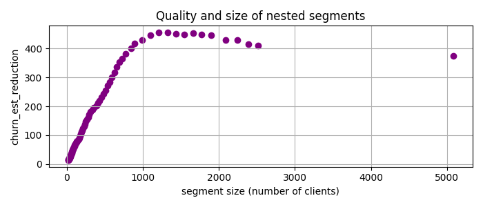
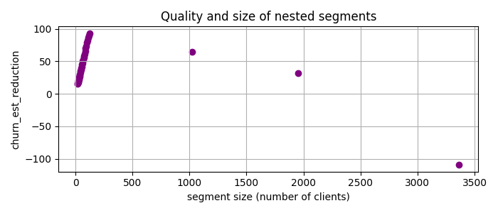
That is, I will look for the segments with many customers where the churn rate is much higher than the baseline, which is the average churn rate in the entire dataset. So I use PRIM, which gives me a set of nested candidate segments, and plot the churn_est_reduction against the number of clients.
Image by the author
The highest quality, churn_est_reduction = 457 is achieved for the 11th candidate segment with the description num_of_products < 2, is_active_member < 1, age > 37. This is quite an improvement over the previously reported maximum churn_est_reduction = 410 in [1]. Comparing the segment descriptions, I suspect that the main reason for this improvement is PRIM’s ability to handle numeric variables.
Better segments via enforced ‘patience’
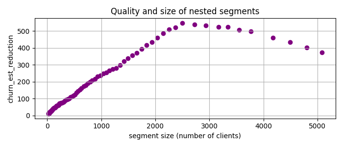
Something suspicious is going on in the previous plot. By its nature, PRIM is expected to be “patient”, i.e. to reduce the segment size only a little bit at each iteration. However, the second candidate segment is twice as small as the previous one — PRIM has cut off half the data at once. The reason for this is the low cardinality of some features, which is often the case with categorical or indicator variables. For example, is_active_member only takes the values 0 or 1. PRIM can only cut off large chunks of data for such variables, giving them an unfair advantage.
To address this issue, I’ve added an additional parameter called patience to give more weight to smaller cuts. Specifically, for the task at hand, I prioritize cuts by multiplying the churn rate reduction by the segment size raised to the power of patience. This approach helps to fine-tune the selection of segments based on their size, making it more tailored to our analysis needs. Applying PRIM with patience = 2 to the data yields the following candidate segments
Image by the author
Now the best candidate segment is num_of_products < 2, 37 < age < 64 with churn_est_reduction = 548, much better than any previous result!
Finding multiple segments
Let us say we have selected the just discovered segment and ask one of two responsible teams to focus on it. Can PRIM find a job for another team, i.e., find another group of clients, not in the first segment, with a high potential churn rate reduction? Yes it can, with so-called “covering” approach [4]. This means that one simply drops the clients belonging to the previously selected segment(s) from the dataset and apply PRIM once again. So I removed data with num_of_products < 2, 37 < age < 64 and applied PRIM to the rest:
Image by the author
Here the best candidate segment is gender != ‘Male’, num_of_products > 2, balance > 0.0 with chirn_est_reduction = 93.
Summary
To wrap things up, I illustrated PRIM’s strong performance on a Customer Churn Dataset for a task to find unusual segments. Points to note:
PRIM has identified highly insightful segments with 35% higher quality than previously reported.
I shared the code [3] for practical application and further experimentation. It is very concise and, unlike to other existing implementations [8–9], allows one to easily replace the target quality function tailored to a specific need.
I endorse PRIM for its robust features, such as effective handling of both numeric and categorical data, flexible segment definition, and fast execution, and recommend it for similar analytical challenges.
We use cookies on our website to give you the most relevant experience by remembering your preferences and repeat visits. By clicking “Accept”, you consent to the use of ALL the cookies.
This website uses cookies to improve your experience while you navigate through the website. Out of these, the cookies that are categorized as necessary are stored on your browser as they are essential for the working of basic functionalities of the website. We also use third-party cookies that help us analyze and understand how you use this website. These cookies will be stored in your browser only with your consent. You also have the option to opt-out of these cookies. But opting out of some of these cookies may affect your browsing experience.
Necessary cookies are absolutely essential for the website to function properly. These cookies ensure basic functionalities and security features of the website, anonymously.
Cookie
Duration
Description
cookielawinfo-checkbox-analytics
11 months
This cookie is set by GDPR Cookie Consent plugin. The cookie is used to store the user consent for the cookies in the category "Analytics".
cookielawinfo-checkbox-functional
11 months
The cookie is set by GDPR cookie consent to record the user consent for the cookies in the category "Functional".
cookielawinfo-checkbox-necessary
11 months
This cookie is set by GDPR Cookie Consent plugin. The cookies is used to store the user consent for the cookies in the category "Necessary".
cookielawinfo-checkbox-others
11 months
This cookie is set by GDPR Cookie Consent plugin. The cookie is used to store the user consent for the cookies in the category "Other.
cookielawinfo-checkbox-performance
11 months
This cookie is set by GDPR Cookie Consent plugin. The cookie is used to store the user consent for the cookies in the category "Performance".
viewed_cookie_policy
11 months
The cookie is set by the GDPR Cookie Consent plugin and is used to store whether or not user has consented to the use of cookies. It does not store any personal data.
Functional cookies help to perform certain functionalities like sharing the content of the website on social media platforms, collect feedbacks, and other third-party features.
Performance cookies are used to understand and analyze the key performance indexes of the website which helps in delivering a better user experience for the visitors.
Analytical cookies are used to understand how visitors interact with the website. These cookies help provide information on metrics the number of visitors, bounce rate, traffic source, etc.
Advertisement cookies are used to provide visitors with relevant ads and marketing campaigns. These cookies track visitors across websites and collect information to provide customized ads.