Tag: AI

A practical guide to tag object detection datasets with the GroundingDino algorithm. Code included.

Introduction

Until recently, object detection models performed a specific task, like detecting penguins in an image. However, recent advancements in deep learning have given rise to foundation models. These are large models trained on massive datasets in a general manner, making them adaptable for a wide range of tasks. Examples of such models include CLIP for image classification, SAM for segmentation, and GroundingDino for object detection. Foundation models are generally large and computationally demanding. When having no resources limitations, they can be used directly for zero-shot inference. Otherwise, they can be used to tag a datasets for training a smaller, more specific model in a process known as distillation.

In this guide, we’ll learn how to use GroundingDino model for zero-shot inference of a tomatoes image. We’ll explore the algorithm’s capabilities and use it to tag an entire tomato dataset. The resulted dataset can then be used to train a downstream target model such as YOLO.

GroundingDino

Background

GroundingDino is a state-of-the-art (SOTA) algorithm developed by IDEA-Research in 2023 [1]. It detects objects from images using text prompts. The name “GroundingDino” is a combination of “grounding” (a process that links vision and language understanding in AI systems) and the transformer-based detector “DINO” [2]. This algorithm is a zero-shot object detector, which means it can identify objects from categories it was not specifically trained on, without needing to see any examples (shots).

Architecture

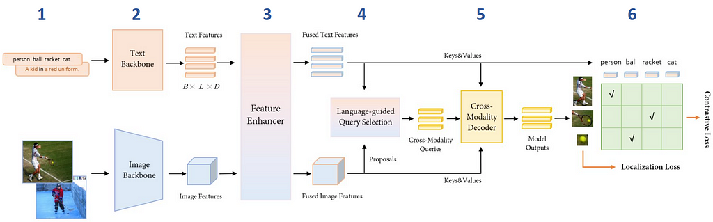
1. The model takes pairs of image and text description as inputs.
2. Image features are extracted with an image backbone such as Swin Transformer, and text features with a text backbone like BERT.
3. To fuse image and text modalities into a single representation, both types of features are fed into the Feature Enhancer module.
4. Next, the ‘Language-guided Query Selection’ module selects the features most relevant to the input text to use as decoder queries.
5. These queries are then fed into a decoder to refine the prediction of object detection boxes that best align with the text information.
6. The model outputs 900 object bounding boxes and their similarity scores to the input words. The boxes with similarity scores above the box_threshold are chosen, and words whose similarities are higher than the text_threshold as predicted labels.

Prompt Engineering

The GroundingDino model encodes text prompts into a learned latent space. Altering the prompts can lead to different text features, which can affect the performance of the detector. To enhance prediction performance, it’s advisable to experiment with multiple prompts, choosing the one that delivers the best results. It’s important to note that while writing this article I had to try several prompts before finding the ideal one, sometimes encountering unexpected results.

Code Implementation

Getting Started

To begin, we’ll clone the GroundingDino repository from GitHub, set up the environment by installing the necessary dependencies, and download the pre-trained model weights.

# Clone:
!git clone https://github.com/IDEA-Research/GroundingDINO.git

# Install
%cd GroundingDINO/
!pip install -r requirements.txt
!pip install -q -e .

# Get weights
!wget -q https://github.com/IDEA-Research/GroundingDINO/releases/download/v0.1.0-alpha/groundingdino_swint_ogc.pth

Inference on an image

We’ll start our exploration of the object detection algorithm by applying it to a single image of tomatoes. Our initial goal is to detect all the tomatoes in the image, so we’ll use the text prompt tomato. If you want to use different category names, you can separate them with a dot .. Note that the colors of the bounding boxes are random and have no particular meaning.

python3 demo/inference_on_a_image.py 
    --config_file 'groundingdino/config/GroundingDINO_SwinT_OGC.py' 
    --checkpoint_path 'groundingdino_swint_ogc.pth' 
    --image_path 'tomatoes_dataset/tomatoes1.jpg'  
    --text_prompt 'tomato' 
    --box_threshold 0.35 
    --text_threshold 0.01 
    --output_dir 'outputs'

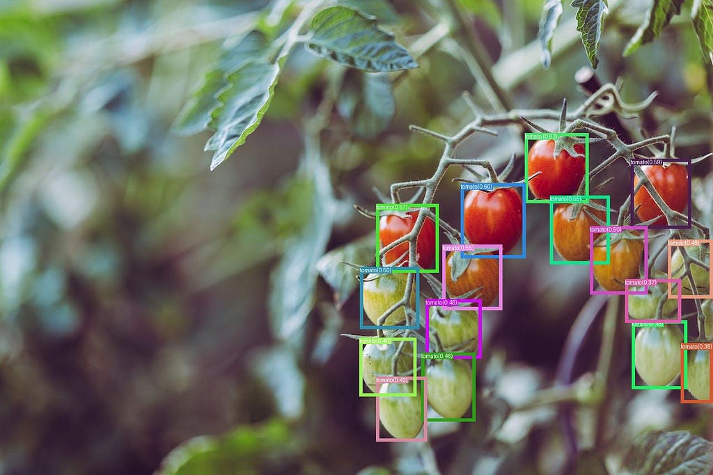
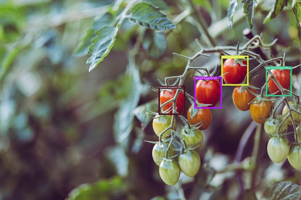
GroundingDino not only detects objects as categories, such as tomato, but also comprehends the input text, a task known as Referring Expression Comprehension (REC). Let’s change the text prompt from tomato to ripened tomato, and obtain the outcome:

python3 demo/inference_on_a_image.py 
    --config_file 'groundingdino/config/GroundingDINO_SwinT_OGC.py' 
    --checkpoint_path 'groundingdino_swint_ogc.pth' 
    --image_path 'tomatoes_dataset/tomatoes1.jpg'  
    --text_prompt 'ripened tomato' 
    --box_threshold 0.35 
    --text_threshold 0.01 
    --output_dir 'outputs'

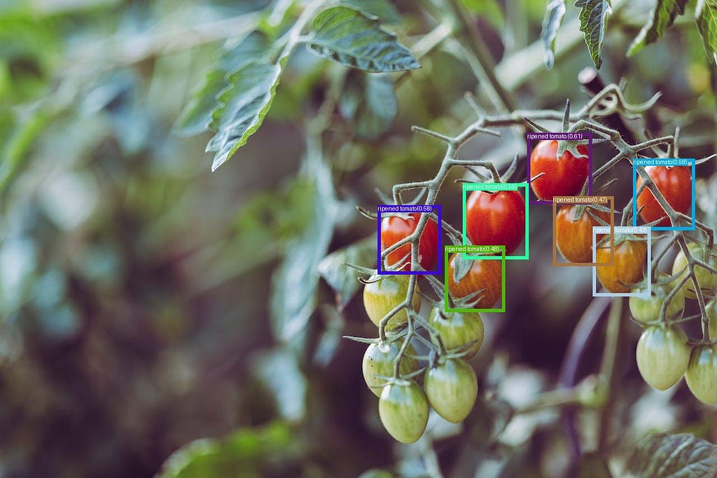
Remarkably, the model can ‘understand’ the text and differentiate between a ‘tomato’ and a ‘ripened tomato’. It even tags partially ripened tomatoes that aren’t fully red. If our task requires tagging only fully ripened red tomatoes, we can adjust the box_threshold from the default 0.35 to 0.5.

python3 demo/inference_on_a_image.py 
    --config_file 'groundingdino/config/GroundingDINO_SwinT_OGC.py' 
    --checkpoint_path 'groundingdino_swint_ogc.pth' 
    --image_path 'tomatoes_dataset/tomatoes1.jpg'  
    --text_prompt 'ripened tomato' 
    --box_threshold 0.5 
    --text_threshold 0.01 
    --output_dir 'outputs'

Generation of tagged dataset

Even though GroundingDino has remarkable capabilities, it’s a large and slow model. If real-time object detection is needed, consider using a faster model like YOLO. Training YOLO and similar models require a lot of tagged data, which can be expensive and time-consuming to produce. However, if your data isn’t unique, you can use GroundingDino to tag it. To learn more about efficient YOLO training, refer to my previous article [4].

The GroundingDino repository includes a script to annotate image datasets in the COCO format, which is suitable for YOLOx, for instance.

from demo.create_coco_dataset import main

main(image_directory= 'tomatoes_dataset',
    text_prompt= 'tomato',
    box_threshold= 0.35,
    text_threshold = 0.01,
    export_dataset = True,
    view_dataset = False,
    export_annotated_images = True,
    weights_path = 'groundingdino_swint_ogc.pth',
    config_path = 'groundingdino/config/GroundingDINO_SwinT_OGC.py',
    subsample = None
)

• export_dataset — If set to True, the COCO format annotations will be saved in a directory named ‘coco_dataset’.
• view_dataset — If set to True, the annotated dataset will be displayed for visualization in the FiftyOne app.
• export_annotated_images — If set to True, the annotated images will be stored in a directory named ‘images_with_bounding_boxes’.
• subsample (int) — If specified, only this number of images from the dataset will be annotated.

Different YOLO algorithms require different annotation formats. If you’re planning to train YOLOv5 or YOLOv8, you’ll need to export your dataset in the YOLOv5 format. Although the export type is hard-coded in the main script, you can easily change it by adjusting the dataset_type argument in create_coco_dataset.main, from fo.types.COCODetectionDataset to fo.types.YOLOv5Dataset(line 72). To keep things organized, we’ll also change the output directory name from ‘coco_dataset’ to ‘yolov5_dataset’. After changing the script, run create_coco_dataset.main again.

  if export_dataset:
      dataset.export(
          'yolov5_dataset',
          dataset_type=fo.types.YOLOv5Dataset
      )

Concluding remarks

GroundingDino offers a significant leap in object detection annotations by using text prompts. In this tutorial, we have explored how to use the model for automated labeling of an image or a whole dataset. It’s crucial, however, to manually review and verify these annotations before they are utilized in training subsequent models.

_________________________________________________________________

A user-friendly Jupyter notebook containing the complete code is included for your convenience:

Thank you for reading!

Want to learn more?

• Explore additional articles I’ve written
• Subscribe to get notified when I publish articles
• Follow me on Linkedin

References

[1] Grounding DINO: Marrying DINO with Grounded Pre-Training for Open-Set Object Detection, 2023.

[2] Dino: Detr with improved denoising anchor boxes for end-to-end object detection, 2022.

[3] An Open and Comprehensive Pipeline for Unified Object Grounding and Detection, 2023.

[4] The practical guide for Object Detection with YOLOv5 algorithm, by Dr. Lihi Gur Arie.

---

Automatic Labeling of Object Detection Datasets Using GroundingDino was originally published in Towards Data Science on Medium, where people are continuing the conversation by highlighting and responding to this story.

How Neural Networks are strong tools for solving differential equations without the use of training data

Differential equations are one of the protagonists in physical sciences, with vast applications in engineering, biology, economy, and even social sciences. Roughly speaking, they tell us how a quantity varies in time (or some other parameter, but usually we are interested in time variations). We can understand how a population, or a stock price, or even how the opinion of some society towards certain themes changes over time.

Typically, the methods used to solve DEs are not analytical (i.e. there is no “closed formula” for the solution) and we have to resource to numerical methods. However, numerical methods can be expensive from a computational standpoint, and worse than that: the accumulated error can be significantly large.

This article will showcase how a Neural Network can be a valuable ally to solve a differential equation, and how we can borrow concepts from Physics-Informed Neural Networks to tackle the question: can we use a machine learning approach to solve a DE?

A pinch of Physics-Informed Neural Networks

In this section, I will talk about Physics-Informed Neural Networks very briefly. I suppose you know the “neural network” part, but what makes them be informed by physics? Well, they are not exactly informed by physics, but rather by a (differential) equation.

Usually, neural networks are trained to find patterns and figure out what’s going on with a set of training data. However, when you train a neural network to obey the behavior of your training data and hopefully fit unseen data, your model is highly dependent on the data itself, and not on the underlying nature of your system. It sounds almost like a philosophical matter, but it is more practical than that: if your data comes from measurements of ocean currents, these currents have to obey the physics equations that describe ocean currents. Notice, however, that your neural network is completely agnostic about these equations and is only trying to fit data points.

This is where physics informed comes into play. If, besides learning how to fit your data, your model also learns how to fit the equations that govern that system, the predictions of your neural network will be much more precise and will generalize much better, just citing some advantages of physics-informed models.

Notice that the governing equations of your system don’t have to involve physics at all, the “physics-informed” thing is just nomenclature (and the technique is most used by physicists anyway). If your system is the traffic in a city and you happen to have a good mathematical model that you want your neural network’s predictions to obey, then physics-informed neural networks are a good fit for you.

How do we inform these models?

Hopefully, I’ve convinced you that it is worth the trouble to make the model aware of the underlying equations that govern our system. However, how can we do this? There are several approaches to this, but the main one is to adapt the loss function to have a term that accounts for the governing equations, aside from the usual data-related part. That is, the loss function L will be composed of the sum

Here, the data loss is the usual one: a mean squared difference, or some other suited form of loss function; but the equation part is the charming one. Imagine that your system is governed by the following differential equation:

How can we fit this into the loss function? Well, since our task when training a neural network is to minimize the loss function, what we want is to minimize the following expression:

So our equation-related loss function turns out to be

that is, it is the mean difference squared of our DE. If we manage to minimize this (a.k.a. make this term as close to zero as possible) we automatically satisfy the system’s governing equation. Pretty clever, right?

Now, the extra term L_IC in the loss function needs to be addressed: it accounts for the initial conditions of the system. If a system’s initial conditions are not provided, there are infinitely many solutions for a differential equation. For instance, a ball thrown from the ground level has its trajectory governed by the same differential equation as a ball thrown from the 10th floor; however, we know for sure that the paths made by these balls will not be the same. What changes here are the initial conditions of the system. How does our model know which initial conditions we are talking about? It is natural at this point that we enforce it using a loss function term! For our DE, let’s impose that when t = 0, y = 1. Hence, we want to minimize an initial condition loss function that reads:

If we minimize this term, then we automatically satisfy the initial conditions of our system. Now, what is left to be understood is how to use this to solve a differential equation.

Solving a differential equation

If a neural network can be trained either with the data-related term of the loss function (this is what is usually done in classical architectures), and can also be trained with both the data and the equation-related term (this is physics-informed neural networks I just mentioned), it must be true that it can be trained to minimize only the equation-related term. This is exactly what we are going to do! The only loss function used here will be the L_equation. Hopefully, this diagram below illustrates what I’ve just said: today we are aiming for the right-bottom type of model, our DE solver NN.

Code implementation

To showcase the theoretical learnings we’ve just got, I will implement the proposed solution in Python code, using the PyTorch library for machine learning.

The first thing to do is to create a neural network architecture:

import torch
import torch.nn as nn

class NeuralNet(nn.Module):
    def __init__(self, hidden_size, output_size=1,input_size=1):
        super(NeuralNet, self).__init__()
        self.l1 = nn.Linear(input_size, hidden_size)
        self.relu1 = nn.LeakyReLU()
        self.l2 = nn.Linear(hidden_size, hidden_size)
        self.relu2 = nn.LeakyReLU()
        self.l3 = nn.Linear(hidden_size, hidden_size)
        self.relu3 = nn.LeakyReLU()
        self.l4 = nn.Linear(hidden_size, output_size)

    def forward(self, x):
        out = self.l1(x)
        out = self.relu1(out)
        out = self.l2(out)
        out = self.relu2(out)
        out = self.l3(out)
        out = self.relu3(out)
        out = self.l4(out)
        return out

This one is just a simple MLP with LeakyReLU activation functions. Then, I will define the loss functions to calculate them later during the training loop:

# Create the criterion that will be used for the DE part of the loss
criterion = nn.MSELoss()

# Define the loss function for the initial condition
def initial_condition_loss(y, target_value):
    return nn.MSELoss()(y, target_value)

Now, we shall create a time array that will be used as train data, and instantiate the model, and also choose an optimization algorithm:

# Time vector that will be used as input of our NN
t_numpy = np.arange(0, 5+0.01, 0.01, dtype=np.float32)
t = torch.from_numpy(t_numpy).reshape(len(t_numpy), 1)
t.requires_grad_(True)

# Constant for the model
k = 1

# Instantiate one model with 50 neurons on the hidden layers
model = NeuralNet(hidden_size=50)

# Loss and optimizer
learning_rate = 8e-3
optimizer = torch.optim.SGD(model.parameters(), lr=learning_rate)

# Number of epochs
num_epochs = int(1e4)

Finally, let’s start our training loop:

for epoch in range(num_epochs):

    # Randomly perturbing the training points to have a wider range of times
    epsilon = torch.normal(0,0.1, size=(len(t),1)).float()
    t_train = t + epsilon

    # Forward pass
    y_pred = model(t_train)

    # Calculate the derivative of the forward pass w.r.t. the input (t)
    dy_dt = torch.autograd.grad(y_pred, 
                                t_train, 
                                grad_outputs=torch.ones_like(y_pred), 
                                create_graph=True)[0]

    # Define the differential equation and calculate the loss
    loss_DE = criterion(dy_dt + k*y_pred, torch.zeros_like(dy_dt))

    # Define the initial condition loss
    loss_IC = initial_condition_loss(model(torch.tensor([[0.0]])), 
                                     torch.tensor([[1.0]]))

    loss = loss_DE + loss_IC

    # Backward pass and weight update
    optimizer.zero_grad()
    loss.backward()
    optimizer.step()

Notice the use of torch.autograd.grad function to automatically differentiate the output y_pred with respect to the input t to compute the loss function.

Results

After training, we can see that the loss function rapidly converges. Fig. 2 shows the loss function plotted against the epoch number, with an inset showing the region where the loss function has its fastest drop.

You probably have noticed that this neural network is not a common one. It has no train data (our train data was a hand-crafted vector of timestamps, which is simply the time domain that we wanted to investigate), so all information it gets from the system comes in the form of a loss function. Its only purpose is to solve a differential equation within the time domain it was crafted to solve. Hence, to test it, it’s only fair that we use the time domain it was trained on. Fig. 3 shows a comparison between the NN prediction and the theoretical answer (that is, the analytical solution).

We can see a pretty good agreement between the two, which is very good for the neural network.

One caveat of this approach is that it does not generalize well for future times. Fig. 4 shows what happens if we slide our time data points five steps ahead, and the result is simply mayhem.

Hence, the lesson here is that this approach is made to be a numerical solver for differential equations within a time domain, and it should not be used as a regular neural network to make predictions with unseen out-of-train-domain data and expect it to generalize well.

Conclusion

After all, one remaining question is:

Why bother to train a neural network that does not generalize well to unseen data, and on top of that is obviously worse than the analytical solution, since it has an intrinsic statistical error?

First, the example provided here was an example of a differential equation whose analytical solution is known. For unknown solutions, numerical methods must be used nevertheless. With that being said, numerical methods for differential equation solving usually accumulate error. That means if you try to solve the equation for many time steps, the solution will lose its accuracy along the way. The neural network solver, on the other hand, learns how to solve the DE for all data points at each of its training epochs.

Another reason is that neural networks are good interpolators, so if you want to know the value of the function in unseen data (but this “unseen data” has to lie within the time interval you trained) the neural network will promptly give you a value that classic numeric methods will not be able to promptly give.

References

[1] Marios Mattheakis et al., Hamiltonian neural networks for solving equations of motion, arXiv preprint arXiv:2001.11107v5, 2022.

[2] Mario Dagrada, Introduction to Physics-informed Neural Networks, 2022.

---

Solving Differential Equations With Neural Networks was originally published in Towards Data Science on Medium, where people are continuing the conversation by highlighting and responding to this story.

Exploring the Vulnerabilities in Detecting AI-Generated Media

Why do we Need Watermarks?

Watermarks are all over the internet — and for obvious reasons. How else could you protect your art or photography from ending up in someone’s PowerPoint presentation without crediting the creator? The simplest way of addressing this problem is to create visible watermarks like the one below.

The primary downside of this method is that it can compromise the art itself. No one would purchase and use the cat image like this. Therefore, while mitigating unauthorized copies, perceptible watermarks can also discourage the target audience from using the art.

In the music domain, perceptible watermarks are also common in free Hip-Hop beats. Beat producers often insert a voice sample with their brand name right before the first verse starts. This can serve either as a safeguard against illegal downloads or as a marketing tool when the beat is free-to-use.

For stock photos and Hip-Hop beats alike, a common practice is to place watermarks on the online previews and send the original product to clients after payment. However, this is also prone to misuse. As soon as the watermark-free product is purchased, it can be copied and reuploaded to the internet.

The Case for Imperceptible Watermarks

Protection of Intellectual Property

Imperceptible watermarks come with a distinct advantage: You can prove ownership over any digital copy of your product without negatively affecting product quality. It’s like a piece of paper with invisible ink on it. The paper is fully functional, but it carries a secret message that can be revealed at any time.

With this technology, creators can encode any kind of message within their works. More importantly, as they have access to the decoder, they can always assert ownership over any digital copy of their original work. Another emerging opportunity for rights-holders is to use web crawlers to search the web and report any detected misuse.

Detection of AI-Generated Content

Another valuable application for imperceptible watermarks is for detecting AI-generated content. The advent of ChatGPT and similar AI tools has raised concerns about the potential overflow of dangerous AI-generated content on the internet. Tech companies like Meta or Google are bringing forward imperceptible watermarking systems as technological breakthroughs to mitigate this problem. Their tools can add watermarks to images or music without any noticeable change in quality.

In principle, this is a noteworthy development. With imperceptible watermarks, only the owner of the technology can decode and detect the presence of such watermarks. Using our example from above, Meta & Google own both the invisible ink and the means to reveal it. This allows them to accurately detect and filter content generated with their own tools on their platforms (e.g. Instagram, YouTube). Through collaborations, even independent platforms like X (former Twitter) could use this tech to limit AI-generated misinformation or other harmful content.

How can AI Remove Imperceptible Watermarks?

Although imperceptible watermarks sound promising and are being promoted by big tech companies, they are far from perfect. In fact, many of these watermarks can be reliably removed using smart AI algorithms. But how can AI remove something that is imperceptible?

Removing Perceptible Watermarks

Let’s start by understanding how perceptible watermarks can be removed with AI. Let me propose a simple approach: Start by collecting hundreds of thousands of images from the web. Then, automatically add artificial watermarks to these images. Make sure they resemble real watermarks and cover a wide variety of fonts, sizes, and styles. Then, train an AI to remove watermarks by repeatedly showing it pairs of the same image — once with and once without the watermark.

While there are certainly more sophisticated approaches, this illustrates the ease with which watermarks can be removed if the AI is trained to recognize their appearance or sound. There are numerous tools online that allow me to easily remove the watermark from my cat image above:

Removing Imperceptible Watermarks

To employ this simple approach from above, you need to provide the AI with the “before and after” examples. However, if the watermarks are imperceptible, how can find these examples? Even worse, we can’t even tell if a watermark is present or not just by looking at an image or listening to a song.

To solve this problem, researchers had to get creative. Zhao et al., 2023 came up with a two-stage procedure.

1. Destroy the watermark by adding random noise to the image
2. Reconstruct the real image by using a denoising algorithm

This is brilliant, because it challenges the intuition that, in order to remove a watermark, you must be able to detect it. This approach can’t locate the watermark. However, if the only goal is to remove the watermark, simply destroying it by adding enough white noise to the image is quick and effective.

Of course, after adding noise, you might have broken the watermark, but you end up with a noisy picture. The most fascinating part is how the authors then reconstructed the original image from the noise. For that, they used AI diffusion models, such as the ones used in DALL-E 3 or Midjourney. These models generate images by iteratively turning random noise into realistic pictures.

As a side effect, diffusion models are also incredibly effective denoising systems, both for images and for audio. By leveraging this technology, anyone can remove imperceptible watermarks using this exact two-step procedure.

Does this Mean Imperceptible Watermarks are Useless?

Yes and no. On the one hand, it seems likely that any imperceptible watermarking system invented so far can be broken by bad actors through one method or the other. When I posted about this problem on Linkedin for the first time, one person commented: “It’s the adblocker blocker blocker game all over again”, and I couldn’t agree more.

The obvious defence against the attack approach proposed by Zhao et al. (2023) is to develop an invisible watermarking system that is robust to it. For instance, we could train our watermarking system in a way that current SOTA diffusion models cannot reconstruct the image well after removing the watermark with random noise. Or we could try to build a watermark that is robust to random noise attacks. In either case, new vulnerabilities would quickly be found and exploited.

So are imperceptible watermarks simply useless? In a recent article, Sharon Goldman argues that while watermarks might not stop bad actors, they could still be beneficial for good actors. They are a bit like metadata, but encoded directly into the object of interest. Unlike MP3 metadata, which may be lost when the audio is converted to a different format, imperceptible watermarks would always be traceable, as they are embedded directly in the music itself.

However, if I am honest with myself, I was hopeful that imperceptible watermarks could be a viable solution to flagging and detecting AI-generated content. Apparently, I was wrong. These watermarks will not prevent bad actors from flooding the internet with harmful AI-generated content, by and large.

How Else Can We Prove Ownership in the AI Era?

Development of Countermeasures

As highlighted above, developing countermeasures to known attack algorithms is always an option. In many cases, however, it is easier for the attackers to iterate on their attack algorithms than for the defenders to develop safeguards. Still, we can’t neglect the possibility that we might discover a new approach to watermarking that isn’t as easily breakable. It is therefore definitely worth investing time and resources into further research on this topic.

Legal Consequences Against Watermark Attackers

While generating images with AI and uploading them to a social media platform is generally not considered illegal, purposefully removing watermarks from AI-generated images could very well be. Having no legal expertise myself, I can only argue that it would make sense to threaten legal consequences against such malicious actions.

Of course, the normal users resharing images they found online should be excluded from this. However, purposefully removing watermarks to spread misinformation is clearly immoral. And even if legal pressure will not eradicate misuse (it never has), it can be one mitigating factor.

Rethinking Proofs of Ownership

Many approaches exist around how blockchain technology and/or smart contracts could help prove ownership in the digital age. A blockchain, in simple terms, is a information storage that tracks interactions between members of a network. Each transaction can be uniquely identified and can’t be manipulated at any later point in time. Adding smart contracts to this network allows us to connect transactions to binding responsibilities that are automatically fulfilled once the transaction is done.

In less abstract terms, blockchains and smart contracts could be used in the future to automate ownership checks or royalty payments for intellectual property in any shape or form. So far, no such system has found widespread adoption. Still, we might be only a few technical breakthroughs away from these technologies becoming invaluable assets in our economies.

Conclusion

Digital watermarks have been used since the the early days of the internet to prevent misuse of intellectual property such as images or music. Recently, it has been discussed as a method for flagging and detecting AI generated content. However, it turns out that AI is not only great at generating fake images. It is just as good at removing any kind of watermark on these images, rendering most detection systems useless.

It is clear that we can’t let this discourage us in searching for alternative ways of proving ownership in the age of AI. By developing concrete technical and legal countermeasures and, at the same time, exploring how blockchains and/or smart contracts could be leveraged in the future, we might just figure out how to solve this important problem.

References

Zhao et al., 2023. Invisible Image Watermarks Are Provably Removable Using Generative AI. https://arxiv.org/pdf/2306.01953.pdf

About Me

I’m a musicologist and a data scientist, sharing my thoughts on current topics in AI & music. Here is some of my previous work related to this article:

• 3 Music AI Breakthroughs to Expect in 2024: https://towardsdatascience.com/3-music-ai-breakthroughs-to-expect-in-2024-2d945ae6b5fd
• How Meta’s AI Generates Music Based on a Reference Melody: https://medium.com/towards-data-science/how-metas-ai-generates-music-based-on-a-reference-melody-de34acd783
• AI Music Source Separation: How it Works and Why it is so Hard: https://medium.com/towards-data-science/ai-music-source-separation-how-it-works-and-why-it-is-so-hard-187852e54752

Find me on Medium and Linkedin!

---

How AI Can Remove Imperceptible Watermarks was originally published in Towards Data Science on Medium, where people are continuing the conversation by highlighting and responding to this story.

Navigating Slowly Changing Dimensions (SCD) and Data Restatement: A Comprehensive Guide

Strategies for efficiently managing dimension changes and data restatement in enterprise data warehousing

Imagine this, you are a data engineer working for a large retail company that utilizes the incremental load technique in data warehousing. This technique involves selectively updating or loading only the new or modified data since the last update. What could occur when the product R&D department decides to change the name or description of a current product? How would such updates impact your existing data pipeline and data warehouse? How do you plan to address challenges like these? This article provides a comprehensive guide with solutions, utilizing Slowly Changing Dimensions (SCD), to tackle potential issues during data restatement.

What are Slowly Changing Dimensions (SCD)?

Slowly changing dimensions refer to infrequent changes in dimension values, which occur sporadically and are not tied to a daily or regular time-based schedule, as dimensions typically change less frequently than transaction entries in a system. For example, a jewelry company that has its customers placing a new order on their website will become a new row in the order fact table. On the other hand, the jewelry company rarely changes their product name and their product description but that doesn’t mean it will never happen in the future.

Managing changes in these dimensions requires employing Slowly Changing Dimension (SCD) management techniques, which are categorized into defined SCD types, ranging from Type 0 through Type 6, including some combination or hybrid types. We can employ one of the following methods:

SCD Type 0: Ignore

Changes to dimension values are completely disregarded, and the values of dimensions remain unchanged from the time they were initially created in the data warehouse.

SCD Type 1: Overwrite/ Replace

This approach is applicable when the previous value of the dimension attribute is no longer relevant or important. However, historical tracking of changes is not necessary.

SCD Type 2: Create a New Dimension Row

This approach is recommended as the primary technique for addressing changing dimension values, involving the creation of a second row for the dimension with a start date, end date, and potentially a “current/expired” flag. It is suitable for our scenarios like product description or address changes, ensuring a clear partitioning of history. The new dimension row is linked to newly inserted fact rows, with each dimension record linked to a subset of fact rows based on insertion times — those before the change linked to the old dimension row, and those after linked to the new dimension row.

SCD Type 3: Create a “PREV” Column

This method is suitable when both the old and new values are relevant, and users may want to conduct historical analysis using either value. However, it is not practical to apply this technique to all dimension attributes, as it would involve providing two columns for each attribute in dimension tables or more if multiple “PREV” values need preservation. It should be selectively used where appropriate.

SCD Type 4: Rapidly Changing Large Dimensions

What if in a scenario you need to capture every change to every dimension attribute for a very large dimension of retail, say a million plus customers of your huge jewelry company? Using type 2 above will very quickly explode the number of rows in the customer dimension table to tens or even hundreds of millions of rows and using type 3 is not viable.

A more effective solution for rapidly changing and large volume dimension tables is to categorize attributes (e.g., customer age category, gender, purchasing power, birthday, etc.) and separate them into a secondary dimension, like a customer profile dimension. This table, acting as a “full coverage” dimension table all potential values for every category of dimension attributes preloaded into the table, which can better manage the granularity of changes while avoiding excessive row expansion in the main customer dimension.

For example, if we have 8 age categories, 3 different genders, 6 purchasing power categories, and 366 possible birthdays. Our “full coverage” dimension table for customer profiles that contains all the above combinations will be 8 x 3 x 6 x 366 combinations or 52704 rows.

We’ll need to generate surrogate_key for this dimension table and establish a connection to a new foreign key in the fact table. When a modification occurs in one of these dimension categories, there’s no necessity to add another row to the customer dimension. Instead, we generate a new fact row and associate it with both the customer dimension and the new customer profile dimension.

SCD Type 5: An Extension to Type 4

To enhance the Type 4 approach mentioned earlier, we can establish a connection between the customer dimension and the customer profile dimension. This linkage enables the tracking of the “current” customer profile for a specific customer. The key facilitates the connection of the customer with the latest customer profile, which allows seamless traversal from the customer dimension to the most recent customer profile dimension without the need to link through the fact table.

SCD Type 6: A Hybrid Technique

With this approach, you integrate both Type 2 (new row) and Type 3 (“PREV” column). This blended approach offers the advantages of both methodologies. You can retrieve facts using the “ PREV “ column, which provides historical values and presents facts associated with the product category at that specific time. Simultaneously, querying by the “new” column provides all facts for both the current and all preceding values of the product category.

Bonus and Conclusion

Normally, data extraction comes in STAR schema, which includes one fact table and multiple dimension tables in an enterprise. While the dimension tables store all the descriptive data and primary keys, the fact table contains numeric and additive data that references the primary keys of each dimension around it.

However, if your marketing sales data extract is provided as a single denormalized table without distinct dimension tables and lacks the primary key for its descriptive data, future updates to product names may pose challenges. Handling such scenarios in your existing pipeline can be more complicated.

The absence of primary keys in the descriptive data can lead to issues during data restatement, especially when you are dealing with large datasets. For instance, if a product name is updated in the restatement extract without a unique product_key, the incremental load pipeline may treat it as a new product, impacting the historical data in your consumption layer. To address this, creating surrogate_key for the product dimension and a mapping table to link original and restated product names is necessary for maintaining data integrity.

In conclusion, every aspect of data warehouse design should be carefully considered, taking into account potential edge cases.

---

Navigating Slowly Changing Dimensions (SCD) and Data Reinstatement: A Comprehensive Guide was originally published in Towards Data Science on Medium, where people are continuing the conversation by highlighting and responding to this story.

Launched in 2021, Amazon SageMaker Canvas is a visual, point-and-click service for building and deploying machine learning (ML) models without the need to write any code. Ready-to-use Foundation Models (FMs) available in SageMaker Canvas enable customers to use generative AI for tasks such as content generation and summarization. We are thrilled to announce the latest […]