

Originally appeared here:
MultiChoice Question Answering In HuggingFace
Go Here to Read this Fast! MultiChoice Question Answering In HuggingFace

Originally appeared here:
Accenture creates a regulatory document authoring solution using AWS generative AI services

For a data engineer building analytics from transactional systems such as ERP (enterprise resource planning) and CRM (customer relationship management), the main challenge lies in navigating the gap between raw operational data and domain knowledge. ERP and CRM systems are designed and built to fulfil a broad range of business processes and functions. This generalisation makes their data models complex and cryptic and require domain expertise.
Even harder to manage, a common setup within large organisations is to have several instances of these systems with some underlaying processes in charge of transmitting data among them, which could lead to duplications, inconsistencies, and opacity.
The disconnection between the operational teams immersed in the day-to-day functions and those extracting business value from data generated in the operational processes still remains a significant friction point.
Imagine being a data engineer/analyst tasked with identifying the top-selling products within your company. Your first step might be to locate the orders. Then you begin researching database objects and find a couple of views, but there are some inconsistencies between them so you do not know which one to use. Additionally, it is really hard to identify the owners, one of them has even recently left the company. As you do not want to start your development with uncertainty, you decide to go for the operational raw data directly. Does it sound familiar?
I used to connect to views in transactional databases or APIs offered by operational systems to request the raw data.
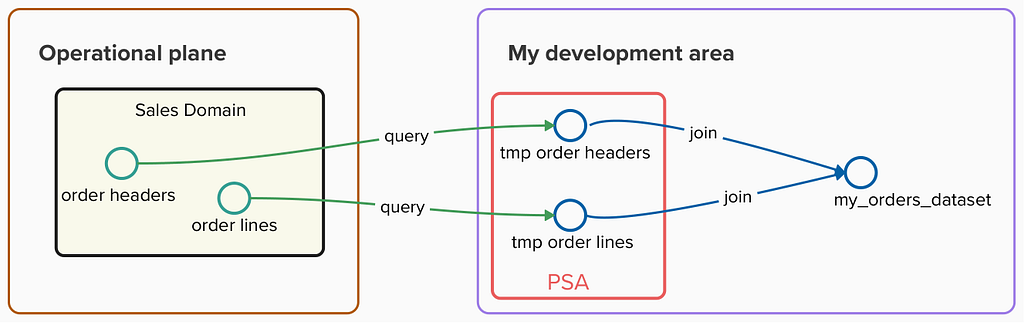
To prevent my extractions from impacting performance on the operational side, I queried this data regularly and stored it in a persistent staging area (PSA) within my data warehouse. This allowed me to execute complex queries and data pipelines using these snapshots without consuming any resource from operational systems, but could result in unnecessary duplication of data in case I was not aware of other teams doing the same extraction.
Once the raw operational data was available, then I needed to deal with the next challenge: deciphering all the cryptic objects and properties and dealing with the labyrinth of dozens of relationships between them (i.e. General Material Data in SAP documented https://leanx.eu/en/sap/table/mara.html)
Even though standard objects within ERP or CRM systems are well documented, I needed to deal with numerous custom objects and properties that require domain expertise as these objects cannot be found in the standard data models. Most of the time I found myself throwing ‘trial-and-error’ queries in an attempt to align keys across operational objects, interpreting the meaning of the properties according to their values and checking with operational UI screenshots my assumptions.
A Data Mesh implementation improved my experience in these aspects:
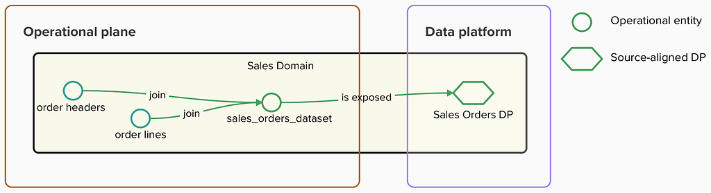
According to the Data Mesh taxonomy, data products built on top of operational sources are named Source-aligned Data Products:
Source domain datasets represent closely the raw data at the point of creation, and are not fitted or modelled for a particular consumer — Zhamak Dehghani
Source-aligned data products aim to represent operational sources within a shared data platform in a one-to-one relationship with operational entities and they should not hold any business logic that could alter any of their properties.
In a Data Mesh implementation, these data products should
strictly be owned by the business domain that generates the raw data. The owner is responsible for the quality, reliability, and accessibility of their data and data is treated as a product that can be used by the same team and other data teams in other parts of the organisation.
This ownership ensures domain knowledge is close to the exposed data. This is critical to enabling the fast development of analytical data products, as any clarification needed by other data teams can be handled quickly and effectively.
Following this approach, the Sales domain is responsible for publishing a ‘sales_orders’ data product and making it available in a shared data catalog.
The data pipeline in charge of maintaining the data product could be defined like this:
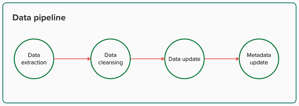
Data extraction
The first step to building source-aligned data products is to extract the data we want to expose from operational sources. There are a bunch of Data Integration tools that offer a UI to simplify the ingestion. Data teams can create a job there to extract raw data from operational sources using JDBC connections or APIs. To avoid wasting computational work, and whenever possible, only the updated raw data since the last extraction should be incrementally added to the data product.
Data cleansing
Now that we have obtained the desired data, the next step involves some curation, so consumers do not need to deal with existing inconsistencies in the real sources. Although any business logic should not not be implemented when building source-aligned data products, basic cleansing and standardisation is allowed.
-- Example of property standardisation in a sql query used to extract data
case
  when lower(SalesDocumentCategory) = 'invoice' then 'Invoice'
  when lower(SalesDocumentCategory) = 'invoicing' then 'Invoice'
  else SalesDocumentCategory
end as SALES_DOCUMENT_CATEGORY
Data update
Once extracted operational data is prepared for consumption, the data product’s internal dataset is incrementally updated with the latest snapshot.
One of the requirements for a data product is to be interoperable. This means that we need to expose global identifiers so our data product might be universally used in other domains.
Metadata update
Data products need to be understandable. Producers need to incorporate meaningful metadata for the entities and properties contained. This metadata should cover these aspects for each property:
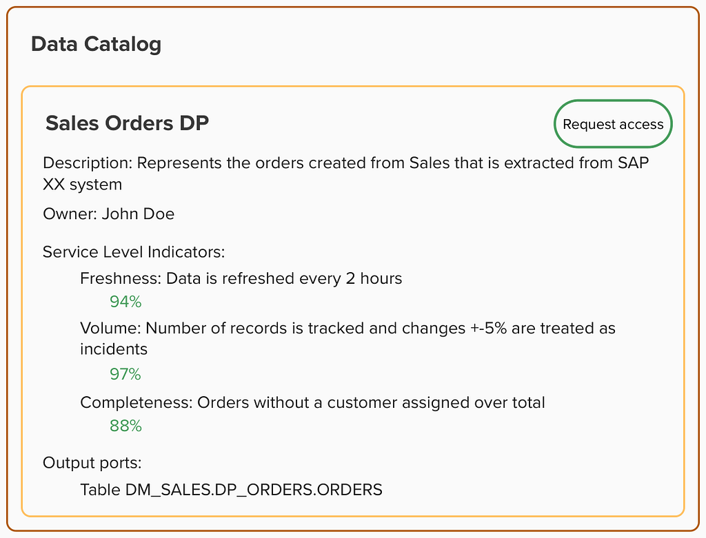
Data products also need to be discoverable. Producers need to publish them in a shared data catalog and indicate how the data is to be consumed by defining output port assets that serve as interfaces to which the data is exposed.
And data products must be observable. Producers need to deploy a set of monitors that can be shown within the catalog. When a potential consumer discovers a data product in the catalog, they can quickly understand the health of the data contained.
Now, again, imagine being a data engineer tasked with identifying the top-selling products within your company. But this time, imagine that you have access to a data catalog that offers data products that represent the truth of each domain shaping the business. You simply input ‘orders’ into the data product catalog and find the entry published by the Sales data team. And, at a glance, you can assess the quality and freshness of the data and read a detailed description of its contents.
This upgraded experience eliminates the uncertainties of traditional discovery, allowing you to start working with the data right away. But what’s more, you know who is accountable for the data in case further information is needed. And whenever there is an issue with the Sales orders data product, you will receive a notification so that you can take actions in advance.
We have identified several benefits of enabling operational data through source-aligned data products, especially when they are owned by data producers:
Based on my own experience, this approach works exceptionally well in scenarios where large organisations struggle with data inconsistencies across different domains and friction when building their own analytics on top of operational data. Data Mesh encourages each domain to build the ‘source of truth’ for the core entities they generate and make them available in a shared catalog allowing other teams to access them and create consistent metrics across the whole organisation. This enables analytical data teams to accelerate their work in generating analytics that drive real business value.
How to Move Beyond a Monolithic Data Lake to a Distributed Data Mesh
https://www.oreilly.com/library/view/data-mesh/9781492092384/
Thanks to my Thoughtworks colleagues Arne (twice!), Pablo, Ayush and Samvardhan for taking the time to review the early versions of this article
A Data Mesh Implementation: Expediting Value Extraction from ERP/CRM Systems was originally published in Towards Data Science on Medium, where people are continuing the conversation by highlighting and responding to this story.
Originally appeared here:
A Data Mesh Implementation: Expediting Value Extraction from ERP/CRM Systems

Creating an animation from geostationary satellite images to dynamically monitor storms in real-time using Python and Google Colab
Originally appeared here:
Watching Storms from Space: A Python Script for Creating an Amazing View
Go Here to Read this Fast! Watching Storms from Space: A Python Script for Creating an Amazing View

Super Bowl Sunday has historically captivated the American audience by catering to diverse interests. Football fanatics are enthralled by…
Originally appeared here:
Optimizing Super Bowl Squares with Linear Programming
Go Here to Read this Fast! Optimizing Super Bowl Squares with Linear Programming

Objects and their relationships are ubiquitous in the world around us, and relationships can be as important to understanding an object as its own attributes viewed in isolation — take for example transportation networks, production networks, knowledge graphs, or social networks. Discrete mathematics and computer science have a long history of formalizing such networks as graphs, consisting of nodes connected by edges in various irregular ways. Yet most machine learning (ML) algorithms allow only for regular and uniform relations between input objects, such as a grid of pixels, a sequence of words, or no relation at all.
Graph neural networks, or GNNs for short, have emerged as a powerful technique to leverage both the graph’s connectivity (as in the older algorithms DeepWalk and Node2Vec) and the input features on the various nodes and edges. GNNs can make predictions for graphs as a whole (Does this molecule react in a certain way?), for individual nodes (What’s the topic of this document, given its citations?) or for potential edges (Is this product likely to be purchased together with that product?). Apart from making predictions about graphs, GNNs are a powerful tool used to bridge the chasm to more typical neural network use cases. They encode a graph’s discrete, relational information in a continuous way so that it can be included naturally in another deep learning system.
We are excited to announce the release of TensorFlow GNN 1.0 (TF-GNN), a production-tested library for building GNNs at large scales. It supports both modeling and training in TensorFlow as well as the extraction of input graphs from huge data stores. TF-GNN is built from the ground up for heterogeneous graphs, where types of objects and relations are represented by distinct sets of nodes and edges. Real-world objects and their relations occur in distinct types, and TF-GNN’s heterogeneous focus makes it natural to represent them.
Inside TensorFlow, such graphs are represented by objects of type tfgnn.GraphTensor. This is a composite tensor type (a collection of tensors in one Python class) accepted as a first-class citizen in tf.data.Dataset, tf.function, etc. It stores both the graph structure and its features attached to nodes, edges and the graph as a whole. Trainable transformations of GraphTensors can be defined as Layers objects in the high-level Keras API, or directly using the tfgnn.GraphTensor primitive.
For illustration, let’s look at one typical application of TF-GNN: predicting a property of a certain type of node in a graph defined by cross-referencing tables of a huge database. For example, a citation database of Computer Science (CS) arXiv papers with one-to-many cites and many-to-one cited relationships where we would like to predict the subject area of each paper.
Like most neural networks, a GNN is trained on a dataset of many labeled examples (~millions), but each training step consists only of a much smaller batch of training examples (say, hundreds). To scale to millions, the GNN gets trained on a stream of reasonably small subgraphs from the underlying graph. Each subgraph contains enough of the original data to compute the GNN result for the labeled node at its center and train the model. This process — typically referred to as subgraph sampling — is extremely consequential for GNN training. Most existing tooling accomplishes sampling in a batch way, producing static subgraphs for training. TF-GNN provides tooling to improve on this by sampling dynamically and interactively.
 |
| Pictured, the process of subgraph sampling where small, tractable subgraphs are sampled from a larger graph to create input examples for GNN training. |
TF-GNN 1.0 debuts a flexible Python API to configure dynamic or batch subgraph sampling at all relevant scales: interactively in a Colab notebook (like this one), for efficient sampling of a small dataset stored in the main memory of a single training host, or distributed by Apache Beam for huge datasets stored on a network filesystem (up to hundreds of millions of nodes and billions of edges). For details, please refer to our user guides for in-memory and beam-based sampling, respectively.
On those same sampled subgraphs, the GNN’s task is to compute a hidden (or latent) state at the root node; the hidden state aggregates and encodes the relevant information of the root node’s neighborhood. One classical approach is message-passing neural networks. In each round of message passing, nodes receive messages from their neighbors along incoming edges and update their own hidden state from them. After n rounds, the hidden state of the root node reflects the aggregate information from all nodes within n edges (pictured below for n = 2). The messages and the new hidden states are computed by hidden layers of the neural network. In a heterogeneous graph, it often makes sense to use separately trained hidden layers for the different types of nodes and edges
 |
| Pictured, a simple message-passing neural network where, at each step, the node state is propagated from outer to inner nodes where it is pooled to compute new node states. Once the root node is reached, a final prediction can be made. |
The training setup is completed by placing an output layer on top of the GNN’s hidden state for the labeled nodes, computing the loss (to measure the prediction error), and updating model weights by backpropagation, as usual in any neural network training.
Beyond supervised training (i.e., minimizing a loss defined by labels), GNNs can also be trained in an unsupervised way (i.e., without labels). This lets us compute a continuous representation (or embedding) of the discrete graph structure of nodes and their features. These representations are then typically utilized in other ML systems. In this way, the discrete, relational information encoded by a graph can be included in more typical neural network use cases. TF-GNN supports a fine-grained specification of unsupervised objectives for heterogeneous graphs.
The TF-GNN library supports building and training GNNs at various levels of abstraction.
At the highest level, users can take any of the predefined models bundled with the library that are expressed in Keras layers. Besides a small collection of models from the research literature, TF-GNN comes with a highly configurable model template that provides a curated selection of modeling choices that we have found to provide strong baselines on many of our in-house problems. The templates implement GNN layers; users need only to initialize the Keras layers.
 |
At the lowest level, users can write a GNN model from scratch in terms of primitives for passing data around the graph, such as broadcasting data from a node to all its outgoing edges or pooling data into a node from all its incoming edges (e.g., computing the sum of incoming messages). TF-GNN’s graph data model treats nodes, edges and whole input graphs equally when it comes to features or hidden states, making it straightforward to express not only node-centric models like the MPNN discussed above but also more general forms of GraphNets. This can, but need not, be done with Keras as a modeling framework on the top of core TensorFlow. For more details, and intermediate levels of modeling, see the TF-GNN user guide and model collection.
While advanced users are free to do custom model training, the TF-GNN Runner also provides a succinct way to orchestrate the training of Keras models in the common cases. A simple invocation may look like this:
 |
The Runner provides ready-to-use solutions for ML pains like distributed training and tfgnn.GraphTensor padding for fixed shapes on Cloud TPUs. Beyond training on a single task (as shown above), it supports joint training on multiple (two or more) tasks in concert. For example, unsupervised tasks can be mixed with supervised ones to inform a final continuous representation (or embedding) with application specific inductive biases. Callers only need substitute the task argument with a mapping of tasks:
 |
Additionally, the TF-GNN Runner also includes an implementation of integrated gradients for use in model attribution. Integrated gradients output is a GraphTensor with the same connectivity as the observed GraphTensor but its features replaced with gradient values where larger values contribute more than smaller values in the GNN prediction. Users can inspect gradient values to see which features their GNN uses the most.
In short, we hope TF-GNN will be useful to advance the application of GNNs in TensorFlow at scale and fuel further innovation in the field. If you’re curious to find out more, please try our Colab demo with the popular OGBN-MAG benchmark (in your browser, no installation required), browse the rest of our user guides and Colabs, or take a look at our paper.
The TF-GNN release 1.0 was developed by a collaboration between Google Research: Sami Abu-El-Haija, Neslihan Bulut, Bahar Fatemi, Johannes Gasteiger, Pedro Gonnet, Jonathan Halcrow, Liangze Jiang, Silvio Lattanzi, Brandon Mayer, Vahab Mirrokni, Bryan Perozzi, Anton Tsitsulin, Dustin Zelle, Google Core ML: Arno Eigenwillig, Oleksandr Ferludin, Parth Kothari, Mihir Paradkar, Jan Pfeifer, Rachael Tamakloe, and Google DeepMind: Alvaro Sanchez-Gonzalez and Lisa Wang.
Originally appeared here:
Graph neural networks in TensorFlow
Go Here to Read this Fast! Graph neural networks in TensorFlow

Originally appeared here:
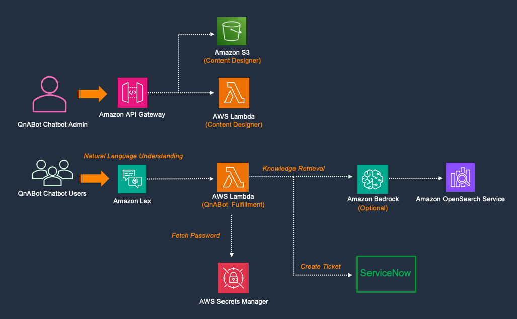
Integrate QnABot on AWS with ServiceNow
Go Here to Read this Fast! Integrate QnABot on AWS with ServiceNow


Originally appeared here:
Deploy large language models for a healthtech use case on Amazon SageMaker


Everything you’d ever want to know about a day in the life of a data professional!
Originally appeared here:
A Day in the Life of an Analytics Consultant in 2024
Go Here to Read this Fast! A Day in the Life of an Analytics Consultant in 2024

K-Nearest Neighbors is one of the most popular machine-learning algorithms out there. Its simplicity, versatility, and adaptability make it a common choice. But, why is it so popular? Why does it perform so well? This article peels back the layers of KNN, revealing how it works and why it’s a favored tool for many data scientists. We’ll look at its applications, and its math, we’ll build it from scratch, and discuss how, in a field driven by the latest technologies, KNN remains relevant and widely used.
Index
· 1: Understanding the Basics
∘ 1.1: What is K-Nearest Neighbors?
∘ 1.2: How Does KNN Work?
· 2: Implementing KNN
∘ 2.1: The Mathematics Behind KNN
∘ 2.2: Choosing the Right K Value
∘ 2.3: How to choose the right Distance Metric
· 3: KNN in Practice
∘ 3.1 KNN From Scratch in Python
∘ 3.2 Implementing KNN with Scikit-Learn
· 4: Advantages and Challenges
∘ 4.1 Benefits of Using KNN
∘ 4.2 Overcoming KNN Limitations
· 5: Beyond Basic KNN
∘ 5.1 Variants of KNN

The K-Nearest Neighbors algorithm works on a simple assumption: similar objects tend to be found near each other. It’s like when you’re in a huge library looking for books on, let’s say, baking. If you don’t have a guide, you’ll probably just grab books randomly until you find a cooking book, and then start grabbing books nearby as you hope they’re about baking because cookbooks are usually kept in the same spot.
KNN is like the memory whiz of machine learning algorithms. Instead of learning patterns and making predictions like many others do, KNN remembers every single detail of the training data. So, when you throw a new piece of data at it, it digs through everything it remembers to find the data points that are most similar to this new one. These similar points are its ‘nearest neighbors.’
To figure out which neighbors are closest, the algorithm measures the distance between the new data and everything it knows using methods like Euclidean or Manhattan distance. The choice of method matters a lot because it can change how KNN performs. For example, Euclidean distance works great for continuous data, while Manhattan distance is a go-to for categorical data.
After measuring the distances, KNN picks the ‘k’ closest ones. The ‘k’ here is important because it’s a setting you choose, and it can make or break the algorithm’s accuracy. If ‘k’ is too small, the algorithm can get too fixated on the noise in your data, which isn’t great. But if ‘k’ is too big, it might consider data points that are too far away, which isn’t helpful either.
For classification tasks, K-Nearest Neighbors looks at the most common class among these ‘k’ neighbors and goes with that. It’s like deciding where to eat based on where most of your friends want to go. For regression tasks, where you’re predicting a number, it calculates the average or sometimes the median of the neighbors’ values and uses that as the prediction.
What’s unique about KNN is it’s a ‘lazy’ algorithm, meaning it doesn’t try to learn a general pattern from the training data. It just stores the data and uses it directly to make predictions. It’s all about finding the nearest neighbors based on how you define ‘closeness,’ which depends on the distance method you use and the value of ‘k’ you set.

Step 1: Calculate Distance
Firstly, we calculate the distance between the current data point and all the data points in the training set. The purpose is to find the ‘k’ instances in the training set that are nearest to the query instance.
Here, we have a wide choice of distance functions we could use. But let’s stick to the three most popular ones for now: Euclidean distance, Manhattan distance, and Minkowski distance.
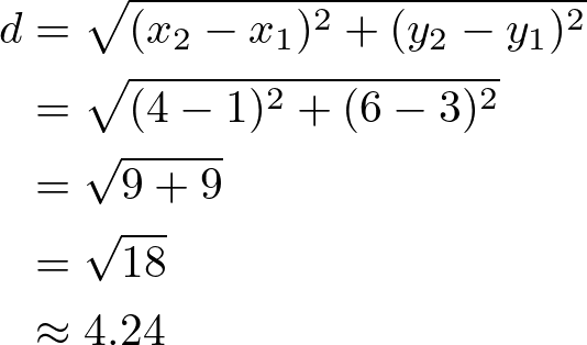
Euclidean Distance
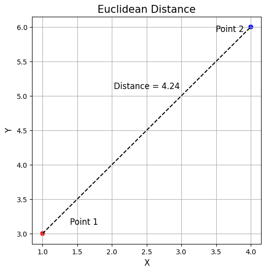
Used commonly for continuous data, it’s the straight-line distance between two points in Euclidean space.

In this equation:
In the image, this would be
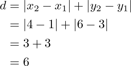
Manhattan Distance
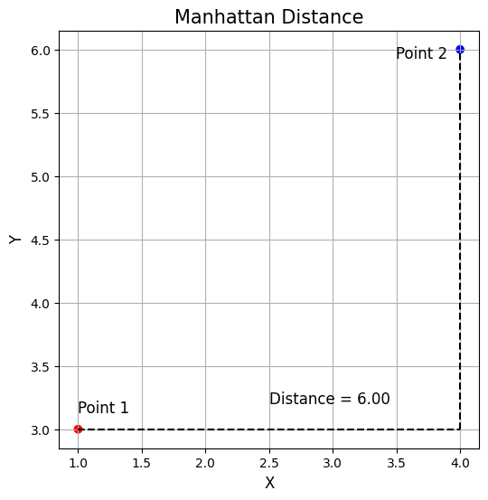
Also known as the city block distance, it is the sum of the absolute differences of their Cartesian coordinates. Unlike the straight-line distance measured by Euclidean distance, Manhattan distance calculates the distance traveled along axes at right angles. It’s preferred for categorical data.
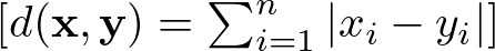
Following the example above this would be:
Minkowski Distance
It’s a generalization of both Euclidean and Manhattan distances. It introduces a parameter p that allows different distance metrics to be calculated. The Minkowski distance includes both the Euclidean distance and the Manhattan distance as special cases when p=2 and p=1, respectively.
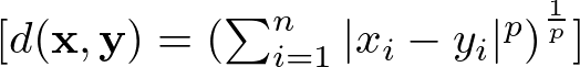
Here:
Step 2: Identify Nearest Neighbors
After calculating the distances, the algorithm sorts them and selects the ‘k’ smallest distances. This step identifies the ‘k’ nearest neighbors to the current data point.
Step 3: Aggregate Nearest Neighbors
For Classification KNN aggregates the class labels of the ‘k’ nearest neighbors to predict the class of the current data point. The most common class label among the ‘k’ nearest neighbors is chosen as the prediction.

where Cq is the predicted class for the current data point, and Cni is the class of the ‘k’ nearest neighbors.
For Regression KNN calculates the mean (or sometimes median) of the target values of the ‘k’ nearest neighbors to predict the value for the current data point.
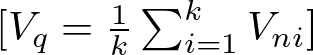
where Vq is the predicted value for the query instance, and Vni is the target value of the ‘k’ nearest neighbors.
Step 4: Predict the Outcome
Based on the aggregation in Step 3, KNN predicts the class (for classification tasks) or value (for regression tasks) of the query instance. This prediction is made without the need for an explicit model, as KNN uses the dataset itself and the distances calculated to make predictions.
Choosing the right number of neighbors, or ‘k’, in the K-Nearest Neighbors (KNN) algorithm is so important, that could be considered as one of the algorithm’s limitations, as a poor choice would likely lead to a poor performance. The perfect ‘k’ helps the model catch the real patterns in the data, while the wrong ‘k’ could lead to guesses that are off the mark. Fortunately, there are a few techniques we can use to better understand what ‘k’ to use.
Cross Validation
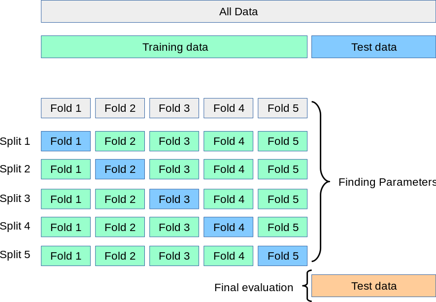
Think of this as trial runs. You divide your data into ‘k’ groups, for every run you use one group as a test and all the other ones to train the model. Using cross-validation avoids overfitting, and it’s likely to be a better representation of reality. Then, we test different k-values and pick the k which reports the best accuracy.
Error Rate Analysis
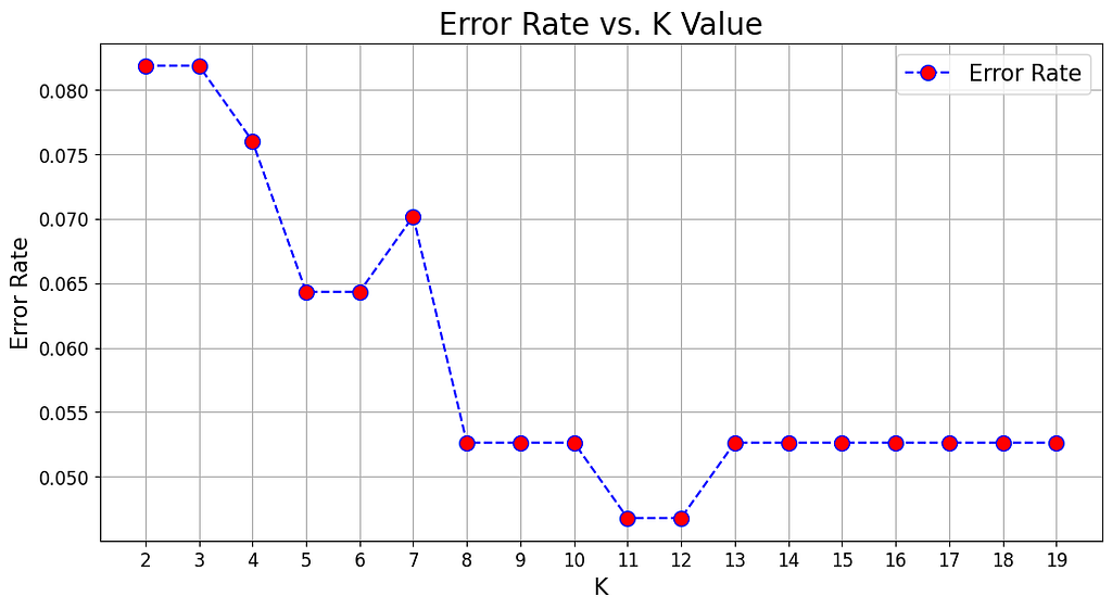
This is about drawing a graph of ‘how wrong your model gets’ against different ‘k’ values. You’re looking for the ‘k’ where things start to level off, showing you’re getting the most bang for your buck without the model’s performance going downhill. In the picture above 11 would be the best K to choose, as it gives the lowest error rate.
Knowing Your Field
This may sound obvious, but knowing what you’re studying can hint at the best ‘k’. If you know how your data tends to group or spread out, you can pick a ‘k’ that makes sense for the real-world scenario you’re trying to model.
Choosing the right distance metric is also a critical step in optimizing the KNN for specific datasets and problem domains. Using an analogy, it’s like choosing the right glasses to see the data clearly: the better the fit, the clearer you’ll see your ‘k’ nearest neighbors and the better your predictions will be.
To understand what’s the best distance to use, you should ask yourself the following questions:

1. What’s your data like?
Continuous vs. Categorical: If your data is all about numbers and measurements (continuous data), Euclidean distance is your go-to, because it measures straight lines between points. For data that’s more about categories (like types of fruit, where “apple” and “orange” aren’t on a scale), Hamming distance, which checks if features match, makes more sense.
Scale of Features: Look out for different scales in your dataset. If you don’t adjust for this, your distances could be thrown off, making some features louder than others. Normalize your data or switch to Manhattan distance, which isn’t as thrown off by different scales.
2. How big is your data?
When your dataset is really wide (lots of features), traditional ideas of closeness get wonky, and everything starts to seem far apart. Here, reducing dimensions or picking metrics suited for the big stage, like cosine similarity for text, can keep things in perspective.
3. How is your data spread out?
The way your data is distributed matters. If outliers are a big deal in your dataset, Manhattan distance might be your ally since it doesn’t get as shaken up by extreme values compared to Euclidean distance.
4. Need for speed?
Some distance metrics are computationally more intensive than others. Metrics like Manhattan distance can be computationally more efficient than Euclidean distance in certain implementations since it lacks the square root operation.
Lastly, don’t marry the first metric you meet. Play the field, try different metrics, and see which one makes your model the happiest through cross-validation.
Now let’s see what we described in math terms looks like in Python code. Let’s start by defining the whole class and then break it down into smaller pieces:
import numpy as np
from collections import Counter

class KNN:
    def __init__(self, k=3, distance_metric='euclidean'):
        self.k = k
        self.distance_metric = distance_metric

    def _euclidean_distance(self, x1, x2):
        """
        Compute the Euclidean distance between two vectors

        Parameters
        ----------
        x1 : array-like
            A vector in the feature space
        x2 : array-like
            A vector in the feature space

        Returns
        -------
        float
            The Euclidean distance between x1 and x2
        """
        return np.sqrt(np.sum((x1 - x2)**2))

    def _manhattan_distance(self, x1, x2):
        """
        Compute the Manhattan distance between two vectors

        Parameters
        ----------
        x1 : array-like
            A vector in the feature space
        x2 : array-like
            A vector in the feature space

        Returns
        -------
        float
            The Manhattan distance between x1 and x2
        """
        return np.sum(np.abs(x1 - x2))

    def _minkowski_distance(self, x1, x2):
        """
        Compute the Minkowski distance between two vectors

        Parameters
        ----------
        x1 : array-like
            A vector in the feature space
        x2 : array-like
            A vector in the feature space

        Returns
        -------
        float
            The Minkowski distance between x1 and x2
        """
        return np.sum(np.abs(x1 - x2)**self.k) ** (1/self.k)

    def fit(self, X, y):
        """
        Fit the model using X as training data and y as target values

        Parameters
        ----------
        X : array-like
            Training data
        y : array-like
            Target values
        """
        self.X_train = X
        self.y_train = y

    def predict(self, X):
        """
        Predict the class labels for the provided data

        Parameters
        ----------
        X : array-like
            Data to be used for prediction

        Returns
        -------
        array-like
            Predicted class labels
        """
        predicted_labels = [self._predict(x) for x in X]
        return np.array(predicted_labels)

    def _predict(self, x):
        """
        Predict the class label for a single sample

        Parameters
        ----------
        x : array-like
            A single sample

        Returns
        -------
        int
            The predicted class label
        """
        # Compute distances between x and all examples in the training set
        if self.distance_metric == 'euclidean':
            distances = [self._euclidean_distance(x, x_train) for x_train in self.X_train]
        elif self.distance_metric == 'manhattan':
            distances = [self._manhattan_distance(x, x_train) for x_train in self.X_train]
        elif self.distance_metric == 'minkowski':
            distances = [self._minkowski_distance(x, x_train) for x_train in self.X_train]
        else:
            raise ValueError("Invalid distance metric. Choose from 'euclidean', 'manhattan', 'minkowski'.")

        # Sort by distance and return indices of the first k neighbors
        k_indices = np.argsort(distances)[:self.k]
        # Extract the labels of the k nearest neighbor training samples
        k_nearest_labels = [self.y_train[i] for i in k_indices]
        # return the most common class label
        most_common = Counter(k_nearest_labels).most_common(1)
        return most_common[0][0]
Initialization
def __init__(self, k=3, distance_metric='euclidean'):
        self.k = k
        self.distance_metric = distance_metric
The KNN class first initializes two variables: k, and the distance metric. Here ‘k’, is the number of k-neighbors we want to use for the model, and the distance metric is a text field to specify what metric we want to use to compute the distance. In this example, we present three options — Euclidean, Manhattan, and Minkowski distance — but feel free to experiment with more distances.
Distance Methods
def _euclidean_distance(self, x1, x2):
        return np.sqrt(np.sum((x1 - x2)**2))

def _manhattan_distance(self, x1, x2):
        return np.sum(np.abs(x1 - x2))

def _minkowski_distance(self, x1, x2):
        return np.sum(np.abs(x1 - x2)**self.k) ** (1/self.k)
Next, we define three methods that will calculate the specified distance. They are just the Pythonic expression of the math formulas we defined before. Nothing fancy, and pretty straightforward.
Fit Method
def fit(self, X, y):
        self.X_train = X
        self.y_train = y
The fit method stores the X, and y, as class variables, which will later be called by the predict method.
_predict Method
def _predict(self, x):
        # Compute distances between x and all examples in the training set
        if self.distance_metric == 'euclidean':
            distances = [self._euclidean_distance(x, x_train) for x_train in self.X_train]
        elif self.distance_metric == 'manhattan':
            distances = [self._manhattan_distance(x, x_train) for x_train in self.X_train]
        elif self.distance_metric == 'minkowski':
            distances = [self._minkowski_distance(x, x_train) for x_train in self.X_train]
        else:
            raise ValueError("Invalid distance metric. Choose from 'euclidean', 'manhattan', 'minkowski'.")

        # Sort by distance and return indices of the first k neighbors
        k_indices = np.argsort(distances)[:self.k]
        # Extract the labels of the k nearest neighbor training samples
        k_nearest_labels = [self.y_train[i] for i in k_indices]
        # return the most common class label
        most_common = Counter(k_nearest_labels).most_common(1)
        return most_common[0][0]
This is the core method of the class. It first accesses the distance metric variable we initialized at the beginning of the class, then calculates the distances between the data point we want to predict and all the data points in the training set.
After calculating the distances, we sort them by ascending order and return the first k indices, where k is the number of neighbors we initialized at the beginning of the class.
Lastly, we retrieve the target values in the training dataset associated with the indices and return the most common value.
Note, that this last step would be different in case of regression, as would calculate the mean or median instead.
predict Method
def predict(self, X):
        predicted_labels = [self._predict(x) for x in X]
        return np.array(predicted_labels)
Finally, we define the predict method, which is a wrapper of the previous _predict method. What this method does is call the _predict method on all the observations in X, which are the observations we want to predict. Lastly, it returns all the predictions stored in a numpy array.
And, that’s it! Pretty cool, right? Very simple algorithm, but still very powerful.
For the full code, and a practical implementation look at this Jupyter Notebook:
models-from-scratch-python/KNN/demo.ipynb at main · cristianleoo/models-from-scratch-python
As I usually say in my articles, the code above is likely what you don’t want to use in production, as I created it just for educational purposes. Instead, we can take advantage of the great sci-kit learn library, which offers a better and more efficient version of the algorithm, and we just a few lines of code.
from sklearn import datasets
from sklearn.model_selection import train_test_split
from sklearn.preprocessing import StandardScaler
from sklearn.neighbors import KNeighborsClassifier
from sklearn.metrics import accuracy_score

# Load iris dataset
iris = datasets.load_iris()
X = iris.data
y = iris.target

# Split the data into training and test sets
X_train, X_test, y_train, y_test = train_test_split(X, y, test_size=0.2, random_state=42)

# Standardize the features
sc = StandardScaler()
X_train_std = sc.fit_transform(X_train)
X_test_std = sc.transform(X_test)

# Create KNN classifier
knn = KNeighborsClassifier(n_neighbors=3)

# Fit the classifier to the data
knn.fit(X_train_std, y_train)

# Predict the labels of the test set
y_pred = knn.predict(X_test_std)

# Print the accuracy of the classifier
print(f'Accuracy: {accuracy_score(y_test, y_pred):.2%}')
# Accuracy 100.00%
For this example, we are using the Iris dataset, and defining a KNN with 3 Neighbors, and distance method Minkowski with p=2, which is the default distance method for KNN in sci-kit learn. As we can see the code works similarly to what we built from scratch.
Now feel free to use this code, and play with it.
The K-Nearest Neighbors (KNN) algorithm, despite its simplicity, offers several compelling advantages that make it a valuable tool for both classification and regression tasks in machine learning. Its intuitive approach, based on the principle that similar instances tend to be near each other, allows it to perform remarkably well across a wide range of applications. Here, we explore the key benefits of using KNN:
Simple and Intuitive
KNN wins big points for being straightforward. It’s the kind of algorithm that doesn’t need you to be a machine-learning wizard to use effectively. The whole concept of looking for the nearest neighbors based on how close they are is something anyone can understand. This makes this algorithm a friendly starting point for beginners.
No Assumptions About Data
Unlike many machine learning algorithms that make assumptions about the distribution of the data, KNN is non-parametric. This means it makes no prior assumptions about the form of the data, allowing it to be effective in scenarios where the data distribution is unknown or the relationship between variables is complex.
Adaptability
Adjustments to the number of neighbors (‘k’) or the choice of distance metric can significantly change the algorithm’s behavior, allowing for fine-tuning to specific datasets or problem characteristics. This adaptability extends to its capacity to deal with changes in the data, as KNN naturally incorporates new information during prediction without needing to be retrained.
Robustness to Noisy Data
In a perfect world, data would be clean and tidy. In the real world, not so much. KNN is pretty good at dealing with messy, noisy data. Since it looks at several neighbors to make a decision, a few oddballs here and there won’t throw it off track. Using a smart voting or averaging system can help make sure the reliable data gets more say.
While K-Nearest Neighbors is a go-to for its straightforward approach and adaptability, it’s not without its flaws. Let’s walk through some of the main challenges you might bump into and talk about how to tackle them head-on.
Computational Complexity
The biggest gripe with KNN is how much it demands in terms of computation, especially with hefty datasets. It’s like trying to remember every person you’ve ever met — the more people, the harder it gets.
To overcome this, try to use efficient data structures such as KD-Trees or Ball Trees to reduce search time for nearest neighbors. Also, consider applying dimensionality reduction techniques like Principal Component Analysis (PCA) to trim down the excess features, making the distance calculation quicker and less of a headache.
For a comprehensive guide on PCA consider looking at this article:
Principal Component Analysis (PCA): From Scratch in Python
Sensitivity to Irrelevant Features
KNN treats every feature like it’s equally important, which isn’t always the case.
Here, two approaches you may follow are feature selection and scaling. Use feature selection to spotlight the features that matter, and scale your features so they all have an equal shot at influencing the outcome.
Handling of Categorical Data
KNN assumes numerical data for distance calculation, making the direct application to categorical data challenging.
Because of this, it’s important to encode categorical data using techniques like one-hot encoding before applying KNN. Also, use distance metrics specifically designed for categorical data, such as the Hamming distance.
Data Imbalance
In a dataset where one class overshadows the others, KNN might get a little biased towards the more common class.
In this case, we can trick KNN, and use one of its variants: weighted KNN, where the votes of the nearest neighbors are weighted by their distance, giving more influence to the closer neighbors.
Another approach would be applying sampling techniques to balance the dataset, such as oversampling the minority class or undersampling the majority class.
The K-Nearest Neighbors algorithm, while powerful in its standard form, has inspired several variants designed to address its limitations and adapt to specific challenges. These variations extend KNN’s applicability and efficiency, making it even more versatile across a wider range of datasets and problem settings. Here, we explore some of the notable variants of the KNN algorithm.
Weighted KNN
This twist on KNN doesn’t treat all neighbors equally. Instead, it gives more say to the ones closer to the point you’re looking at. Think of it as paying more attention to your close friends’ opinions than acquaintances when making a decision. This can make your predictions sharper, especially when some neighbors should matter more than others.
Radius-Based KNN
Instead of counting neighbors, this version draws a circle (or sphere) of a fixed size around your point and considers anyone inside that space. It’s a bit like deciding who gets to come to your party based on how close they live. This is super handy for areas where your data points are all over the place in terms of how close together they are.
KD-Trees and Ball Trees
These are fancy ways of organizing your data so you can find your nearest neighbors without having to check every single point. Imagine organizing your bookshelf so you can instantly grab books from a certain genre without looking through every book. It’s a game-changer for working with big datasets where finding neighbors the old-fashioned way would take too long.
Locally Sensitive Hashing (LSH) for KNN
LSH is like a shortcut for finding neighbors by grouping similar items into buckets. It’s a bit like sorting people into groups based on their interests so you can quickly find someone to chat with. This method can speed things up a lot, especially with huge datasets, but it’s a bit of a trade-off because you might not get as precise results.
KNN with Feature Learning
Some KNN variations are all about getting smarter at figuring out which features (or characteristics) of your data are important. Using tools like autoencoders or deep metric learning, KNN can better see which data points are truly close together. It’s akin to learning to read between the lines to understand what brings people together.
KNN for Imbalanced Data
When your data is lopsided, with way more examples of one thing than another, these KNN versions tweak how they count votes or choose neighbors to make sure the underdog gets a fair shake. It’s like making sure everyone in a small town gets heard, not just the folks who talk the loudest.
The magic of KNN lies in how it uses the idea of “nearness” to make predictions, a concept as old as time but incredibly effective for everything from sorting photos to predicting stock trends. Its flexibility is on full display across different sectors like healthcare, finance, and cybersecurity, where it’s not just about tagging data points but solving complex problems that matter.
We’ve also seen the different flavors of KNN that can be customized for specific challenges, whether it’s dealing with vast amounts of data or making sure smaller voices aren’t drowned out in imbalanced datasets. This adaptability is what makes KNN such a valuable tool in the toolbox of machine learning.
Of course, KNN isn’t perfect. It can be a bit of a resource hog, requires a bit of tuning to get ‘k’ and the distance metric just right, and doesn’t always play nice with irrelevant features or data of varying scales. But the good news is, that we’ve got strategies to tackle these issues, from smart data prep to using clever data structures, paving the way to make the most of what KNN has to offer.
You made it to the end. Congrats! I hope you enjoyed this article, if so consider leaving a like and following me, as I will regularly post similar articles. My goal is to recreate all the most popular algorithms from scratch and make machine learning accessible to everyone.
The Math Behind KNN was originally published in Towards Data Science on Medium, where people are continuing the conversation by highlighting and responding to this story.
Originally appeared here:
The Math Behind KNN
