
Originally appeared here:
Measuring AI’s Creativity with Visual Word Puzzles
Go Here to Read this Fast! Measuring AI’s Creativity with Visual Word Puzzles
Explore the potentials and constraints of LangChain for customer analytics, accompanied by practical implementation codes
Originally appeared here:
Performing Customer Analytics with LangChain and LLMs
Go Here to Read this Fast! Performing Customer Analytics with LangChain and LLMs

Originally appeared here:
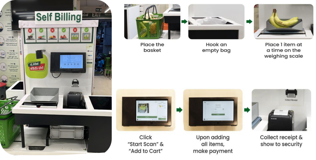
How BigBasket improved AI-enabled checkout at their physical stores using Amazon SageMaker

Originally appeared here:
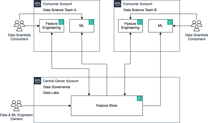
Amazon SageMaker Feature Store now supports cross-account sharing, discovery, and access

K-means clustering is a staple in machine learning for its straightforward approach to organizing complex data. In this article we’ll explore the core of the algorithm. We will delve into its applications, dissect the math behind it, build it from scratch, and discuss its relevance in the fast-evolving field of data science.
Index
· 1: Understanding the Basics
∘ 1.1: What is K-Means Clustering?
∘ 1.2: How Does K-Means Work?
· 2: Implementing K-Means
∘ 2.1: The Mathematics Behind K-Means
∘ 2.2: Choosing the Optimal Number of Clusters
· 3: K-Means in Practice
∘ 3.1 K-Means From Scratch in Python
∘ 3.2 Implementing K-Means with Scikit-Learn
· 4: Advantages and Challenges
∘ 4.1 Benefits of Using K-Means
∘ 4.2 Overcoming K-Means Limitations
· 5: Beyond Basic K-Means
∘ 5.1 Variants of K-Means
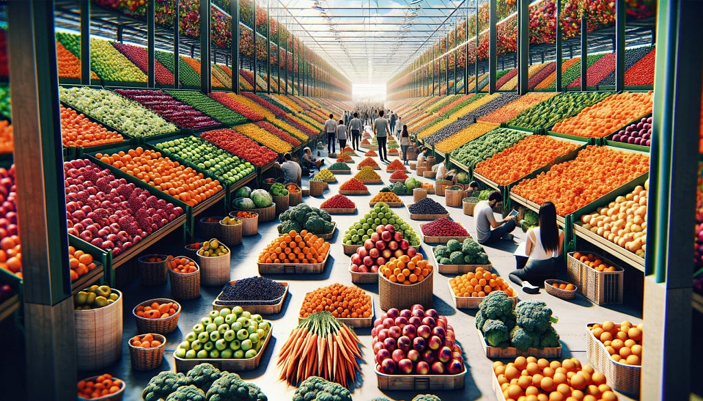
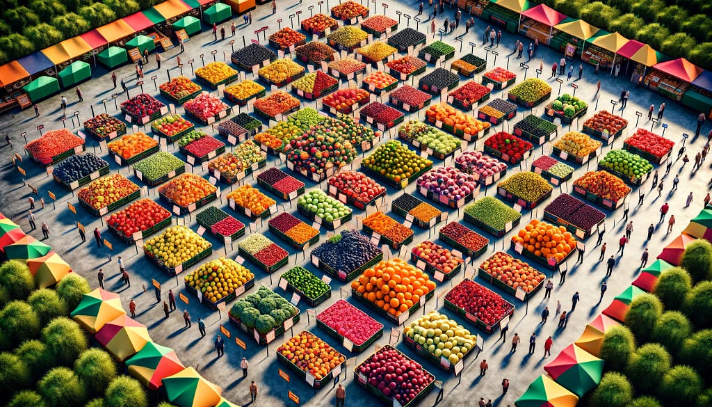
Imagine you’re at a farmer’s market with a bunch of fruits and veggies that you need to sort out. You want to organize them so all the apples, oranges, and carrots are hanging out with their kind. This task is a lot like what K-Means Clustering does in data science.
So, what’s K-Means Clustering? It’s a technique used to naturally group data. Think of it as a way to sort unlabeled data into different groups or clusters. Each cluster is a bunch of data points that are more alike to each other than to those in other groups. The “K” in K-Means? It represents the number of groups you think there should be.
Now, keep in mind the farmer’s market example, and let’s try to dive deep a bit more into K-means mechanisms.
Think of K-Means as setting up the initial fruit stands (centroids) in our market. It randomly picks a few spots (data points) to place these stands. The number of stands you decide to set up is the “K” in K-Means, and this number depends on how many different types of produce (groups) you think you have.
Now, K-Means takes each fruit and veggie (data point) and figures out which stand (centroid) it belongs to based on how close it is. It’s like each apple, orange, or carrot choosing the closest stand to hang out at, forming little groups around them.
After all the produce has found a stand, K-Means checks if the stands are in the best spots. It does this by finding a new spot for each stand based on the average position of all the produce grouped around them. It’s similar to moving the stands to the exact middle of each produce group to make sure they’re truly at the heart of the action.
This process of sorting produce and adjusting stands keeps going. Fruits and veggies might move to a different stand if they find one closer, and the stands might shift positions to better represent their groups. This cycle continues until the stands and their produce groups don’t change much anymore. That’s when K-Means knows the market is perfectly organized, and every piece of produce is of its kind.
What you end up with are nicely organized stands (clusters) with fruits and veggies grouped around them. Each stand represents a type of produce, showing you how your market (data) can be divided into distinct sections (categories) based on similarities.
Let’s put on our math hats for a moment and peek into the engine room of the K-Means algorithm to see what makes it tick. K-Means is all about finding the sweet spot:
the optimal placement of centroids that minimizes the distance between points in a cluster and their central point.
Here’s how the math plays out:
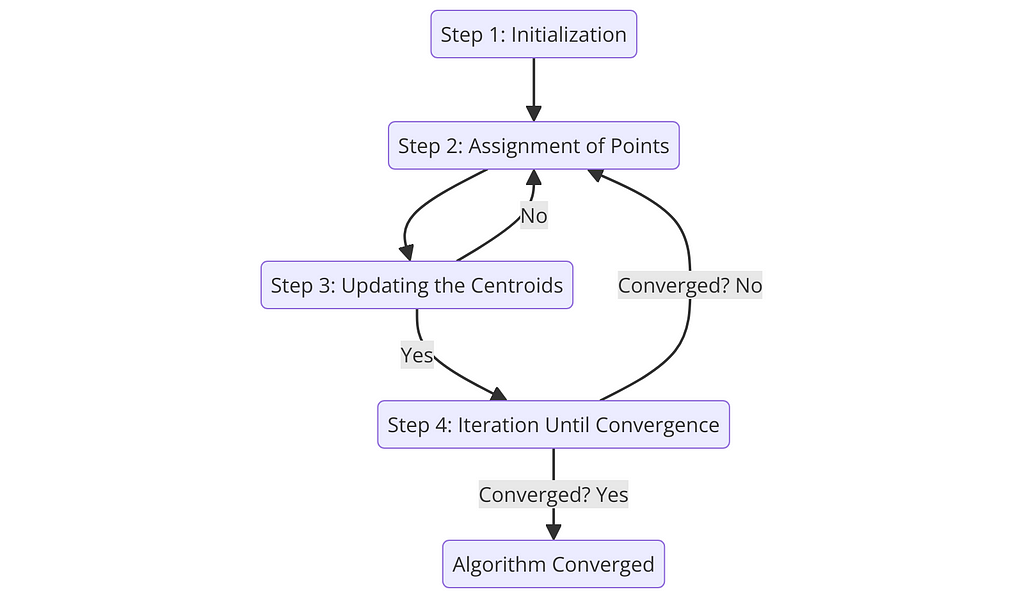
Step 1: Initialization
Initially, K-Means needs to decide where to start, choosing k initial centroids (μ1,μ2,…,μk) from the dataset. This can be done randomly or more strategically with methods like K-Means++, which we will cover later.
While no specific formula is used here, the choice of initial centroids can significantly affect the outcome. But don’t worry, because, in the next section, we will guide you through the best tips to choose the optimal k.
Step 2: Assignment of Points to Closest Centroid
NeXT, each data point x is assigned to the nearest centroid, forming k clusters, where the “nearest” centroid is determined by the minimum distance between the point and all centroids.
Here, the distance d between a point x and a centroid μi is typically calculated using the Euclidean distance:
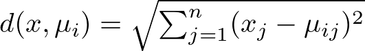
where xj and μij are the j-th dimensions of point x and centroid μi, respectively. Now, while Euclidean distance is the most popular choice for K-Means, you could explore its application with more distances. However, keep in mind that Euclidean distance is usually the suggested choice for optimal performance, whereas other variances of the algorithm are more flexible to different distance methods. Look at the subsection 2.1 of my previous article about K-Nearest Neighbors to know more about distance methods:
The Math Behind K-Nearest Neighbors
Keeping the Euclidean distance in mind, let’s see how the algorithm assigns a point x to the cluster Ci:

Here’s what it means:
The condition d(x,μi) ≤ d(x,μj) ∀ j, 1≤j≤k specifies that a point x is assigned to the cluster Ci if and only if the distance from x to the centroid μi of Ci is less than or equal to its distance from x to the centroids μj of all other clusters Cj, for every j from 1 to k.
In simpler terms, the formula says:
Look at all the clusters and their centers (centroids). Now, find which centroid is closest to point x. Whichever cluster has this closest centroid, that’s the cluster x belongs to.
This step ensures that each point is assigned to the cluster with the nearest centroid, minimizing within-cluster distances and making the clusters as tight and homogenous as possible.
Step 3: Updating the Centroids
After all points have been assigned to clusters, the positions of the centroids are recalculated to be at the center of their respective clusters.
The new position μi′ of centroid μi is calculated as the mean of all points assigned to cluster Ci:
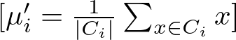
where ∣Ci∣ is the number of points in cluster Ci, and the summation aggregates the positions of all points in the cluster.
Step 4: Iteration Until Convergence
The assignment and update steps (Steps 2 and 3) are repeated until the centroids no longer change significantly, indicating that the algorithm has converged.
Here, convergence is typically assessed by measuring the change in centroid positions between iterations. If the change falls below a predetermined threshold, the algorithm stops.
In the context of the K-Means algorithm, there isn’t a single, universally defined formula for convergence that applies in all cases. Instead, convergence is determined based on the algorithm’s behavior over successive iterations, specifically whether the centroids of the clusters stop changing significantly.
However, a common way to assess convergence is by looking at the change in the within-cluster sum of squares (WCSS) or the positions of the centroids between iterations. Here, we set a threshold for changes in the centroid positions or the WCSS. If the change falls below this threshold from one iteration to the next, the algorithm can be considered to have converged. This can be expressed as:
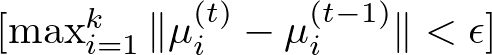
where:
Deciding on the right number of clusters, k, in K-Means clustering is more art than science. It’s like Goldilocks trying to find the bed that’s just right, with not too many clusters to overcomplicate things, and not too few to oversimplify. Here’s how you can find that sweet spot:
The Elbow Method
One popular technique is the Elbow Method. It involves running K-Means several times, each time with a different number of clusters, and then plotting the Within-Cluster Sum of Squares (WCSS) against the number of clusters. WCSS measures how tight your clusters are, with lower values indicating that points are closer to their respective centroids.
The formula for calculating WCSS is :

Here’s a breakdown of this formula:
The WCSS is essentially a sum of these squared distances for all points in each cluster, aggregated across all k clusters. A lower WCSS value indicates that points are on average closer to their cluster centroids, suggesting tighter and possibly more meaningful clusters.
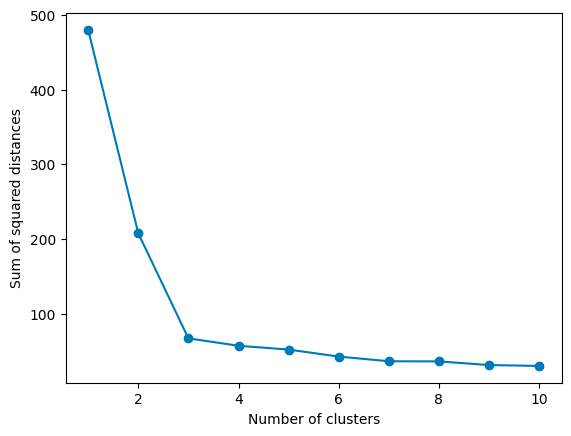
As you increase k, WCSS decreases because the points are closer to centroids. However, there’s a point where adding more clusters doesn’t give you much bang for your buck. This point, where the rate of decrease sharply changes, looks like an elbow on the graph. In the graph above, the elbow point is 3, as the rate of decrease slows down significantly afterward. That’s your Goldilocks k:
Elbow point ≈ Optimal k
The Silhouette Method
Another approach is the Silhouette Method, which evaluates how similar an object is to its cluster compared to other clusters. The silhouette score ranges from -1 to 1, where a high value indicates that the object is well-matched to its cluster and poorly matched to neighboring clusters.
The formula for calculating the Silhouette Score for a single data point is:
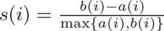
Then, we take the average silhouette score for the dataset, which is calculated by averaging the silhouette scores of all points. In mathematical terms:

where N is the total number of points in the dataset.
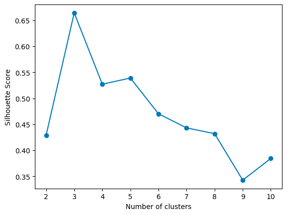
For each k, calculate the average silhouette score of all points. The k that gives you the highest average silhouette score is considered the optimal number of clusters. It’s like finding the party where everyone feels they fit in best. In the graph above, the highest score is given by 3 clusters.
Max average silhouette score → Optimal k
K-Means++
Means++ is an algorithm for choosing the initial values (or “seeds”) for the K-Means clustering algorithm. The standard K-Means algorithm starts with a random selection of centroids, which can sometimes result in poor convergence speed and suboptimal clustering. K-Means++ addresses this by spreading out the initial centroids before proceeding with the standard K-Means optimization iterations.
It begins by randomly selecting the first centroid from the dataset. Then, for each subsequent centroid, K-Means++ chooses data points as new centroids with a probability proportional to their squared distance from the nearest existing centroid. This step increases the chances of selecting centroids that are far away from each other, reducing the likelihood of poor clustering. This process is repeated until all k centroids are chosen.
Lastly, once the initial centroids are selected using the K-Means++ approach, continue with the standard K-Means algorithm to adjust the centroids and assign points to clusters.
In this post, I won’t delve deep into K-Means++ math, but expect it in a new post. In the meantime, you could read the following article for a better understanding:
k-means++: The Advantages of Careful Seeding
As I like to do in this “Machine Learning From Scratch” series, let’s now recreate a simpler version of the algorithm from scratch. Let’s first look at the whole code:
class KMeans:
    def __init__(self, K, max_iters=100, tol=1e-4):
        """
        Constructor for KMeans class

        Parameters
        ----------
        K : int
            Number of clusters
        max_iters : int, optional
            Maximum number of iterations, by default 100
        tol : float, optional
            Tolerance to declare convergence, by default 1e-4
        """
        self.K = K
        self.max_iters = max_iters
        self.tol = tol
        self.centroids = None
        self.labels = None
        self.inertia_ = None

    def initialize_centroids(self, X):
        """
        Initialize centroids

        Parameters
        ----------
        X : array-like
            Input data

        Returns
        -------
        array-like
            Initial centroids
        """
        # Simple random initialization, consider k-means++ for improvement
        indices = np.random.permutation(X.shape[0])
        centroids = X[indices[:self.K]]
        return centroids

    def compute_centroids(self, X, labels):
        """
        Compute centroids

        Parameters
        ----------
        X : array-like
            Input data
        labels : array-like
            Cluster labels

        Returns
        -------
        array-like
            Updated centroids
        """
        centroids = np.zeros((self.K, X.shape[1]))
        for k in range(self.K):
            if np.any(labels == k):
                centroids[k] = np.mean(X[labels == k], axis=0)
            else:
                centroids[k] = X[np.random.choice(X.shape[0])]
        return centroids

    def compute_distance(self, X, centroids):
        """
        Compute distances between data points and centroids

        Parameters
        ----------
        X : array-like
            Input data
        centroids : array-like
            Centroids

        Returns
        -------
        array-like
            Distances
        """
        distances = np.zeros((X.shape[0], self.K))
        for k in range(self.K):
            distances[:, k] = np.linalg.norm(X - centroids[k], axis=1) ** 2
        return distances

    def find_closest_cluster(self, distances):
        """
        Find the closest cluster for each data point

        Parameters
        ----------
        distances : array-like
            Distances

        Returns
        -------
        array-like
            Cluster labels
        """
        return np.argmin(distances, axis=1)

    def fit(self, X):
        """
        Fit the model

        Parameters
        ----------
        X : array-like
            Input data
        """
        self.centroids = self.initialize_centroids(X)
        for i in range(self.max_iters):
            distances = self.compute_distance(X, self.centroids)
            self.labels = self.find_closest_cluster(distances)
            new_centroids = self.compute_centroids(X, self.labels)
            # Compute inertia (sum of squared distances)
            inertia = np.sum([distances[i, label] for i, label in enumerate(self.labels)])
            # Check for convergence: if the centroids don't change much (within tolerance)
            if np.allclose(self.centroids, new_centroids, atol=self.tol) or inertia <= self.tol:
                break
            self.centroids = new_centroids
        self.inertia_ = inertia

    def predict(self, X):
        """
        Predict the closest cluster for each data point

        Parameters
        ----------
        X : array-like
            Input data

        Returns
        -------
        array-like
            Cluster labels
        """
        distances = self.compute_distance(X, self.centroids)
        return self.find_closest_cluster(distances)
Let’s break down each part of the class to explain its functionality:
def __init__(self, K, max_iters=100, tol=1e-4):
        self.K = K
        self.max_iters = max_iters
        self.tol = tol
        self.centroids = None
        self.labels = None
        self.inertia_ = None
This method initializes a new instance of the KMeans class.
Here, the parameters are:
We also initialize a few attributes to None:
2. initialize_centroids and compute_centroids Methods:
def initialize_centroids(self, X):
        # Simple random initialization, consider k-means++ for improvement
        indices = np.random.permutation(X.shape[0])
        centroids = X[indices[:self.K]]
        return centroids

    def compute_centroids(self, X, labels):
        centroids = np.zeros((self.K, X.shape[1]))
        for k in range(self.K):
            if np.any(labels == k):
                centroids[k] = np.mean(X[labels == k], axis=0)
            else:
                centroids[k] = X[np.random.choice(X.shape[0])]
        return centroids
First, we initialize the centroids randomly from the data points, by randomly permuting the indices of the input data and selecting the first K as the initial centroids. As we mentioned before, a random selection is one of the possible centroid initializations, you could go ahead and experiment with more techniques to see how this affects the performance of the model.
Then, we compute the new centroids as the mean of the data points assigned to each cluster. Here, if a cluster ends up with no points, a random data point from X is chosen as the new centroid for that cluster.
3. compute_distance and find_closest_clusterMethod:
def compute_distance(self, X, centroids):
        distances = np.zeros((X.shape[0], self.K))
        for k in range(self.K):
            distances[:, k] = np.linalg.norm(X - centroids[k], axis=1) ** 2
        return distances

    def find_closest_cluster(self, distances):
        return np.argmin(distances, axis=1)
We define the method to calculate the squared Euclidean distance between each data point and each centroid, which returns an array where each element contains the squared distances from a data point to all centroids.
Then, we assign each data point to the closest cluster based on the computed distances. The output of the operation consists of an array of labels indicating the closest cluster for each data point.
4. fit and predict Method:
def fit(self, X):
        self.centroids = self.initialize_centroids(X)
        for i in range(self.max_iters):
            distances = self.compute_distance(X, self.centroids)
            self.labels = self.find_closest_cluster(distances)
            new_centroids = self.compute_centroids(X, self.labels)
            # Compute inertia (sum of squared distances)
            inertia = np.sum([distances[i, label] for i, label in enumerate(self.labels)])
            # Check for convergence: if the centroids don't change much (within tolerance)
            if np.allclose(self.centroids, new_centroids, atol=self.tol) or inertia <= self.tol:
                break
            self.centroids = new_centroids
        self.inertia_ = inertia

    def predict(self, X):
        distances = self.compute_distance(X, self.centroids)
        return self.find_closest_cluster(distances)
Now we build the core method of this class: the fit method, which first initializes the centroids, and iterates up to max_iters times, where in each iteration:
Lastly, we predict the closest cluster for each point in a new dataset, using the predict method.
You can find the whole code and a practical implementation in this Jupyter Notebook:
models-from-scratch-python/K-Means/demo.ipynb at main · cristianleoo/models-from-scratch-python
Ok, now you have a solid understanding of what the algorithm does, and you can recreate the algorithm from scratch. Pretty cool right? Well, you won’t be using that code anytime soon, as our friend Scikit Learn already provides a much more efficient implementation of K-Means, which only takes a few lines of code. Here, we can use variations of K-Means only by specifying a parameter. Let’s look at one implementation of it.
from sklearn.cluster import KMeans
from sklearn.datasets import make_blobs

# Generate a synthetic dataset
X, y_true = make_blobs(n_samples=300, centers=3, cluster_std=0.60, random_state=0)

# Initialize and fit KMeans
kmeans = KMeans(n_clusters=3, max_iter=100, tol=1e-4)
kmeans.fit(X)

# Predict the cluster labels
labels = kmeans.predict(X)

# Print the cluster centers
print("Cluster centers:n", kmeans.cluster_centers_)
We first import KMeans from scikit-learn, and make_blobs is a function to generate synthetic datasets for clustering. We generate a synthetic dataset with 300 samples, 3 centers (clusters), and a standard deviation of 0.60 for each cluster. The random_state parameter is used to ensure that the results are reproducible.
We initialize the KMeans algorithm with 3 clusters (n_clusters=3), a maximum of 100 iterations (max_iter=100), and a tolerance of 1e-4 (tol=1e-4). The tolerance is the threshold to declare convergence — if the change in the within-cluster sum of squares (inertia) is less than this value, the algorithm will stop.
We fit the KMeans algorithm to our data using the fit method. This is where the actual clustering happens. We predict the cluster labels for our data using the predict method. This assigns each data point to the nearest cluster.
At this point, you probably have an idea of why K-Means is so popular, but let’s make sure you know when to consider K-Means for your data science journey:
Simplicity and Ease of Implementation
First off, K-Means is straightforward. It doesn’t ask for much, just the data and the number of clusters k you’re aiming for. This simplicity makes it super approachable, even for beginners in the data science field.
Efficiency at Scale
K-Means is pretty efficient, especially with large datasets. It’s got a way of cutting through data to find patterns without needing a supercomputer to do its thing. This efficiency makes it a practical choice for real-world applications where time and resources are of the essence.
Good for Pre-Processing and Simplification
The algorithm can also be a great pre-processing step. By clustering your data first, you can simplify complex problems, reduce dimensionality, or even improve the performance of other algorithms that you might run afterward.
Discovering Patterns and Insights
It can help uncover hidden structures that might not be immediately obvious, providing valuable insights into the nature of the data. This can inform decision-making, and strategy development, and even lead to discoveries within the data.
Easy Interpretation of Results
The results from K-Means are pretty straightforward to interpret. Clusters are defined clearly, and each data point is assigned to a specific group. This clarity can be particularly beneficial when explaining outcomes to stakeholders who might not have a deep technical background.
While K-Means clustering is a powerful tool for data analysis, it’s not without its quirks and challenges. Here’s a look at some common issues and strategies for addressing them:
Sensitivity to Initial Centroids
One of the main challenges with K-Means is that it’s quite sensitive to the initial placement of centroids. Random initialization can lead to suboptimal clustering or different results each time you run the algorithm.
Think about using the K-Means++ technique for initializing centroids. It’s a smarter way to start the clustering process, reducing the chances of poor outcomes by spreading out the initial centroids.
Fixed Number of Clusters
Deciding on the number of clusters k in advance can be tricky. Choose wrong, and you might end up forcing your data into too many or too few clusters.
As we said before, experimenting with methods like the Elbow Method and the Silhouette Score to find a suitable k. These approaches can provide more insight into the optimal number of clusters for your data.
Difficulty with Non-Spherical Clusters
A spherical cluster is one where the data points are roughly equidistant from the cluster’s center, resulting in a shape that is, in a multidimensional space, spherical or circular.
K-Means assumes that clusters are spherical and of similar size, which isn’t always the case in real-world data. This assumption can lead to less accurate clustering when the true clusters have irregular shapes.
In this case, consider using clustering algorithms designed for complex cluster shapes, such as Spectral Clustering or DBSCAN.
Sensitivity to Scale and Outliers
The performance of K-Means can be significantly affected by the scale of the data and the presence of outliers. Large-scale differences between features can skew the clustering, and outliers can pull centroids away from the true cluster center.
As usual, make sure to normalize the features to ensure they’re on a similar scale.
The classic K-Means algorithm has inspired a range of variants designed to tackle its limitations and adapt to specific challenges or data types. Let’s explore some of these adaptations:
K-Means++
We introduced it before, K-Means++ is all about giving K-Means a better starting point. The main idea here is to choose initial centroids more strategically to improve the chances of converging to an optimal solution. By spreading out the initial centroids, K-Means++ reduces the risk of poor clustering outcomes and often leads to faster convergence.
k-means++: The Advantages of Careful Seeding
K-Medoids or PAM (Partitioning Around Medoids)
While K-Means focuses on minimizing the variance within clusters, K-Medoids aim to minimize the sum of dissimilarities between points labeled to be in a cluster and a point designated as the center of that cluster. This method is more robust to noise and outliers because medoids are actual data points, unlike centroids, which are the mean values of points in a cluster.
Fuzzy C-Means (FCM)
Fuzzy C-Means introduces the concept of partial membership, where each point can belong to multiple clusters with varying degrees of membership. This approach is useful when the boundaries between clusters are not clear-cut, allowing for a softer, more nuanced clustering solution.
Bisecting K-Means
This variant adopts a “divide and conquer” strategy, starting with all points in a single cluster and iteratively splitting clusters until the desired number is reached. At each step, the algorithm chooses the best cluster to split based on a criterion, such as the one that will result in the largest decrease in the total sum of squared errors.
Performance Analysis of K-Means and Bisecting K-Means Algorithms in Weblog Data
Despite its limitations, the array of strategies and variants available ensures that K-Means remains a versatile tool in your data science toolkit. Whether you’re tackling customer segmentation, image classification, or any number of clustering tasks, K-Means offers a starting point that is both accessible and powerful.
You made it to the end. Congrats! I hope you enjoyed this article, if so consider leaving a like and following me, as I will regularly post similar articles. My goal is to recreate all the most popular algorithms from scratch and make machine learning accessible to everyone.
The Math and Code Behind K-Means Clustering was originally published in Towards Data Science on Medium, where people are continuing the conversation by highlighting and responding to this story.
Originally appeared here:
The Math and Code Behind K-Means Clustering
Go Here to Read this Fast! The Math and Code Behind K-Means Clustering
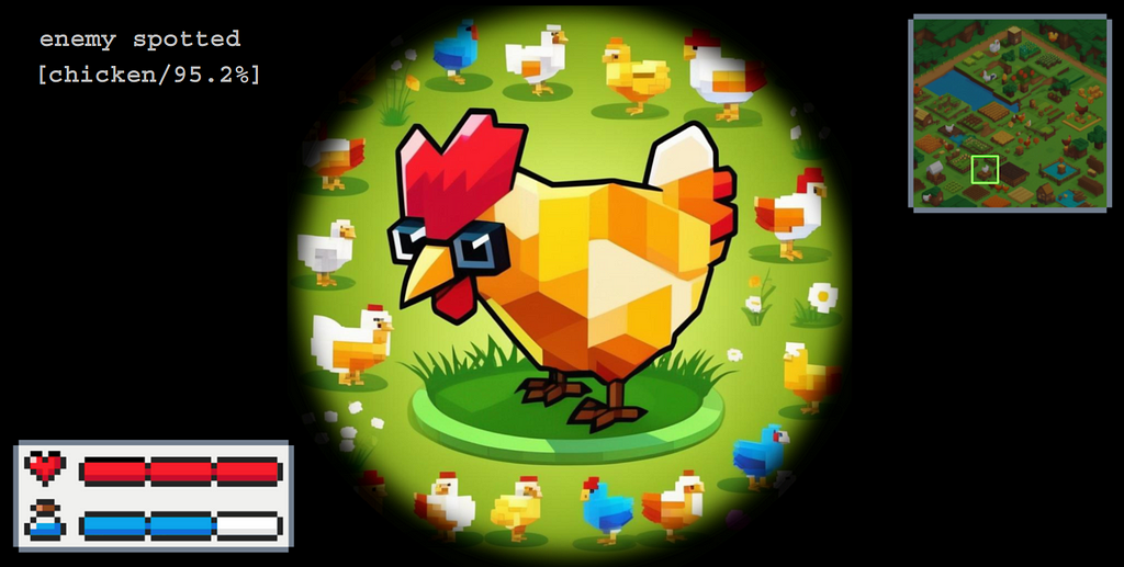

Recently, I came across one of the great cases of using Raspberry Pi and Python for creating a computer vision-based system for object detection. In short, one guy created a device that keeps the neighbor’s chickens away from his property. After following the Reddit thread, it became apparent that the problem is quite pervasive and not limited to certain bird species, if at all. The top rated comments include:
“I need one of these for the ducks my neighbor feeds and then they sh*t all over my lawn.” — Light_Beard
“I need this for cats in my yard at night.” — Buddha_
“Does it work on kids on Halloween? Asking for a friend.” — HardPawns
Well, one might argue that the problem is not that important and quite legitimately suggest simply asking the neighbors to sort out those hens. However, this is clearly not an engineer’s way to tackle this. Suppose you had already built an AI-assisted bird detection system equipped with a water blaster to chase unwelcome hens away from the yard. The caveat is that its operating version does not perform as well as expected, resulting in still noticeable water usage for sprinkling and lawn cleanup. Hence, chickens run and water bills remain lofty. How to address the challenge?
Here, we are about to tackle this real-world problem by designing a computational model to simulate the complete chicken-on-the-lawn cycle and later optimize its parameters so that we can reduce water consumption. To do so, we will employ different techniques, including those from automata theory and randomized algorithms.
In particular, this article focuses on modelling and simulation aspects so that you learn how to describe behavior of a real system and design a finite state machine reflecting its dynamics. Then, you will explore the path of implementing such systems in Python and discover ways to leverage computer vision-based models by optimizing its performance on object detection. This should be fun!
Disclaimer: This work is a part of the “Bird by Bird using Deep Learning” series and is devoted to modelling and simulation of real-life systems for computer vision applications using finite automata. All actors, states, events and outputs are the products of the FSM design process for educational purposes only. Any resemblance to actual persons, birds, or real events is purely coincidental.
Finite-state machine (FSM) or finite automaton is a mathematical model that can be used to represent and analyse dynamic behavior of a system by describing it through discrete states, transitions between those states, and a set of rules triggering these transitions.
The history of FSM traces back to the mid-20th century, marked by pivotal milestones in automata theory and the theory of computation. Early contributions by luminaries such as Alan Turing and John von Neumann laid the foundation, but it was in the 1950s and 1960s that FSM took a significant leap forward. Notably, Edward F. Moore and George H. Mealy independently introduced two primary types of FSMs, Moore and Mealy machines, respectively.
These FSM types differ in their approach: Moore machines determine next states based solely on the current state, while the Mealy ones associate outputs with the current state and input, offering enhanced adaptability. Originally used in digital circuits, FSMs, in particular Mealy machines, with their responsiveness to external input signals, have become widespread in the design of complex systems that accompany our daily lives.
FSMs are found in both hardware and software applications. Look around — almost all electronic and computing devices have some sort of finite automata — from vending machines to CPUs, from basic electronic devices to programmable logical controllers for smart home automation. They are also taken in software and game development and, of course, can be used to create adaptive AI-assisted systems for real-time object detection.
At its core, a deterministic finite automaton includes states, inputs, and a transition function. States represent distinct conditions of the system, while inputs trigger switches between states. The transition function defines rules of how the machine transitions between states. Mathematically, such state machine can be represented using a 5-tuple, denoted as M=(Q, Σ, δ, q₀, F), where:
This way, for any given state and specific input symbol, there is a unique next state determined by the transition function δ, which is typically represented by a state transition table or diagram, specifying transitions given a combination of the current state and inputs.
The design process of an FSM involves identifying the states (and inputs if applicable), defining the transition function, as well as specifying the initial and final states. The following methodology can be employed for translating complex systems into comprehensible models, aiding in the further analysis, design, and implementation phases. A 5-step FSM design process includes:
This iterative process allows to design a concise representation of the real system’s behavior, allowing for approximations and refinements along the process. For instance, after implementing an FSM (Step 4), you may want to further verify and update the specifications (Steps 2–3), same applies to moving from the experimentation (Step 5) back to the problem definition (Step 1), in order to create a working model that is sufficiently detailed and useful to solve a particular problem.
Let us take a simple case of the chicken-on-the-lawn scenario, where a bird can either be present on the lawn or not, as a function of external stimuli initiated by the engineer, who, in turn, can either rest or chase away unwelcome guests trespassing on his property. Thus, the controlling object (the engineer) is intended to compensate for the uncertainty of the independent actors (chickens) parameters. In the given example, the set of final states F includes only one state in which the system terminates, say at the end of the day when there are no chickens around. In this way:
Figure 1 provides a state transition diagram consisting of nodes (states) connected by edges (next-state transitions), with the labels above the arcs specifying input events triggering the transitions.
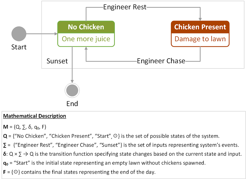
This representation captures the binary nature of the problem, in which a chicken can either be present or not on the lawn. The system responds to the events triggered by the engineer or the sunset. In the diagram, the initial and final states are indicated by circles. The transition function δ for this FSM can also be written in a tabular form, showing state transitions and control actions for the system, as shown in Table 1.
Table 1. State-transition table for the chicken-on-the-lawn FSM example

+========================+========================+========================+
| Current State          | Input Event            | Next State             |
+========================+========================+========================+
| q₀ ≡ ”No Bird”         | α₀ ≡ ”Engineer Rest”   | q₁                     |
+------------------------+------------------------+------------------------+
| q₁ ≡ ”Bird Present”    | α₁ ≡ ”Engineer Chase”  | q₀                     |
+------------------------+------------------------+------------------------+
| q₀                     | α₂ ≡ ”Sunset”          | ⊙                     |
+------------------------+------------------------+------------------------+
Thus, by completing five straightforward steps we designed a simple state machine. Now that everything has been explained, let’s finally create an FSM-based model representing our challenge with birds on the lawn.
As you have learnt in the previous section, finite automata can be used to model almost any process. Imagine you have some chickens hopping around in your backyard this afternoon. What are they doing? Just observe. They’re always moving, singing, or interacting. They’re often flying, probing, or eating. On some occasions, they’re displaying, or doing something that draws our attention, like those neighbor’s chickens messing up with the grass, but let’s set those particulars aside for now. Well, eventually, all the birds are s***ing (nothing personal, feathery ones). For the FSM design, we won’t get into the finer details, instead distilling essential components with logic for our simulation. Let the FSM take water adventures to the next level of play!
Concerning the chickens, here, we are going to describe the system to reflect our down-to-earth scenario in order to optimize parameters of the object detection system and reduce water costs for lawn cleaning. For the reference, take another look at the previous FSM example. This simple machine differs from the real-life system in some particular aspects. First, we want to actualize the controlling object to include an AI-based device aimed at detecting and repelling birds, this time by means of a high-pressure water sprinkler gun (so the engineer can “self-loop” into the rest state).
Second, we will need to update and/or extend the set of possible states, events, and transitions reflecting complexity of the updated system’s setup. For the latter, why don’t we consider additional bird categories that can be recognized by a computer vision model (e.g., turkeys) thus being potential independent actors for our FSM. Moreover, assuming that bird size varies across species, an irrigation control system would need a more intense water flow and/or pressure to successfully chase a bulky turkey off the lawn than it would for a chicken. Hereafter, for brevity’s sake, we will refer to the chicken-and-turkey-on-the-lawn problem as the CaT problem.
In order to model scenarios where the object detection system has to monitor, classify, and interact with objects trespassing on the property, we will define states, events, and transitions that represent the different aspects of this situation. Our goal is to capture the various states the object detection system and chickens can be in, as well as the events that trigger state transitions.
For the logic design scenarios, consider that at any given moment a bird can enter the yard, mess up with the lawn (or not), and leave the property either for its own or if it was successfully detected and chased away by the AI-based lawn security system. Now, let’s define some main components of the FSM simulation.
States represent possible conditions reflecting the CaT scenarios:
Transitions govern how the system switches between states based on inputs. For instance, the AI model may overlook a bird and miss the sprinkling process, thus, resulting in a number of consequences for the lawn. Here are some other scenarios and conditions we can anticipate:
This way, the FSM will dynamically progress from one state to another as the AI system interacts with the chickens hopping around. To make task easier and less error-prone, we create a combined state transition and conditions table:
Table 2. FSM inputs describing the events triggering state changes

+====+==================================+==================+================+
| ID | Input Description                | Defence System   | Enemy Tactics  |
|    |                                  | Operation Mode   | and Waypoints  |
+====+==================================+==================+================+
| X₁ | Bird is present on the lawn      |                  | Hopping        |
+----+----------------------------------+ Object detection +----------------+
| X₂ | Bird intrudes the lawn           |                  | Start hopping  |
+----+----------------------------------+------------------+----------------+
| X₃ | AI-powered detector spots a bird | Start sprinkling | Hopping (still)|
+----+----------------------------------+------------------+----------------+
| X₄ | Bird is hit successfully¹        |                  |                |
+----+----------------------------------+        -         | Intimidation   |
| X₅ | Target is susceptible²           |                  |                |
+----+----------------------------------+------------------+----------------+
| X₆ | Bird spoiled the lawn            |                  | Hopping merrily|
+----+----------------------------------+ Object detection +----------------+
| X₇ | Bird leaves the lawn             |                  | Retreat        |
+----+----------------------------------+------------------+----------------+
| X₈ | Simulation period ends (sunset)  |        -         | -              |
+----+----------------------------------+------------------+----------------+
ID - input identifier
¹ - aiming and sprinkling modules operated correctly
² - water flow rate is strong enough to chase the bird away
Now, after identifying states and events, we’ll write a combined state transition table with Boolean expressions for the next states. In table 3, we see how the inputs described in Table 2 steer the transitions between the simulation states.
Table 3. FSM state transition table with next-stage transition logic

+========================+========================+========================+
| Current State          | Transition Formula     | Next State             |
+========================+========================+========================+
| Start                  | TRUE                   | Spawn                  |
+------------------------+------------------------+------------------------+
|                        | X₁ ∨ X₂                | Intrusion              |
|                        |------------------------+------------------------+
| Spawn                  | ¬X₁ ∧ ¬X₂              | Empty lawn             |
+                        |------------------------+------------------------+
|                        | X₈                     | End                    |
+------------------------+------------------------+------------------------+
|                        | X₃                     | Target detected        |
| Intrusion              |------------------------+------------------------+
|                        | ¬X₃                    | Not detected           |
+------------------------+------------------------+------------------------+
|                        | X₃                     | Target detected        |
| Empty lawn             |------------------------+------------------------+
|                        | ¬X₃                    | Not detected           |
+------------------------+------------------------+------------------------+
| Target detected        | TRUE                   | Sprinkling             |
+------------------------+------------------------+------------------------+
|                        | X₁                     | Attacking              |
| Not detected           |------------------------+------------------------+
|                        | ¬X₁                    | Not attacked           |
+------------------------+------------------------+------------------------+
|                        | ¬X₁ ∨ ¬X₄ ∨ ¬X         | Miss                   |
| Sprinkling             |------------------------+------------------------+
|                        | X₁ ∧ X₄ ∧ X₅           | Hit                    |
+------------------------+------------------------+------------------------+
|                        | ¬X₁                    | Spawn                  |
| Miss                   |------------------------+------------------------+
|                        | X₁                     | Attacking              |
+------------------------+------------------------+------------------------+
| Hit                    | TRUE                   | Bird leaves            |
+------------------------+------------------------+------------------------+
|                        | ¬X₆                    | Not attacked           |
| Attacking              |------------------------+------------------------+
|                        | X₆                     | Bird attacked          |
+------------------------+------------------------+------------------------+
|                        | ¬X₇                    | Spawn                  |
| Not attacked           |------------------------+------------------------+
|                        | X₇                     | Bird leaves            |
+------------------------+------------------------+------------------------+
|                        | ¬X₇                    | Spawn                  |
| Bird attacked          |------------------------+------------------------+
|                        | X₇                     | Bird leaves            |
+------------------------+------------------------+------------------------+
| Bird leaves            | TRUE                   | Spawn                  |
+------------------------+------------------------+------------------------+
In most cases, a single input determines the next state. However, we have to consider a number of conditions simultaneously for switching from “Spawn” or “Sprinkling”. You could also notice that for some states, transitions don’t depend on the external information, like for “Start” or “Hit”. These states are either special (as “Start”) or trigger auxiliary actions. The latter don’t have a direct influence on the story we simulate (i.e. in that regard, they can be combined with the subsequent states) but are important for gathering simulation statistics.
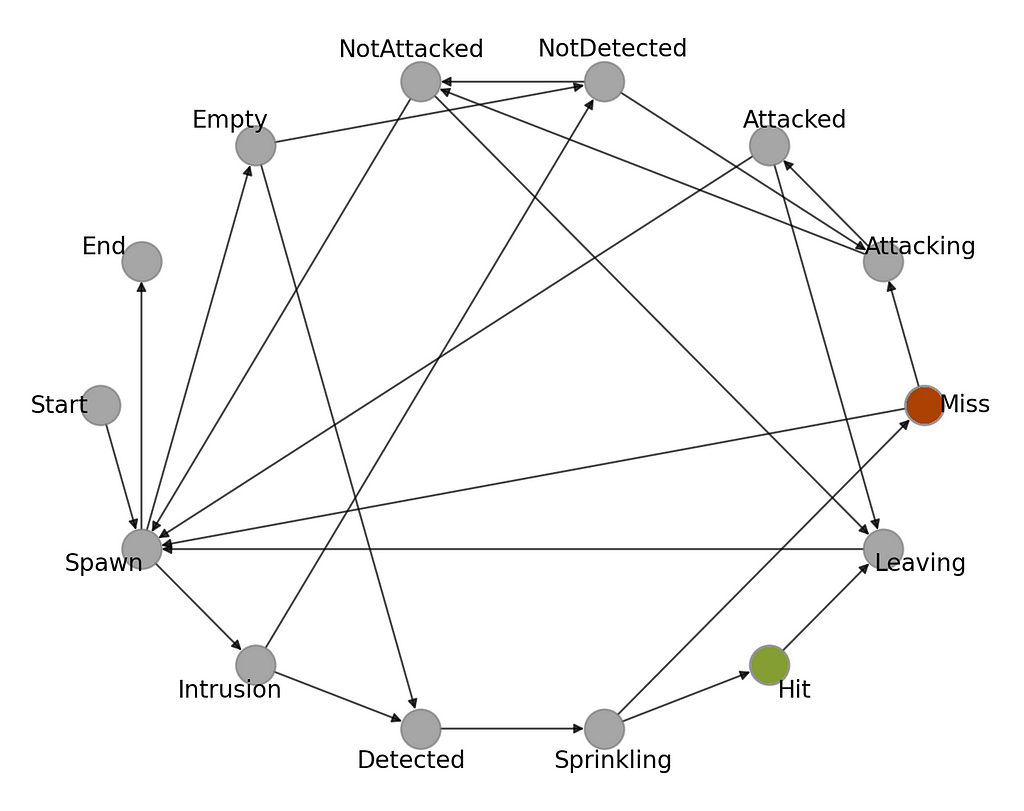
Finally, let’s look at its visual representation. Figure 3 presents the state transition graph corresponding to the CaT system going through during its lifetime. You can probably see the connection already. Moving forward with the following article, you will learn how to implement this FSM in Python and how to use it to optimize parameters of the AI-assisted bird detection system in order to reduce water cost.
In this article, we explored how to apply finite state machines in practice to build a model for addressing the CaT problem, allowing for high-level problem analysis and solution design.
We have described complex yard processes by applying the FSM formalism to individual actors and the interactions between them, thereby creating a holistic view of the internal dynamics of the real-world situation, in which we had to deal with neighborhood birds trespassing on the property.
This allowed us to create a simulation that reflects, among other things, the operation of the AI-assisted security system equipped with a water pressure controller for sprinkling and aimed at object detection and chasing away unwelcome guests spoiling the lawn.
In the upcoming series of articles, we will further investigate the topic of simulation of real-life scenarios using FSMs and its practical applications for addressing a non-analytic optimization problem of water cost reduction.
Specifically, the next article will feature a Python tutorial from which you will learn how to implement an FSM-driven simulation from scratch as well as how to employ it as a part of a stochastic optimization pipeline. Based on the simulation created, we then examine how to leverage it for improving the resource efficiency of our lawn security system by applying Monte-Carlo and eXplainable AI (XAI) techniques to optimize performance of a computer vision-based subsystem for bird detection.
Interested to keep it on? Stay updated on more materials at — https://github.com/slipnitskaya/caltech-birds-advanced-classification and https://medium.com/@slipnitskaya.
Finite Automata Simulation for Leveraging AI-Assisted Systems was originally published in Towards Data Science on Medium, where people are continuing the conversation by highlighting and responding to this story.
Originally appeared here:
Finite Automata Simulation for Leveraging AI-Assisted Systems
Go Here to Read this Fast! Finite Automata Simulation for Leveraging AI-Assisted Systems
Explore the architecture of Lag-Llama and learn to apply it in a forecasting project using Python
Originally appeared here:
Lag-Llama: Open-Source Foundation Model for Time Series Forecasting
Go Here to Read this Fast! Lag-Llama: Open-Source Foundation Model for Time Series Forecasting


This post will review different methods to run a dockerized Python environment from the command line (CLI). Am I recommending you run your Python environment from the CLI? Absolutely not!
There are better ways to set up a Python development environment, such as using VScode and the Dev Containers extension. We will use the “hard way” to set up a Python environment from the CLI for learning purposes. We will review different approaches to launching a container with the run command and see how to customize a built-in image using the Dockerfile.
To follow along with this tutorial, you will need the following:
Throughout this tutorial, we will use the official Python image — python:3.1o.
Let’s get started by pulling the official Python 3.10 image from Docker Hub. First, let’s log in to Docker Hub by using the docker logincommand:
docker login docker.io                                                                                                                                                                      ok
Authenticating with existing credentials...
Login Succeeded
Next, we will use the docker pull command from the terminal:
docker pull python:3.10 ok
If this is the first time you pull the image, you should expect the following output:
3.10: Pulling from library/python
66932e2b787d: Pull complete
4afa7e263db1: Pull complete
c812910e5e62: Pull complete
f4e4299bb649: Pull complete
5213cc2f9120: Pull complete
4a3b5b2f0e66: Pull complete
c214ceb1cabf: Pull complete
f5336038b15c: Pull complete
Digest: sha256:f94601bb6374b0b63835a70c9e5c3ba1b19bc009133900a9473229a406018e46
Status: Downloaded newer image for python:3.10
docker.io/library/python:3.10
You can review the image details with the use of the docker images command:
docker images                                                                                                                                                                          ok  11s
REPOSITORY   TAG       IMAGE ID       CREATED      SIZE
python       3.10      f7537c504c9a   7 days ago   1.01GB
Before running the container, let’s review the image metadata with the docker inspect command:
docker inspect python:3.10
This will return the below JSON output:
[
    {
        "Id": "sha256:f7537c504c9a91a22c9a255ee02048e7079cacdee583290e8238c605d17f9600",
        "RepoTags": [
            "python:3.10"
        ],
        "RepoDigests": [
            "python@sha256:f94601bb6374b0b63835a70c9e5c3ba1b19bc009133900a9473229a406018e46"
        ],
        "Parent": "",
        "Comment": "buildkit.dockerfile.v0",
        "Created": "2024-02-03T10:49:13Z",
        "Container": "",
        "ContainerConfig": {
            "Hostname": "",
            "Domainname": "",
            "User": "",
            "AttachStdin": false,
            "AttachStdout": false,
            "AttachStderr": false,
            "Tty": false,
            "OpenStdin": false,
            "StdinOnce": false,
            "Env": null,
            "Cmd": null,
            "Image": "",
            "Volumes": null,
            "WorkingDir": "",
            "Entrypoint": null,
            "OnBuild": null,
            "Labels": null
        },
        "DockerVersion": "",
        "Author": "",
        "Config": {
            "Hostname": "",
            "Domainname": "",
            "User": "",
            "AttachStdin": false,
            "AttachStdout": false,
            "AttachStderr": false,
            "Tty": false,
            "OpenStdin": false,
            "StdinOnce": false,
            "Env": [
                "PATH=/usr/local/bin:/usr/local/sbin:/usr/local/bin:/usr/sbin:/usr/bin:/sbin:/bin",
                "LANG=C.UTF-8",
                "GPG_KEY=A035C8C19219BA821ECEA86B64E628F8D684696D",
                "PYTHON_VERSION=3.10.13",
                "PYTHON_PIP_VERSION=23.0.1",
                "PYTHON_SETUPTOOLS_VERSION=65.5.1",
                "PYTHON_GET_PIP_URL=https://github.com/pypa/get-pip/raw/dbf0c85f76fb6e1ab42aa672ffca6f0a675d9ee4/public/get-pip.py",
                "PYTHON_GET_PIP_SHA256=dfe9fd5c28dc98b5ac17979a953ea550cec37ae1b47a5116007395bfacff2ab9"
            ],
            "Cmd": [
                "python3"
            ],
            "ArgsEscaped": true,
            "Image": "",
            "Volumes": null,
            "WorkingDir": "",
            "Entrypoint": null,
            "OnBuild": null,
            "Labels": null
        },
        "Architecture": "arm64",
        "Variant": "v8",
        "Os": "linux",
        "Size": 1005570383,
        "VirtualSize": 1005570383,
        "GraphDriver": {
            "Data": {
                "LowerDir": "/var/lib/docker/overlay2/d2fd76e7396796018a959209b51fe8311a188c8eae8e339e9e556de0889ca0bd/diff:/var/lib/docker/overlay2/bbedb25c5aa6ec3f2fc632e62a53989a329b907143fac165f899209293627a69/diff:/var/lib/docker/overlay2/ed6a4bf49214e6b496b7716443b8de380481cd9416bc4a378f29183c9129786f/diff:/var/lib/docker/overlay2/ac9543f44a835c203fb0b0b28958d94df72d206c9060c9d83307b39f50355102/diff:/var/lib/docker/overlay2/94a9f92c36ea6251feda52be8e76ec4da4a9c66b744a29472e1ccfdf34a6f69d/diff:/var/lib/docker/overlay2/6ee22c274256834a64008022856d365d91373bb490ae9f2f1723cb524b246a29/diff:/var/lib/docker/overlay2/2fa272376e0ce68f4f34f18e5ecb1ddd58a32fb20a82e5a417514047f8e684a3/diff",
                "MergedDir": "/var/lib/docker/overlay2/f2d64d1affbe99afb05251435f7705cb97e2efa4f8febb494b4cbaa21e7f742a/merged",
                "UpperDir": "/var/lib/docker/overlay2/f2d64d1affbe99afb05251435f7705cb97e2efa4f8febb494b4cbaa21e7f742a/diff",
                "WorkDir": "/var/lib/docker/overlay2/f2d64d1affbe99afb05251435f7705cb97e2efa4f8febb494b4cbaa21e7f742a/work"
            },
            "Name": "overlay2"
        },
        "RootFS": {
            "Type": "layers",
            "Layers": [
                "sha256:9f8c60461a42fd9f275c56f4ec8fea8a8ea2d938493e316e830994a3814cf0aa",
                "sha256:927a28cdbf6c1705342b2cba0069457313815058dcebe1996e46cade38a09370",
                "sha256:e85139d96aee18e99fc964d02546be48cc6a4d4dfd9f465a91f172b7c535e55f",
                "sha256:f3168ba6a8d2ec30e12002ad5b7b497cf7409f3e19cc8d8f447f6cf4231a2482",
                "sha256:acbc6c8127209b09fa336e354037fdc630d3594e15174f2bc1bdbf31d5591376",
                "sha256:06c4da96c7dd2fbbbb541e000bd0ea4cfbf7c80b24f098a9d67f677ef5e6c63e",
                "sha256:1cdf208dc10679cf5db6d4f0e17ff6d5bfe754b4195ddd3b153b6d1ff51ce909",
                "sha256:5d6f554f67c7da9d34763916bac632a450902c6e6fdbf9244f888f110fd37740"
            ]
        },
        "Metadata": {
            "LastTagTime": "0001-01-01T00:00:00Z"
        }
    }
]
The ispect command provides a lot of useful information about the image, such as the layers information, the image size, the hardware architecture, etc. As we want to run the image, the most interesting detail is the CMD setting. The CMDcommand in the Dockerfile defines what command to execute during the container launch time. We can parse from the above output the CMD information with the jq package:
docker inspect python:3.10 | jq '.[] | .Config | .Cmd'                                                                                                                                      ok
[
  "python3"
]
As you can see, the image is set to execute the python3 command during the container run time. Let’s now launch the container using the run command:
docker run python:3.10
And… nothing happens. The reason for that, in short, is that we need to give Docker access to the terminal. We will use the interactive and TTY arguments to run the image in an interactive mode:
docker run --interactive --tty python:3.10
This will attach the terminal to the container and open Python inside the container:
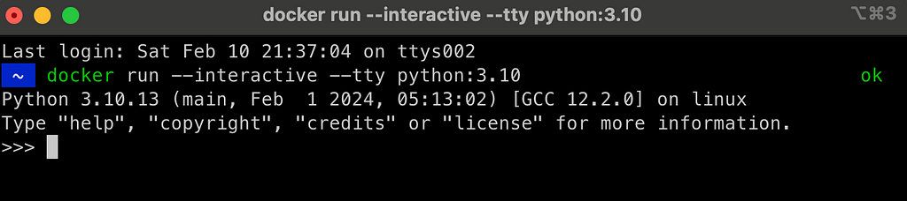
While we were able to launch Python inside a container, it is not as useful:
For example, if we will try to load pandas, we will get the following error:
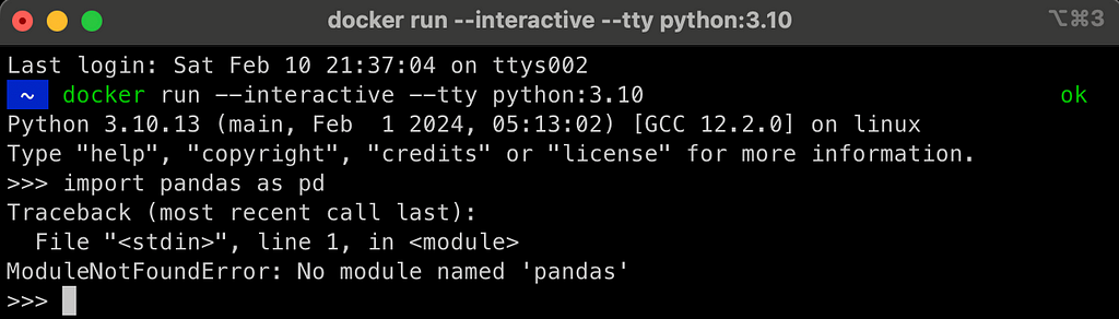
In the following sections, we will address those issues by creating a Dockerfile and customizing the base image functionality. This includes adding the following features:
To customize the Python environment and make the above changes, we will create a Dockerfile with the following functionality:
To set up a Python virtual environment, we will use the following two helper files:
requirements.txt
wheel==0.40.0
pandas==2.0.3
This file defines the list of Python libraries to install in the virtual environment. For example, in this case, we will install the Pandas library, version 2.0.3. Generally, I also install the wheels library, which handles C dependencies.
The next helper file is the below bash script, which sets the virtual environment and installs the required libraries from the requirements.txt file.
set_python_env.sh
#!/usr/bin/env bash

PYTHON_ENV=$1

python3 -m venv /opt/$PYTHON_ENV
        && export PATH=/opt/$PYTHON_ENV/bin:$PATH
        && echo "source /opt/$PYTHON_ENV/bin/activate" >> ~/.bashrc

source /opt/$PYTHON_ENV/bin/activate

pip3 install -r ./requirements/requirements.txt
Note: We use a variable (marked as $1) to define the environment name, which will be assigned to the PYTHON_ENV variable. Using variables during the build is a good practice, as it enables us to modify some of the image characteristics without modifying the code. We will assign the variable via the Dockerfile.
Let’s explain the following concatenate code from the above bash script that sets the virtual environment:
python3 -m venv /opt/$PYTHON_ENV
    && export PATH=/opt/$PYTHON_ENV/bin:$PATH
    && echo "source /opt/$PYTHON_ENV/bin/activate" >> ~/.bashrc
The above three lines of code include three concatenate expressions:
Once the environment is set, we use the source command to activate the environment, and the pip3 command to install the libraries inside the environment.
After we review the helper files, let’s see how they are incorporated inside the below Dockerfile.
Dockerfile
FROM python:3.10

ARG PYTHON_ENV=my_env
ENV PYTHON_ENV=$PYTHON_ENV

RUN mkdir requirements

COPY requirements.txt set_python_env.sh /requirements/

RUN bash ./requirements/set_python_env.sh $PYTHON_ENV

RUN apt-get update &&
    apt-get install -y
    vim
    && apt update


CMD ["/bin/sh", "-c", "bash"]
As you can see, we are using the same image — python:3.10as our base image.
Next, we set an argument named PYTHON_ENV with the ARG command to define the virtual environment name. We setmy_env as the default value, which can be modified during the build time using the arg argument. We use the PYTHON_ENV argument to set an environment variable as well.
Before setting the virtual environment, we will create inside the image a new library under the root folder named requirements and use the COPY command to copy the above helper files — requirements.txt and set_my_python.sh to the requirements folder.
Next, we call the bash script — set_my_python.sh , which sets the virtual environment and installs the required libraries. As mentioned above, we use the PYTHON_ENV variable as an argument with the set_my_python.sh file to set the virtual environment name dynamically.
We use the apt command to install vim — a CLI editor. This will enable us to edit code on via the container CLI.
Last but not least, use the CMD command to launch a shell terminal using bash:
CMD ["/bin/sh", "-c", "bash"]
At this point, we have the below files in the local folder:
.
├── Dockerfile
├── requirements.txt
└── set_python_env.sh
Let’s now go ahead and build the image with the docker build command:
docker build .-f Dockerfile -t my_python_env:3.10
[+] Building 47.3s (10/10) FINISHED
 => [internal] load build definition from Dockerfile                                                 0.2s
 => => transferring dockerfile: 389B                                                                 0.0s
 => [internal] load .dockerignore                                                                    0.2s
 => => transferring context: 2B                                                                      0.0s
 => [internal] load metadata for docker.io/library/python:3.10                                       0.0s
 => [1/5] FROM docker.io/library/python:3.10                                                         1.3s
 => [internal] load build context                                                                    0.4s
 => => transferring context: 460B                                                                    0.0s
 => [2/5] RUN mkdir requirements                                                                     0.5s
 => [3/5] COPY requirements.txt set_python_env.sh /requirements/                                     0.2s
 => [4/5] RUN bash ./requirements/set_python_env.sh my_env                                          26.8s
 => [5/5] RUN apt-get update &&     apt-get install -y     vim     && apt update                    17.4s
 => exporting to image                                                                               0.7s
 => => exporting layers                                                                              0.6s
 => => writing image sha256:391879baceea6154c191692d4bcb9ec9690de6dc4d5edd5b2ed13f6c579dd05c         0.0s
 => => naming to docker.io/library/my_python_env:3.10
Let’s run again the docker images command to review the current images:
docker images
REPOSITORY      TAG       IMAGE ID       CREATED         SIZE
my_python_env   3.10      391879baceea   7 minutes ago   1.23GB
python          3.10      f7537c504c9a   8 days ago      1.01GB
As you can note, adding the virtual environment and installing the packages added about 250 Mb to the image size.
After we built the image, let’s launch the image with the docker run command and check if the above properties are defined as expected:
docker run --interactive --tty my_python_env:3.10
This launches the image in interactive mode, and opens a bash terminal as expected:
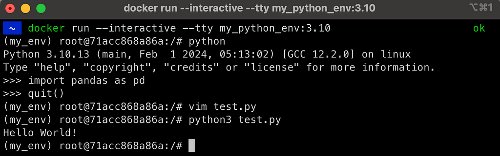
As you can notice in the above screenshot, it launched the container inside the bash terminal, and the virtual environment is set as expected as my_env. The pandas library was installed and can be loaded, and we can now edit files from the terminal.
One issue to take care of is that the container is still ephemeral. Therefore, any code we create inside the image is not exportable and will be lost after we stop the container from running.
A simple solution is to mount a volume with the volume argument. For simplicity, we will go ahead and mount the local folder, where we keep the Dockerfile and the helper files, to a new folder inside the container named my_scripts:
docker run -v .:/my_scripts --interactive --tty my_python_env:3.10
And here is the output:
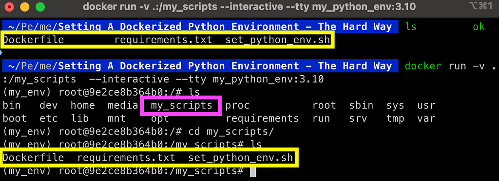
Once the folder is mounted, any file that is created, modified, or deleted from the mounted folder inside the container will be reflected to the local folder. This enables you to maintain your code when stopping the container.
In this tutorial, we reviewed how to set a dockerized Python environment using the command line. While this is neither a practical nor recommended approach to develop with Python, it is a great learning experience of Docker core commands and basic functionalities. We show how we can easily take a built-in image and customize it according to our needs. Last but not least, we saw how to mount a local folder to the container with the volume argument to transfer the container from an ephemeral mode to a persistent mode.
Setting A Dockerized Python Environment — The Hard Way was originally published in Towards Data Science on Medium, where people are continuing the conversation by highlighting and responding to this story.
Originally appeared here:
Setting A Dockerized Python Environment — The Hard Way
Go Here to Read this Fast! Setting A Dockerized Python Environment — The Hard Way

As human beings, we can read and understand texts (at least some of them). Computers in opposite “think in numbers”, so they can’t automatically grasp the meaning of words and sentences. If we want computers to understand the natural language, we need to convert this information into the format that computers can work with — vectors of numbers.
People learned how to convert texts into machine-understandable format many years ago (one of the first versions was ASCII). Such an approach helps render and transfer texts but doesn’t encode the meaning of the words. At that time, the standard search technique was a keyword search when you were just looking for all the documents that contained specific words or N-grams.
Then, after decades, embeddings have emerged. We can calculate embeddings for words, sentences, and even images. Embeddings are also vectors of numbers, but they can capture the meaning. So, you can use them to do a semantic search and even work with documents in different languages.
In this article, I would like to dive deeper into the embedding topic and discuss all the details:
Let’s move on and learn about the evolution of embeddings.
We will start our journey with a brief tour into the history of text representations.
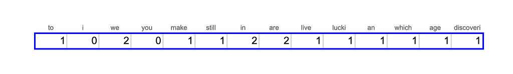
The most basic approach to converting texts into vectors is a bag of words. Let’s look at one of the famous quotes of Richard P. Feynman“We are lucky to live in an age in which we are still making discoveries”. We will use it to illustrate a bag of words approach.
The first step to get a bag of words vector is to split the text into words (tokens) and then reduce words to their base forms. For example, “running” will transform into “run”. This process is called stemming. We can use the NLTK Python package for it.
from nltk.stem import SnowballStemmer
from nltk.tokenize import word_tokenize

text = 'We are lucky to live in an age in which we are still making discoveries'

# tokenization - splitting text into words
words = word_tokenize(text)
print(words)
# ['We', 'are', 'lucky', 'to', 'live', 'in', 'an', 'age', 'in', 'which',
#  'we', 'are', 'still', 'making', 'discoveries']

stemmer = SnowballStemmer(language = "english")
stemmed_words = list(map(lambda x: stemmer.stem(x), words))
print(stemmed_words)
# ['we', 'are', 'lucki', 'to', 'live', 'in', 'an', 'age', 'in', 'which',
#  'we', 'are', 'still', 'make', 'discoveri']
Now, we have a list of base forms of all our words. The next step is to calculate their frequencies to create a vector.
import collections
bag_of_words = collections.Counter(stemmed_words)
print(bag_of_words)
# {'we': 2, 'are': 2, 'in': 2, 'lucki': 1, 'to': 1, 'live': 1,
# 'an': 1, 'age': 1, 'which': 1, 'still': 1, 'make': 1, 'discoveri': 1}
Actually, if we wanted to convert our text into a vector, we would have to take into account not only the words we have in the text but the whole vocabulary. Let’s assume we also have “i”, “you” and ”study” in our vocabulary and let’s create a vector from Feynman’s quote.
This approach is quite basic, and it doesn’t take into account the semantic meaning of the words, so the sentences “the girl is studying data science” and “the young woman is learning AI and ML” won’t be close to each other.
A slightly improved version of the bag of the words approach is TF-IDF (Term Frequency — Inverse Document Frequency). It’s the multiplication of two metrics.


So, in the end, we will get vectors where common words (like “I” or “you”) will have low weights, while rare words that occur in the document multiple times will have higher weights. This strategy will give a bit better results, but it still can’t capture semantic meaning.
The other challenge with this approach is that it produces pretty sparse vectors. The length of the vectors is equal to the corpus size. There are about 470K unique words in English (source), so we will have huge vectors. Since the sentence won’t have more than 50 unique words, 99.99% of the values in vectors will be 0, not encoding any info. Looking at this, scientists started to think about dense vector representation.
One of the most famous approaches to dense representation is word2vec, proposed by Google in 2013 in the paper “Efficient Estimation of Word Representations in Vector Space” by Mikolov et al.
There are two different word2vec approaches mentioned in the paper: Continuous Bag of Words (when we predict the word based on the surrounding words) and Skip-gram (the opposite task — when we predict context based on the word).
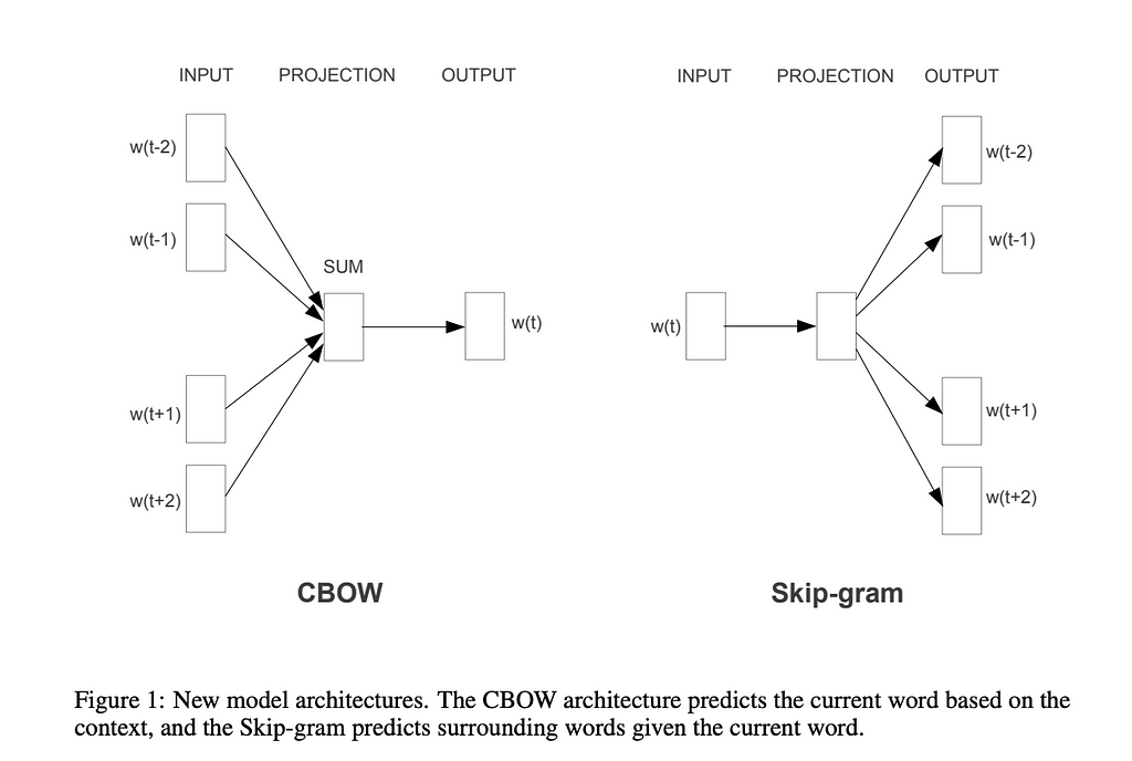
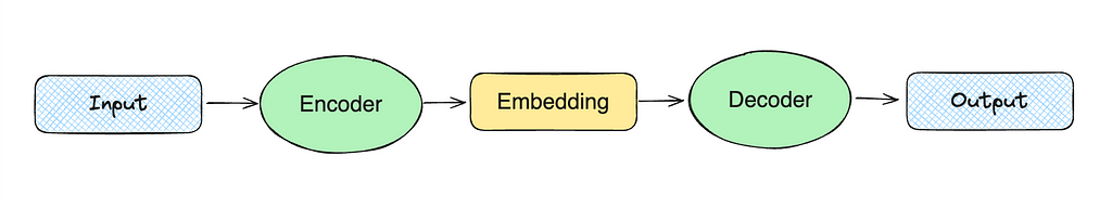
The high-level idea of dense vector representation is to train two models: encoder and decoder. For example, in the case of skip-gram, we might pass the word “christmas” to the encoder. Then, the encoder will produce a vector that we pass to the decoder expecting to get the words “merry”, “to”, and “you”.
This model started to take into account the meaning of the words since it’s trained on the context of the words. However, it ignores morphology (information we can get from the word parts, for example, that “-less” means the lack of something). This drawback was addressed later by looking at subword skip-grams in GloVe.
Also, word2vec was capable of working only with words, but we would like to encode whole sentences. So, let’s move on to the next evolutional step with transformers.
The next evolution was related to the transformers approach introduced in the “Attention Is All You Need” paper by Vaswani et al. Transformers were able to produce information-reach dense vectors and become the dominant technology for modern language models.
I won’t cover the details of the transformers’ architecture since it’s not so relevant to our topic and would take a lot of time. If you’re interested in learning more, there are a lot of materials about transformers, for example, “Transformers, Explained” or “The Illustrated Transformer”.
Transformers allow you to use the same “core” model and fine-tune it for different use cases without retraining the core model (which takes a lot of time and is quite costly). It led to the rise of pre-trained models. One of the first popular models was BERT (Bidirectional Encoder Representations from Transformers) by Google AI.
Internally, BERT still operates on a token level similar to word2vec, but we still want to get sentence embeddings. So, the naive approach could be to take an average of all tokens’ vectors. Unfortunately, this approach doesn’t show good performance.
This problem was solved in 2019 when Sentence-BERT was released. It outperformed all previous approaches to semantic textual similarity tasks and allowed the calculation of sentence embeddings.
It’s a huge topic so we won’t be able to cover it all in this article. So, if you’re really interested, you can learn more about the sentence embeddings in this article.
We’ve briefly covered the evolution of embeddings and got a high-level understanding of the theory. Now, it’s time to move on to practice and lear how to calculate embeddings using OpenAI tools.
In this article, we will be using OpenAI embeddings. We will try a new model text-embedding-3-small that was released just recently. The new model shows better performance compared to text-embedding-ada-002:
OpenAI also released a new larger model text-embedding-3-large. Now, it’s their best performing embedding model.
As a data source, we will be working with a small sample of Stack Exchange Data Dump — an anonymised dump of all user-contributed content on the Stack Exchange network. I’ve selected a bunch of topics that look interesting to me and sample 100 questions from each of them. Topics range from Generative AI to coffee or bicycles so that we will see quite a wide variety of topics.
First, we need to calculate embeddings for all our Stack Exchange questions. It’s worth doing it once and storing results locally (in a file or vector storage). We can generate embeddings using the OpenAI Python package.
from openai import OpenAI
client = OpenAI()

def get_embedding(text, model="text-embedding-3-small"):
   text = text.replace("n", " ")
   return client.embeddings.create(input = [text], model=model)
       .data[0].embedding

get_embedding("We are lucky to live in an age in which we are still making discoveries.")
As a result, we got a 1536-dimension vector of float numbers. We can now repeat it for all our data and start analysing the values.
The primary question you might have is how close the sentences are to each other by meaning. To uncover answers, let’s discuss the concept of distance between vectors.
Embeddings are actually vectors. So, if we want to understand how close two sentences are to each other, we can calculate the distance between vectors. A smaller distance would be equivalent to a closer semantic meaning.
Different metrics can be used to measure the distance between two vectors:
Let’s discuss them. As a simple example, we will be using two 2D vectors.
vector1 = [1, 4]
vector2 = [2, 2]
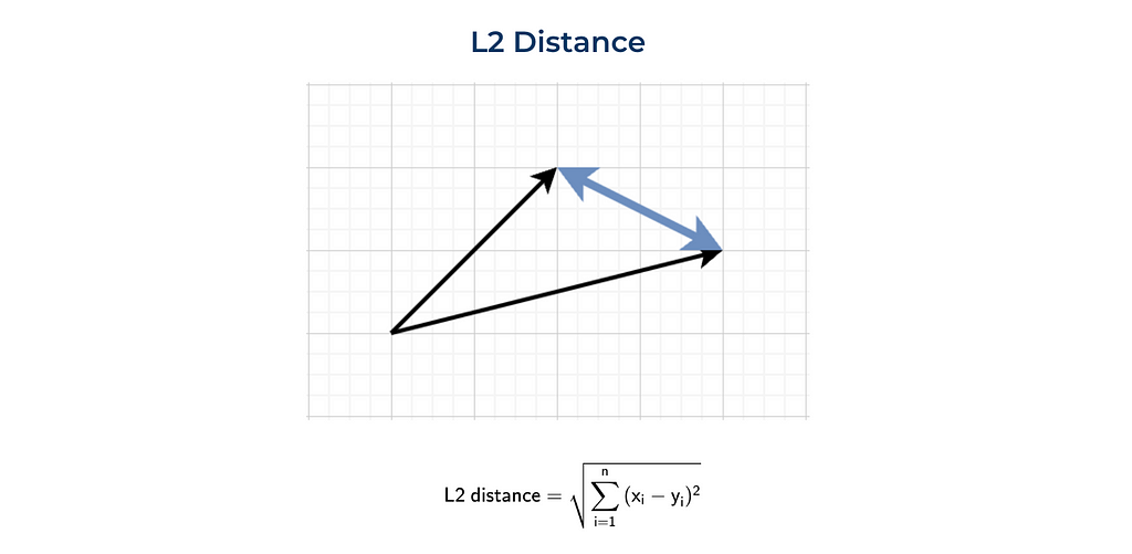
The most standard way to define distance between two points (or vectors) is Euclidean distance or L2 norm. This metric is the most commonly used in day-to-day life, for example, when we are talking about the distance between 2 towns.
Here’s a visual representation and formula for L2 distance.
We can calculate this metric using vanilla Python or leveraging the numpy function.
import numpy as np

sum(list(map(lambda x, y: (x - y) ** 2, vector1, vector2))) ** 0.5
# 2.2361

np.linalg.norm((np.array(vector1) - np.array(vector2)), ord = 2)
# 2.2361
The other commonly used distance is the L1 norm or Manhattan distance. This distance was called after the island of Manhattan (New York). This island has a grid layout of streets, and the shortest routes between two points in Manhattan will be L1 distance since you need to follow the grid.
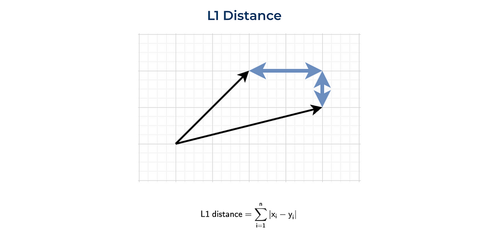
We can also implement it from scratch or use the numpy function.
sum(list(map(lambda x, y: abs(x - y), vector1, vector2)))
# 3

np.linalg.norm((np.array(vector1) - np.array(vector2)), ord = 1)
# 3.0
Another way to look at the distance between vectors is to calculate a dot or scalar product. Here’s a formula and we can easily implement it.

sum(list(map(lambda x, y: x*y, vector1, vector2)))
# 11

np.dot(vector1, vector2)
# 11
This metric is a bit tricky to interpret. On the one hand, it shows you whether vectors are pointing in one direction. On the other hand, the results highly depend on the magnitudes of the vectors. For example, let’s calculate the dot products between two pairs of vectors:
In both cases, vectors are collinear, but the dot product is ten times bigger in the second case: 2 vs 20.
Quite often, cosine similarity is used. Cosine similarity is a dot product normalised by vectors’ magnitudes (or normes).
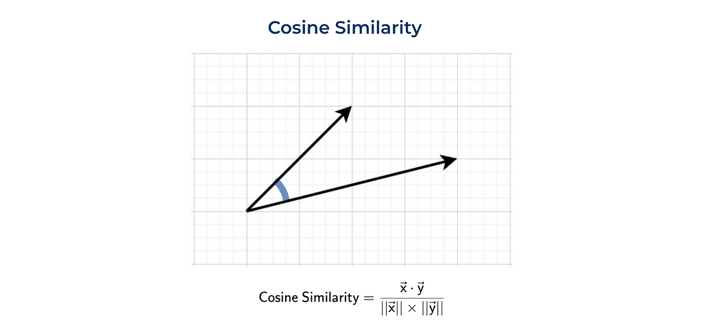
We can either calculate everything ourselves (as previously) or use the function from sklearn.
dot_product = sum(list(map(lambda x, y: x*y, vector1, vector2)))
norm_vector1 = sum(list(map(lambda x: x ** 2, vector1))) ** 0.5
norm_vector2 = sum(list(map(lambda x: x ** 2, vector2))) ** 0.5

dot_product/norm_vector1/norm_vector2

# 0.8575

from sklearn.metrics.pairwise import cosine_similarity

cosine_similarity(
  np.array(vector1).reshape(1, -1),
  np.array(vector2).reshape(1, -1))[0][0]

# 0.8575
The function cosine_similarity expects 2D arrays. That’s why we need to reshape the numpy arrays.
Let’s talk a bit about the physical meaning of this metric. Cosine similarity is equal to the cosine between two vectors. The closer the vectors are, the higher the metric value.
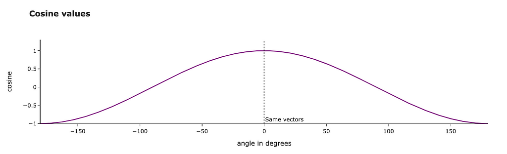
We can even calculate the exact angle between our vectors in degrees. We get results around 30 degrees, and it looks pretty reasonable.
import math
math.degrees(math.acos(0.8575))

# 30.96
We’ve discussed different ways to calculate the distance between two vectors, and you might start thinking about which one to use.
You can use any distance to compare the embeddings you have. For example, I calculated the average distances between the different clusters. Both L2 distance and cosine similarity show us similar pictures:
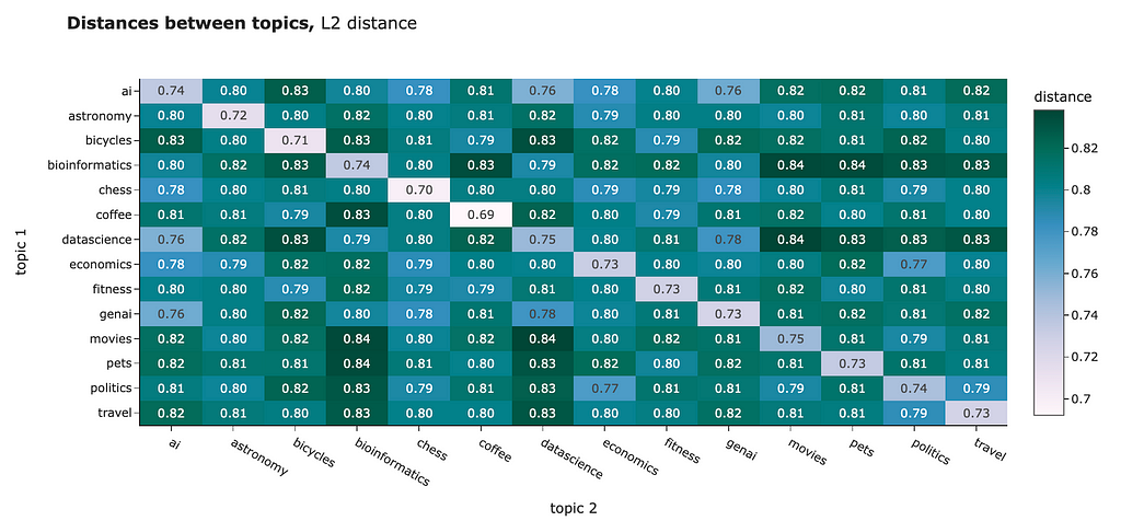
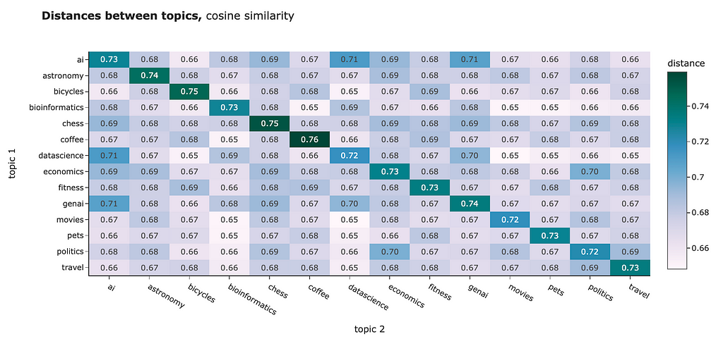
However, for NLP tasks, the best practice is usually to use cosine similarity. Some reasons behind it:
OpenAI embeddings are already normed, so dot product and cosine similarity are equal in this case.
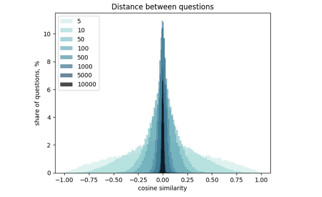
You might spot in the results above that the difference between inter- and intra-cluster distances is not so big. The root cause is the high dimensionality of our vectors. This effect is called “the curse of dimensionality”: the higher the dimension, the narrower the distribution of distances between vectors. You can learn more details about it in this article.
I would like to briefly show you how it works so that you get some intuition. I calculated a distribution of OpenAI embedding values and generated sets of 300 vectors with different dimensionalities. Then, I calculated the distances between all the vectors and draw a histogram. You can easily see that the increase in vector dimensionality makes the distribution narrower.
We’ve learned how to measure the similarities between the embeddings. With that we’ve finished with a theoretical part and moving to more practical part (visualisations and practical applications). Let’s start with visualisations since it’s always better to see your data first.
The best way to understand the data is to visualise it. Unfortunately, embeddings have 1536 dimensions, so it’s pretty challenging to look at the data. However, there’s a way: we could use dimensionality reduction techniques to project vectors in two-dimensional space.
The most basic dimensionality reduction technique is PCA (Principal Component Analysis). Let’s try to use it.
First, we need to convert our embeddings into a 2D numpy array to pass it to sklearn.
import numpy as np
embeddings_array = np.array(df.embedding.values.tolist())
print(embeddings_array.shape)
# (1400, 1536)
Then, we need to initialise a PCA model with n_components = 2 (because we want to create a 2D visualisation), train the model on the whole data and predict new values.
from sklearn.decomposition import PCA

pca_model = PCA(n_components = 2)
pca_model.fit(embeddings_array)

pca_embeddings_values = pca_model.transform(embeddings_array)
print(pca_embeddings_values.shape)
# (1400, 2)
As a result, we got a matrix with just two features for each question, so we could easily visualise it on a scatter plot.
fig = px.scatter(
    x = pca_embeddings_values[:,0],
    y = pca_embeddings_values[:,1],
    color = df.topic.values,
    hover_name = df.full_text.values,
    title = 'PCA embeddings', width = 800, height = 600,
    color_discrete_sequence = plotly.colors.qualitative.Alphabet_r
)

fig.update_layout(
    xaxis_title = 'first component',
    yaxis_title = 'second component')
fig.show()
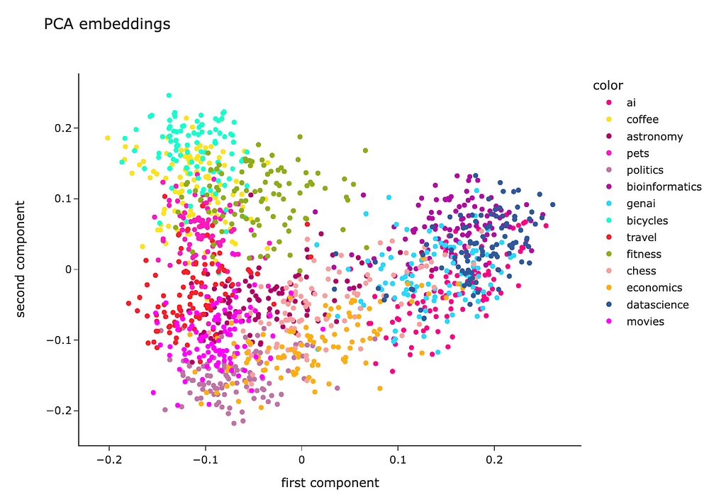
We can see that questions from each topic are pretty close to each other, which is good. However, all the clusters are mixed, so there’s room for improvement.
PCA is a linear algorithm, while most of the relations are non-linear in real life. So, we may not be able to separate the clusters because of non-linearity. Let’s try to use a non-linear algorithm t-SNE and see whether it will be able to show better results.
The code is almost identical. I just used the t-SNE model instead of PCA.
from sklearn.manifold import TSNE
tsne_model = TSNE(n_components=2, random_state=42)
tsne_embeddings_values = tsne_model.fit_transform(embeddings_array)

fig = px.scatter(
    x = tsne_embeddings_values[:,0],
    y = tsne_embeddings_values[:,1],
    color = df.topic.values,
    hover_name = df.full_text.values,
    title = 't-SNE embeddings', width = 800, height = 600,
    color_discrete_sequence = plotly.colors.qualitative.Alphabet_r
)

fig.update_layout(
    xaxis_title = 'first component',
    yaxis_title = 'second component')
fig.show()
The t-SNE result looks way better. Most of the clusters are separated except “genai”, “datascience” and “ai”. However, it’s pretty expected — I doubt I could separate these topics myself.
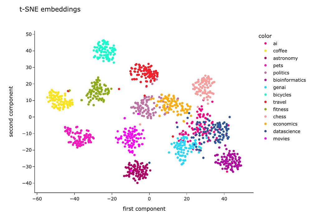
Looking at this visualisation, we see that embeddings are pretty good at encoding semantic meaning.
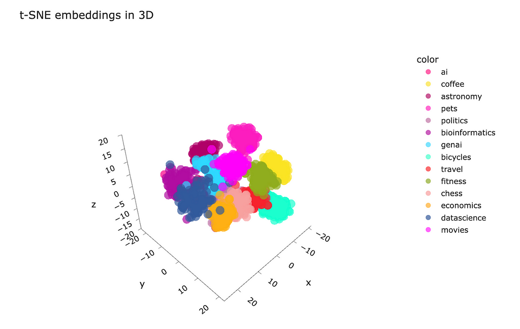
Also, you can make a projection to three-dimensional space and visualise it. I’m not sure whether it would be practical, but it can be insightful and engaging to play with the data in 3D.
tsne_model_3d = TSNE(n_components=3, random_state=42)
tsne_3d_embeddings_values = tsne_model_3d.fit_transform(embeddings_array)

fig = px.scatter_3d(
    x = tsne_3d_embeddings_values[:,0],
    y = tsne_3d_embeddings_values[:,1],
    z = tsne_3d_embeddings_values[:,2],
    color = df.topic.values,
    hover_name = df.full_text.values,
    title = 't-SNE embeddings', width = 800, height = 600,
    color_discrete_sequence = plotly.colors.qualitative.Alphabet_r,
    opacity = 0.7
)
fig.update_layout(xaxis_title = 'first component', yaxis_title = 'second component')
fig.show()
The way to understand the embeddings is to visualise a couple of them as bar codes and see the correlations. I picked three examples of embeddings: two are closest to each other, and the other is the farthest example in our dataset.
embedding1 = df.loc[1].embedding
embedding2 = df.loc[616].embedding
embedding3 = df.loc[749].embedding
import seaborn as sns
import matplotlib.pyplot as plt
embed_len_thr = 1536

sns.heatmap(np.array(embedding1[:embed_len_thr]).reshape(-1, embed_len_thr),
    cmap = "Greys", center = 0, square = False,
    xticklabels = False, cbar = False)
plt.gcf().set_size_inches(15,1)
plt.yticks([0.5], labels = ['AI'])
plt.show()

sns.heatmap(np.array(embedding3[:embed_len_thr]).reshape(-1, embed_len_thr),
    cmap = "Greys", center = 0, square = False,
    xticklabels = False, cbar = False)
plt.gcf().set_size_inches(15,1)
plt.yticks([0.5], labels = ['AI'])
plt.show()

sns.heatmap(np.array(embedding2[:embed_len_thr]).reshape(-1, embed_len_thr),
    cmap = "Greys", center = 0, square = False,
    xticklabels = False, cbar = False)
plt.gcf().set_size_inches(15,1)
plt.yticks([0.5], labels = ['Bioinformatics'])
plt.show()
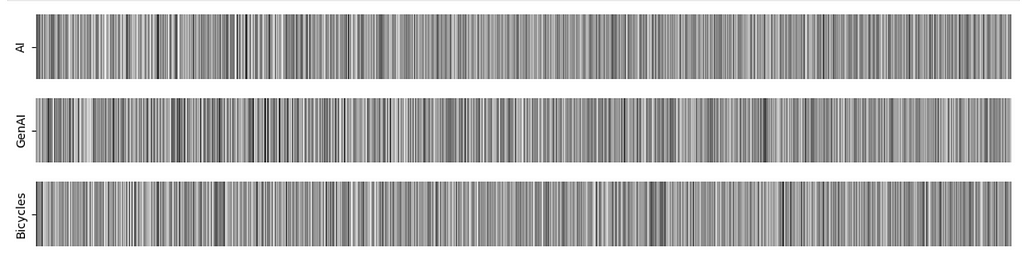
It’s not easy to see whether vectors are close to each other in our case because of high dimensionality. However, I still like this visualisation. It might be helpful in some cases, so I am sharing this idea with you.
We’ve learned how to visualise embeddings and have no doubts left about their ability to grasp the meaning of the text. Now, it’s time to move on to the most interesting and fascinating part and discuss how you can leverage embeddings in practice.
Of course, embeddings’ primary goal is not to encode texts as vectors of numbers or visualise them just for the sake of it. We can benefit a lot from our ability to capture the texts’ meanings. Let’s go through a bunch of more practical examples.
Let’s start with clustering. Clustering is an unsupervised learning technique that allows you to split your data into groups without any initial labels. Clustering can help you understand the internal structural patterns in your data.
We will use one of the most basic clustering algorithms — K-means. For the K-means algorithm, we need to specify the number of clusters. We can define the optimal number of clusters using silhouette scores.
Let’s try k (number of clusters) between 2 and 50. For each k, we will train a model and calculate silhouette scores. The higher silhouette score — the better clustering we got.
from sklearn.cluster import KMeans
from sklearn.metrics import silhouette_score
import tqdm

silhouette_scores = []
for k in tqdm.tqdm(range(2, 51)):
    kmeans = KMeans(n_clusters=k,
                    random_state=42,
                    n_init = 'auto').fit(embeddings_array)
    kmeans_labels = kmeans.labels_
    silhouette_scores.append(
        {
            'k': k,
            'silhouette_score': silhouette_score(embeddings_array,
                kmeans_labels, metric = 'cosine')
        }
    )

fig = px.line(pd.DataFrame(silhouette_scores).set_index('k'),
       title = '<b>Silhouette scores for K-means clustering</b>',
       labels = {'value': 'silhoutte score'},
       color_discrete_sequence = plotly.colors.qualitative.Alphabet)
fig.update_layout(showlegend = False)
In our case, the silhouette score reaches a maximum when k = 11. So, let’s use this number of clusters for our final model.
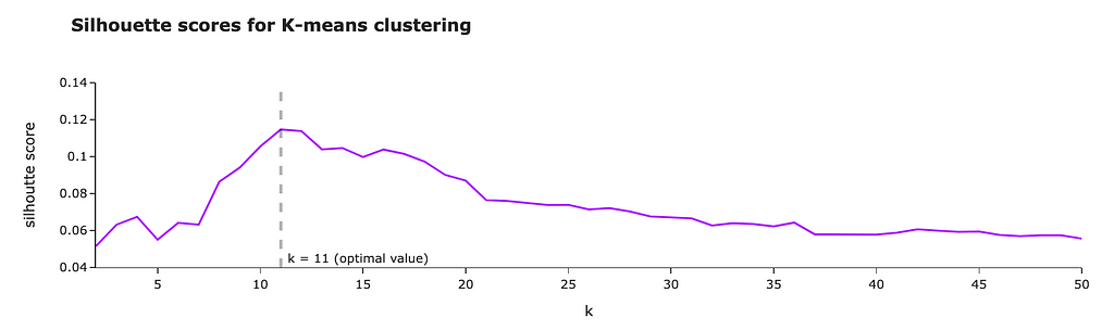
Let’s visualise the clusters using t-SNE for dimensionality reduction as we already did before.
tsne_model = TSNE(n_components=2, random_state=42)
tsne_embeddings_values = tsne_model.fit_transform(embeddings_array)

fig = px.scatter(
    x = tsne_embeddings_values[:,0],
    y = tsne_embeddings_values[:,1],
    color = list(map(lambda x: 'cluster %s' % x, kmeans_labels)),
    hover_name = df.full_text.values,
    title = 't-SNE embeddings for clustering', width = 800, height = 600,
    color_discrete_sequence = plotly.colors.qualitative.Alphabet_r
)
fig.update_layout(
    xaxis_title = 'first component',
    yaxis_title = 'second component')
fig.show()
Visually, we can see that the algorithm was able to define clusters quite well — they are separated pretty well.
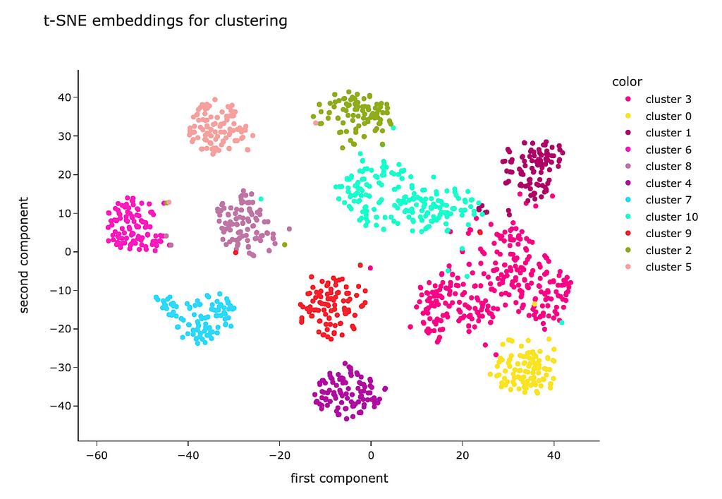
We have factual topic labels, so we can even assess how good clusterisation is. Let’s look at the topics’ mixture for each cluster.
df['cluster'] = list(map(lambda x: 'cluster %s' % x, kmeans_labels))
cluster_stats_df = df.reset_index().pivot_table(
    index = 'cluster', values = 'id',
    aggfunc = 'count', columns = 'topic').fillna(0).applymap(int)

cluster_stats_df = cluster_stats_df.apply(
  lambda x: 100*x/cluster_stats_df.sum(axis = 1))

fig = px.imshow(
    cluster_stats_df.values,
    x = cluster_stats_df.columns,
    y = cluster_stats_df.index,
    text_auto = '.2f', aspect = "auto",
    labels=dict(x="cluster", y="fact topic", color="share, %"),
    color_continuous_scale='pubugn',
    title = '<b>Share of topics in each cluster</b>', height = 550)

fig.show()
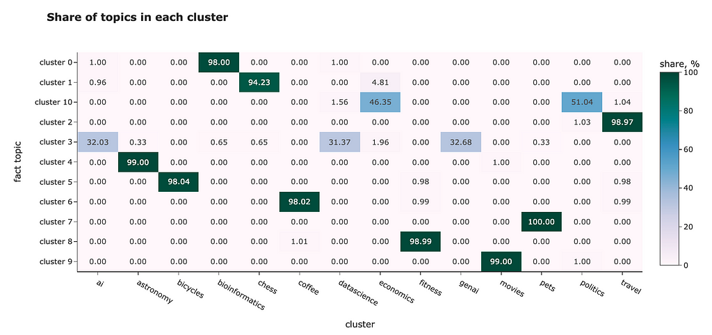
In most cases, clusterisation worked perfectly. For example, cluster 5 contains almost only questions about bicycles, while cluster 6 is about coffee. However, it wasn’t able to distinguish close topics:
We used only embeddings as the features in this example, but if you have any additional information (for example, age, gender or country of the user who asked the question), you can include it in the model, too.
We can use embeddings for classification or regression tasks. For example, you can do it to predict customer reviews’ sentiment (classification) or NPS score (regression).
Since classification and regression are supervised learning, you will need to have labels. Luckily, we know the topics for our questions and can fit a model to predict them.
I will use a Random Forest Classifier. If you need a quick refresher about Random Forests, you can find it here. To assess the classification model’s performance correctly, we will split our dataset into train and test sets (80% vs 20%). Then, we can train our model on a train set and measure the quality on a test set (questions that the model hasn’t seen before).
from sklearn.ensemble import RandomForestClassifier
from sklearn.model_selection import train_test_split
class_model = RandomForestClassifier(max_depth = 10)

# defining features and target
X = embeddings_array
y = df.topic

# splitting data into train and test sets
X_train, X_test, y_train, y_test = train_test_split(
    X, y, random_state = 42, test_size=0.2, stratify=y
)

# fit & predict
class_model.fit(X_train, y_train)
y_pred = class_model.predict(X_test)
To estimate the model’s performance, let’s calculate a confusion matrix. In an ideal situation, all non-diagonal elements should be 0.
from sklearn.metrics import confusion_matrix
cm = confusion_matrix(y_test, y_pred)

fig = px.imshow(
  cm, x = class_model.classes_,
  y = class_model.classes_, text_auto='d',
  aspect="auto",
  labels=dict(
      x="predicted label", y="true label",
      color="cases"),
  color_continuous_scale='pubugn',
  title = '<b>Confusion matrix</b>', height = 550)

fig.show()
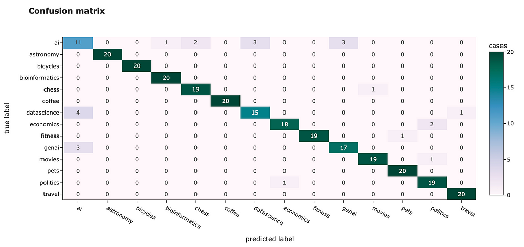
We can see similar results to clusterisation: some topics are easy to classify, and accuracy is 100%, for example, “bicycles” or “travel”, while some others are difficult to distinguish (especially “ai”).
However, we achieved 91.8% overall accuracy, which is quite good.
We can also use embedding to find anomalies in our data. For example, at the t-SNE graph, we saw that some questions are pretty far from their clusters, for instance, for the “travel” topic. Let’s look at this theme and try to find anomalies. We will use the Isolation Forest algorithm for it.
from sklearn.ensemble import IsolationForest

topic_df = df[df.topic == 'travel']
topic_embeddings_array = np.array(topic_df.embedding.values.tolist())

clf = IsolationForest(contamination = 0.03, random_state = 42)
topic_df['is_anomaly'] = clf.fit_predict(topic_embeddings_array)

topic_df[topic_df.is_anomaly == -1][['full_text']]
So, here we are. We’ve found the most uncommon comment for the travel topic (source).
Is it safe to drink the water from the fountains found all over
the older parts of Rome?

When I visited Rome and walked around the older sections, I saw many
different types of fountains that were constantly running with water.
Some went into the ground, some collected in basins, etc.

Is the water coming out of these fountains potable? Safe for visitors
to drink from? Any etiquette regarding their use that a visitor
should know about?
Since it talks about water, the embedding of this comment is close to the coffee topic where people also discuss water to pour coffee. So, the embedding representation is quite reasonable.
We could find it on our t-SNE visualisation and see that it’s actually close to the coffee cluster.
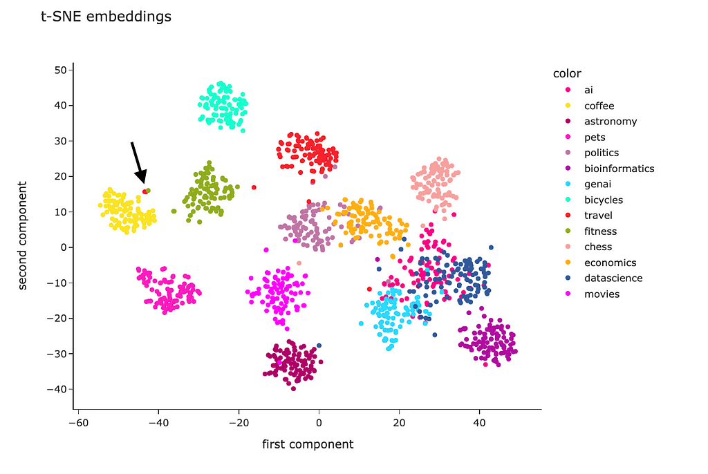
With the recently increased popularity of LLMs, embeddings have been broadly used in RAG use cases.
We need Retrieval Augmented Generation when we have a lot of documents (for example, all the questions from Stack Exchange), and we can’t pass them all to an LLM because
To be able to work with an extensive knowledge base, we can leverage the RAG approach:
To learn more about RAG, don’t hesitate to read my article with much more details here.
In this article, we’ve discussed text embeddings in much detail. Hopefully, now you have a complete and deep understanding of this topic. Here’s a quick recap of our journey:
Thank you a lot for reading this article. If you have any follow-up questions or comments, please leave them in the comments section.
In this article, I used a dataset from Stack Exchange Data Dump, which is available under the Creative Commons license.
This article was inspired by the following courses:
Text Embeddings: Comprehensive Guide was originally published in Towards Data Science on Medium, where people are continuing the conversation by highlighting and responding to this story.
Originally appeared here:
Text Embeddings: Comprehensive Guide
Go Here to Read this Fast! Text Embeddings: Comprehensive Guide


Understanding EMD through theory and from-scratch calculation
Originally appeared here:
Comparison of Distributions with Earth Mover’s Distance
Go Here to Read this Fast! Comparison of Distributions with Earth Mover’s Distance