
Originally appeared here:
Master Dispersion Plots in 6 Minutes!
Go Here to Read this Fast! Master Dispersion Plots in 6 Minutes!
Retrieval-Augmented Generation (RAG) adds a retrieval step to the workflow of an LLM, enabling it to query relevant data from additional sources like private documents when responding to questions and queries [1]. This workflow does not require costly training or fine-tuning of LLMs on the additional documents. The documents are split into snippets, which are then indexed, often using a compact ML-generated vector representation (embedding). Snippets with similar content will be in proximity to each other in this embedding space.
The RAG application projects the user-provided questions into the embedding space to retrieve relevant document snippets based on their distance to the question. The LLM can use the retrieved information to answer the query and to substantiate its conclusion by presenting the snippets as references.
The evaluation of a RAG application is challenging [2]. Different approaches exist: on one hand, there are methods where the answer as ground truth must be provided by the developer; on the other hand, the answer (and the question) can also be generated by another LLM. One of the largest open-source systems for LLM-supported answering is Ragas [4](Retrieval-Augmented Generation Assessment), which provides
In this article, you will learn
Start a notebook and install the required python packages
!pip install langchain langchain-openai chromadb renumics-spotlight
%env OPENAI_API_KEY=<your-api-key>
This tutorial uses the following python packages:
Disclaimer: The author of this article is also one of the developers of Spotlight.
You can use your own RAG Application, skip to the next part to learn how to evaluate, extract and visualize.
Or you can use the RAG application from the last article with our prepared dataset of all Formula One articles of Wikipedia. There you can also insert your own Documents into a ‘docs/’ subfolder.
This dataset is based on articles from Wikipedia and is licensed under the Creative Commons Attribution-ShareAlike License. The original articles and a list of authors can be found on the respective Wikipedia pages.
Now you can use Langchain’s DirectoryLoader to load all files from the docs subdirectory and split the documents in snippets using the RecursiveCharacterTextSpliter. With OpenAIEmbeddings you can create embeddings and store them in a ChromaDB as vector store. For the Chain itself you can use LangChains ChatOpenAI and a ChatPromptTemplate.
The linked code for this article contains all necessary steps and you can find a detailed description of all steps above in the last article.
One important point is, that you should use a hash function to create ids for snippets in ChromaDB. This allows to find the embeddings in the db if you only have the document with its content and metadata. This makes it possible to skip documents that already exist in the database.
import hashlib
import json
from langchain_core.documents import Document

def stable_hash_meta(doc: Document) -> str:
    """
    Stable hash document based on its metadata.
    """
    return hashlib.sha1(json.dumps(doc.metadata, sort_keys=True).encode()).hexdigest()

...
splits = text_splitter.split_documents(docs)
splits_ids = [
    {"doc": split, "id": stable_hash_meta(split.metadata)} for split in splits
]

existing_ids = docs_vectorstore.get()["ids"]
new_splits_ids = [split for split in splits_ids if split["id"] not in existing_ids]

docs_vectorstore.add_documents(
    documents=[split["doc"] for split in new_splits_ids],
    ids=[split["id"] for split in new_splits_ids],
)
docs_vectorstore.persist()
For a common topic like Formula One, one can also use ChatGPT directly to generate general questions. In this article, four methods of question generation are used:
from ragas.testset import TestsetGenerator

generator = TestsetGenerator.from_default(
    openai_generator_llm="gpt-3.5-turbo-16k",
    openai_filter_llm="gpt-3.5-turbo-16k"
)

testset_ragas_gpt35 = generator.generate(docs, 100)
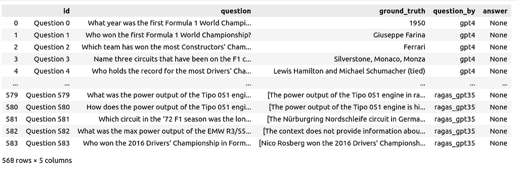
The questions and answers were not reviewed or modified in any way. All questions are combined in a single dataframe with the columns id, question, ground_truth, question_by and answer.
Next, the questions will be posed to the RAG system. For over 500 questions, this can take some time and incur costs. If you ask the questions row-by-row, you can pause and continue the process or recover from a crash without losing the results so far:
for i, row in df_questions_answers.iterrows():
    if row["answer"] is None or pd.isnull(row["answer"]):
        response = rag_chain.invoke(row["question"])

        df_questions_answers.loc[df_questions_answers.index[i], "answer"] = response[
            "answer"
        ]
        df_questions_answers.loc[df_questions_answers.index[i], "source_documents"] = [
            stable_hash_meta(source_document.metadata)
            for source_document in response["source_documents"]
        ]
Not only is the answer stored but also the source IDs of the retrieved document snippets, and their text content as context:
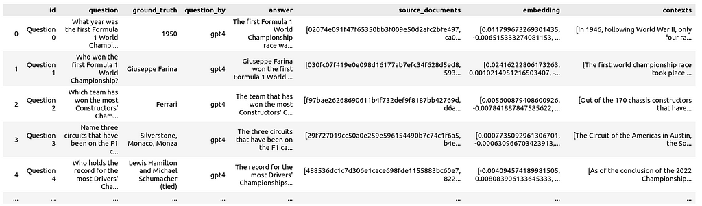
Additionally, the embeddings for all questions are generated and stored in the dataframe as well. This allows for visualizing them alongside the documents.
Ragas provides metrics for evaluating each component of your RAG pipeline in isolation and end-to-end metrics for overall performance:
For now, we focus on the end-to-end metric of answer correctness. The column names and content in the dataframe are copied and adapted to meet the naming and formatting requirements according to the Ragas API:
# prepare the dataframe for evaluation
df_qa_eval = df_questions_answers.copy()


# adapt the ground truth to the ragas naming and format
df_qa_eval.rename(columns={"ground_truth": "ground_truths"}, inplace=True)
df_qa_eval["ground_truths"] = [
    [gt] if not isinstance(gt, list) else gt for gt in df_qa_eval["ground_truths"]
]
This again can take some time and even more money than just querying your RAG system. Let’s apply the evaluation row-by-row to be able to recover from a crash without losing the results so far:
# evaluate the answer correctness if not already done
fields = ["question", "answer", "contexts", "ground_truths"]
for i, row in df_qa_eval.iterrows():
    if row["answer_correctness"] is None or pd.isnull(row["answer_correctness"]):
        evaluation_result = evaluate(
            Dataset.from_pandas(df_qa_eval.iloc[i : i + 1][fields]),
            [answer_correctness],
        )
        df_qa_eval.loc[i, "answer_correctness"] = evaluation_result[
            "answer_correctness"
        ]
Afterwards, you can store the results in the df_questions_answer dataframe:
df_questions_answers["answer_correctness"] = df_qa_eval["answer_correctness"]
To include the document snippets in the visualization, we add references from documents to questions that used the document as a source. Additionally, the count of questions referencing a document is stored:
# Explode 'source_documents' so each document ID is in its own row alongside the question ID
df_questions_exploded = df_qa_eval.explode("source_documents")

# Group by exploded 'source_documents' (document IDs) and aggregate
agg = (
    df_questions_exploded.groupby("source_documents")
    .agg(
        num_questions=("id", "count"),  # Count of questions referencing the document
        question_ids=(
            "id",
            lambda x: list(x),
        ),  # List of question IDs referencing the document
    )
    .reset_index()
    .rename(columns={"source_documents": "id"})
)

# Merge the aggregated information back into df_documents
df_documents_agg = pd.merge(df_docs, agg, on="id", how="left")

# Use apply to replace NaN values with empty lists for 'question_ids'
df_documents_agg["question_ids"] = df_documents_agg["question_ids"].apply(
    lambda x: x if isinstance(x, list) else []
)
# Replace NaN values in 'num_questions' with 0
df_documents_agg["num_questions"] = df_documents_agg["num_questions"].fillna(0)
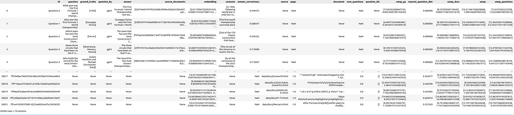
Now concatenate the dataframe of questions with the dataframe of the documents
df = pd.concat([df_qa_eval, df_documents_agg], axis=0)
Additionally, let’s prepare some different UMAP [3] mappings. You could do much the same in the Spotlight GUI later, but doing it upfront can save time.
We prepare each of the UMAP transformations like this:
umap = UMAP(n_neighbors=20, min_dist=0.15, metric="cosine", random_state=42).fit
umap_all = umap.transform(df["embedding"].values.tolist())
df["umap"] = umap_all.tolist()
Another interesting metric for each of the document snippets is the distance between its embeddings and the embeddings of the nearest question
question_embeddings = np.array(df[df["question"].notna()]["embedding"].tolist())
df["nearest_question_dist"] = [  # brute force, could be optimized using ChromaDB
    np.min([np.linalg.norm(np.array(doc_emb) - question_embeddings)])
    for doc_emb in df["embedding"].values
]
This metric can be helpful to find documents that are not referenced by questions.
If you skipped the previous steps, you can download the dataframe and load it with:
import pandas as pd
df = pd.read_parquet("df_f1_rag_docs_and_questions.parquet")
and start Renumics Spotlight to visualize it with:
from renumics import spotlight

spotlight.show(df)
spotlight.show(
    df,
    layout="/home/markus/Downloads/layout_rag_1.json",
    dtype={x: Embedding for x in df.keys() if "umap" in x},
)
It will open a new brwoser window:
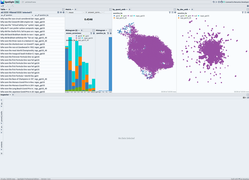
On the top left side, you can see a table of all questions and all document snippets. You can use the “visible columns” button to control which columns of the dataframe are shown in the table. It is useful to create a filter directly that selects only the questions to be able to turn the questions on and off in the visualizations: Select all questions and and then create a filter using the “Create filter from selected row” button.
To the right of the table, the answer correctness is displayed as a metric across all questions. Below there are two histograms; the left one shows the distribution of answer correctness divided into the different methods of question generation. The right one shows the distribution of methods of question generation. Here, it is advisable to create a filter for the questions using the filter button to display only the selected rows (the questions) if needed.
On the right side, there are two similarity maps. The first one uses the umap_questions column and shows the questions and documents based on the transformation applied only to the questions. It is helpful for viewing the distribution of questions independently from the associated documents because this approach allows analysts to identify patterns or clusters within the questions themselves.
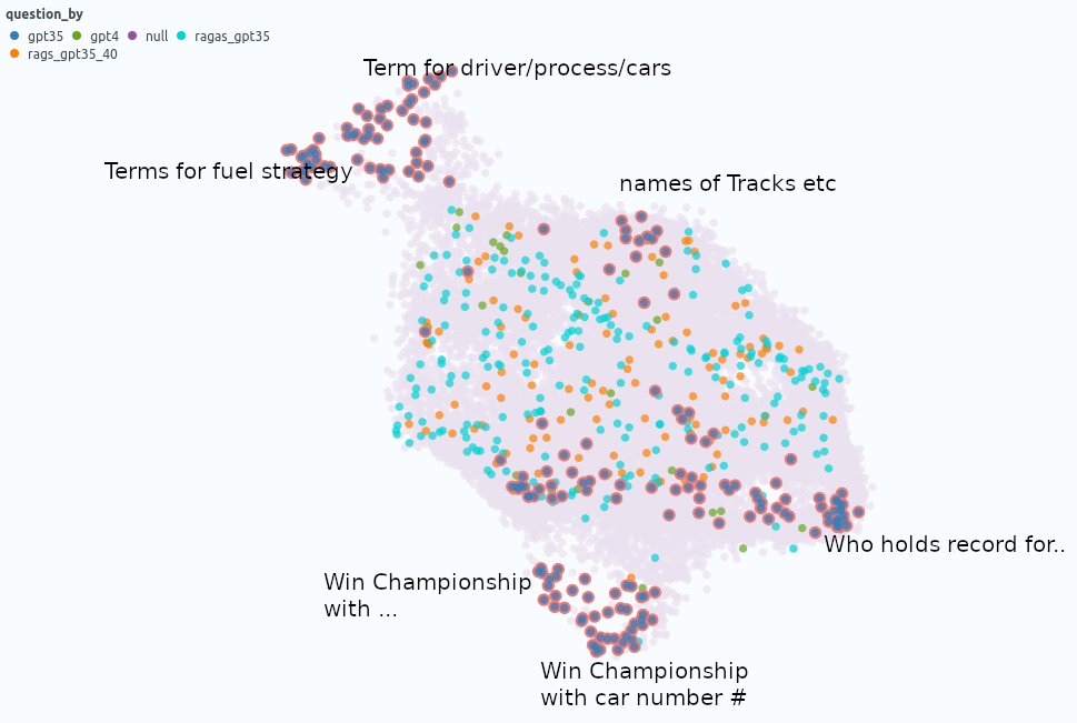
The second similarity map shows the questions and documents based on the transformation applied only to the documents (umap_docs). It is useful for viewing the questions in the context of their associated documents. A similarity map that simultaneously transforms questions and documents has proven to be less helpful with a larger number of questions, as more or fewer questions get clustered together and tend to be separated from the documents. Therefore, this representation is omitted here.
In the similarity map umap_docs, you can identify areas in the embedding space of the documents that have no neighboring questions. It is even better recognized when selecting nearest_question_dist for coloring.
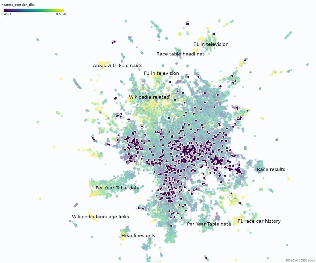
Some clusters can be identified, including snippets that contain only headings or tabular data containing only numbers page by page, whose meaning is lost during splitting. Additionally, many Wikipedia-specific text additions that contain no relevant information, such as links to other languages or editing notes, form clusters with no neighboring questions.
Removing the noise in form of Wikipedia-related text is very simple when using the Wikipedia API. It is probably not particularly necessary, as it mainly costs some space — it is not expected that the RAG result will be particularly worsened by it. However, data contained in large tables are hardly captured by the RAG system and it could ne benifical to extract these using advanced pre-processing methods for Table Extraction and to connect them to the RAG system.
Another point that you can observe in the umap_docs similarity map is how the questions from different sources are distributed.
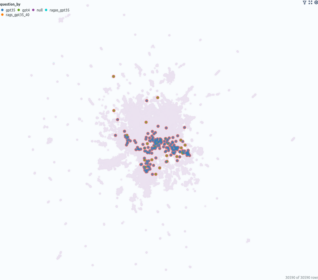
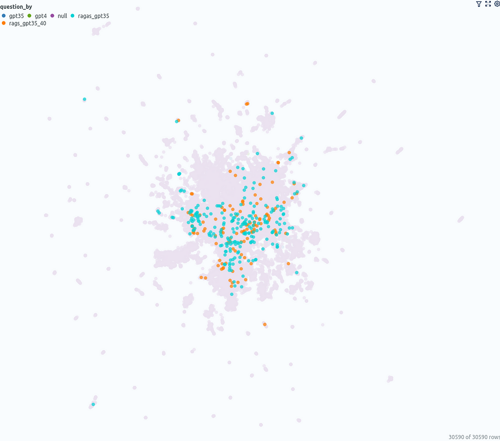
The questions that were directly generated by ChatGPT (GPT-3.5, GPT-4) are located in a more confined area in the center, whereas the questions generated with ragas based on the documents cover a larger area.
The histogram can be used as a starting point to get an initial impression of the global statistics of the data. Overall, across all questions, the answer correctness is 0.45. For the questions created without ragas, it is 0.36, and for questions with ragas, it is 0.52. It was expected that the system would perform better for questions generated by ragas, as these questions are based on the available data, whereas the questions directly generated by ChatGPT could come from all the data with which ChatGPT was trained.
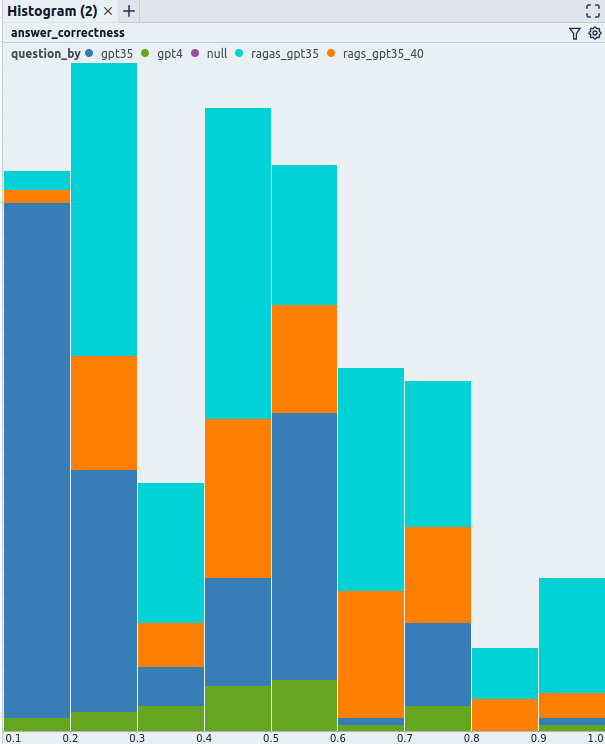
A quick, random manual review of some of the questions/answers and ground truth shows that in the interval ofanswer correctness0.3–0.4, most questions were still correctly answered according to the ground truth. In the interval 0.2–0.3, many incorrect answers are present. In the interval 0.1–0.2, most answers are incorrect. Notably, almost all questions in this range came from GPT-3.5. The two questions in this interval generated with GPT-4 were answered correctly even though they received an answer correctness of below 0.2.
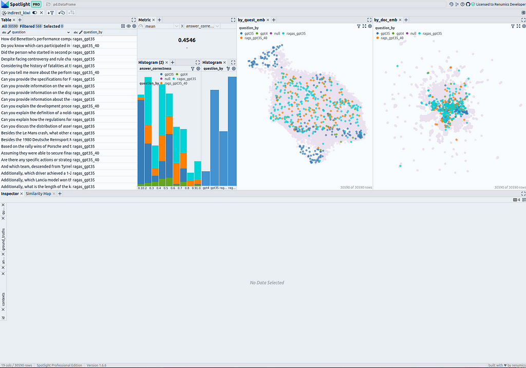
The Questions Embedding Similarity Map can be helpful to dig deeper into answer correctness by examining clusters of similar questions that may cause similar problems.
In conclusion, utilizing UMAP-based visualizations offers a interesting approach to dig deeper than just analyzing global metrics. The document embedding similarity map gives a good overview, illustrating the clustering of similar documents and their relation to evaluation questions. The question similarity map reveals patterns that allow the differentiation and analysis of questions in conjunction with quality metrics to enable insight generation. Follow the Visualize results section to apply the visualization on your evaluation strategy — what insights will you uncover?
I am a professional with expertise in creating advanced software solutions for the interactive exploration of unstructured data. I write about unstructured data and use powerful visualization tools to analyze and make informed decisions.
[1] Yunfan Gao, Yun Xiong, Xinyu Gao, Kangxiang Jia, Jinliu Pan, Yuxi Bi, Yi Dai, Jiawei Sun, Qianyu Guo, Meng Wang, Haofen Wang: Retrieval-Augmented Generation for Large Language Models: A Survey (2024), arxiv
[2] Yixuan Tang, Yi Yang: MultiHop-RAG: Benchmarking Retrieval-Augmented Generation for Multi-Hop Queries (2021), arXiv
[3] Leland McInnes, John Healy, James Melville: UMAP: Uniform Manifold Approximation and Projection for Dimension Reduction (2018), arXiv
[4] Shahul Es, Jithin James, Luis Espinosa-Anke, Steven Schockaert: RAGAS: Automated Evaluation of Retrieval Augmented Generation (2023), arXiv
Visualize your RAG Data — Evaluate your Retrieval-Augmented Generation System with Ragas was originally published in Towards Data Science on Medium, where people are continuing the conversation by highlighting and responding to this story.
Originally appeared here:
Visualize your RAG Data — Evaluate your Retrieval-Augmented Generation System with Ragas
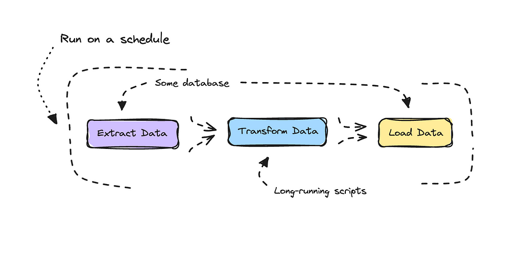

ETL stands for Extract, Transform, and Load. An ETL pipeline is essentially just a data transformation process — extracting data from one place, doing something with it, and then loading it back to the same or a different place.
If you are working with natural language processing via APIs, which I’m guessing most will start doing, you can easily hit the timeout threshold of AWS Lambda when processing your data, especially if at least one function exceeds 15 minutes. So, while Lambda is great because it’s quick and really cheap, the timeout can be a bother.
The choice here is to deploy your code as a container that has the option of running as long as it needs to and run it on a schedule. So, instead of spinning up a function as you do with Lambda, we can spin up a container to run in an ECS cluster using Fargate.

For clarification, Lambda, ECS and EventBridge are all AWS Services.
Just as with Lambda, the cost of running a container for an hour or two is minimal. However, it’s a bit more complicated than running a serverless function. But if you’re reading this, then you’ve probably run into the same issues and are wondering what the easiest way to transition is.
I have created a very simple ETL template that uses Google BigQuery to extract and load data. This template will get you up and running within a few minutes if you follow along.
Using BigQuery is entirely optional but I usually store my long term data there.
Instead of building something complex here, I will show you how to build something minimal and keep it really lean.
If you don’t need to process data in parallel, you shouldn’t need to include something like Airflow. I’ve seen a few articles out there that unnecessarily set up complex workflows, which aren’t strictly necessary for straightforward data transformation.
Besides, if you feel like you want to add on to this later, that option is yours.
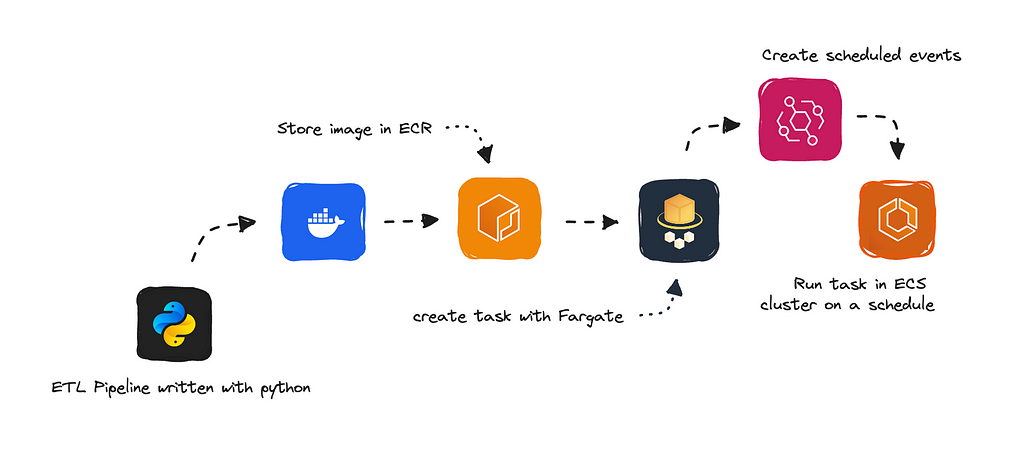
We’ll build our script in Python as we’re doing data transformation, then bundle it up with Docker and push it to an ECR repository.
From here, we can create a task definition using AWS Fargate and run it on a schedule in an ECS cluster.
Don’t worry if this feels foreign; you’ll understand all these services and what they do as we go along.
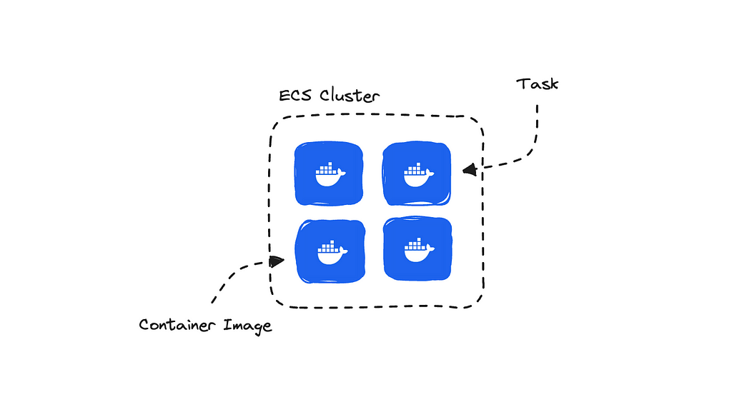
If you are new to working with containers, then think of ECS (Elastic Container Service) as something that helps us set up an environment where we can run one or more containers simultaneously.
Fargate, on the other hand, helps us simplify the management and setup of the containers themselves using Docker images — which are referred to as tasks in AWS.
There is the option of using EC2 to set up your containers, but you would have to do a lot more manual work. Fargate manages the underlying instances for us, whereas with EC2, you are required to manage and deploy your own compute instances. Hence, Fargate is often referred to as the ‘serverless’ option.
I found a thread on Reddit discussing this, if you’re keen to read a bit about how users find using EC2 versus Fargate. It can give you an idea of how people compare EC2 and Fargate.
Not that I’m saying Reddit is the source of truth, but it’s useful for getting a sense of user perspectives.
The primary concern I usually have is to keep the code running efficiently while also managing the total cost.
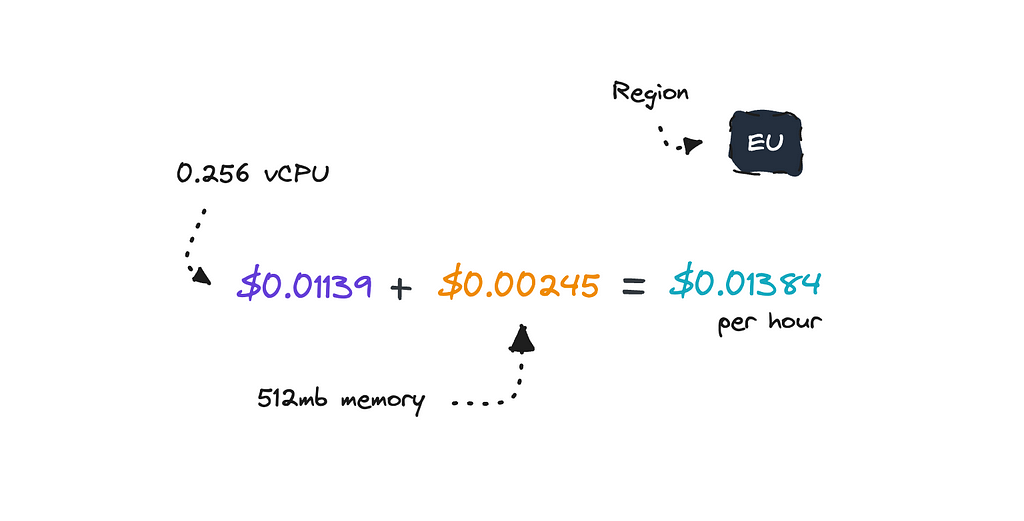
As we’re only running the container when we need to, we only pay for the amount of resources we use. The price we pay is determined by several factors, such as the number of tasks running, the execution duration of each task, the number of virtual CPUs (vCPUs) used for the task, and memory usage.
But to give you a rough idea, on a high level, the total cost for running one task is around $0.01384 per hour for the EU region, depending on the resources you’ve provisioned.
If we were to compare this price with AWS Glue we can get a bit of perspective if it is good or not.
If an ETL job requires 4 DPUs (the default number for an AWS Glue job) and runs for an hour, it would cost 4 DPUs * $0.44 = $1.76. This cost is for only one hour and is significantly higher than running a simple container.
This is, of course, a simplified calculation, and the actual number of DPUs can vary depending on the job. You can check out AWS Glue pricing in more detail on their pricing page.
To run long-running scripts, setting up your own container and deploying it on ECS with Fargate makes sense, both in terms of efficiency and cost.
To follow this article, I’ve created a simple ETL template to help you get up and running quickly.
This template uses BigQuery to extract and load data. It will extract a few rows, do something simple and then load it back to BigQuery.
When I run my pipelines I have other things that transform data — I use APIs for natural language processing that runs for a few hours in the morning — but that is up to you to add on later. This is just to give you a template that will be easy to work with.
To follow along this tutorial, the main steps will be as follows:
In total it shouldn’t take you longer than 20 minutes to get through this, using the code I’ll provide you with. This assumes you have an AWS account ready, and if not, add on 5 to 10 minutes.
First create a new folder locally and locate into it.
mkdir etl-pipelines
cd etl-pipelines
Make sure you have python installed.
python --version
If not, install it locally.
Once you’re ready, you can go ahead and clone the template I have already set up.
git clone https://github.com/ilsilfverskiold/etl-pipeline-fargate.git
When it has finished fetching the code, open it up in your code editor.
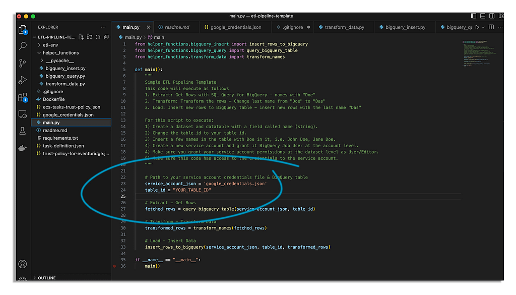
First check the main.py file to look how I’ve structured the code to understand what it does.
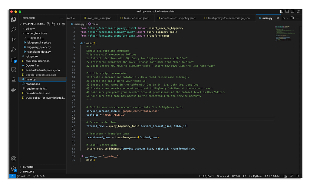
Essentially, it will fetch all names with “Doe” in it from a table in BigQuery that you specify, transform these names and then insert them back into the same data table as new rows.
You can go into each helper function to see how we set up the SQL Query job, transform the data and then insert it back to the BigQuery table.
The idea is of course that you set up something more complex but this is a simple test run to make it easy to tweak the code.
If you want to continue with the code I’ve prepared you will need to set up a few things in BigQuery. Otherwise you can skip this part.
Here are the things you will need:
To get a service account you will need to navigate to IAM in the Google Cloud Console and then to Service Accounts.
Once there, create a new service account.
Once it has been created, you will need to give your service account BigQuery User access globally via IAM.
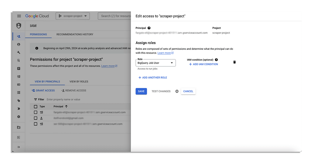
You will also have to give this service account access to the dataset itself which you do in BigQuery directly via the dataset’s Share button and then by pressing Add Principal.

After you’ve given the user the appropriate permissions, make sure you go back to the Service Accounts and then download a key. This will give you a json file that you need to put in your root folder.

Now, the most important part is making sure the code has access to the google credentials and is using the correct data table.
You’ll want the json file you’ve downloaded with the Google credentials in your root folder as google_credentials.json and then you want to specify the correct table ID.
Now you might argue that you do not want to store your credentials locally which is only right.
You can add in the option of storing your json file in AWS Secrets Manager later. However, to start, this will be easier.
We’ll run this code locally first, just so we can see that it works.
So, set up a Python virtual environment and activate it.
python -m venv etl-env
source etl-env/bin/activate  # On Windows use `venvScriptsactivate`
Then install dependencies. We only have google-cloud-bigquery in there but ideally you will have more dependencies.
pip install -r requirements.txt
Run the main script.
python main.py
This should log ‘New rows have been added’ in your terminal. This will then confirm that the code works as we’ve intended.
Now to push this code to ECS we will have to bundle it up into a Docker image which means that you will need Docker installed locally.
If you do not have Docker installed, you can download it here.
Docker helps us package an application and its dependencies into an image, which can be easily recognized and run on any system. Using ECS, it’s required of us to bundle our code into Docker images, which are then referenced by a task definition to run as containers.
I have already set up a Dockerfile in your folder. You should be able to look into it there.
FROM --platform=linux/amd64 python:3.11-slim

WORKDIR /app

COPY . /app

RUN pip install --no-cache-dir -r requirements.txt

CMD ["python", "main.py"]
As you see, I’ve kept this really lean as we’re not connecting web traffic to any ports here.
We’re specifying AMD64 which you may not need if you are not on a Mac with an M1 chip but it shouldn’t hurt. This will specify to AWS the architecture of the docker image so we don’t run into compatibility issues.
When working with AWS, access will need to be specified. Most of the issues you’ll run into are permission issues. We’ll be working with the CLI locally, and for this to work we’ll have to create an IAM user that will need quite broad permissions.
Go to the AWS console and then navigate to IAM. Create a new user, add permissions and then create a new policy to attach to it.
I have specified the permissions needed in your code in the aws_iam_user.json file. You’ll see a short snippet below of what this json file looks like.
{
 "Version": "2012-10-17",
 "Statement": [
  {
   "Sid": "VisualEditor0",
   "Effect": "Allow",
   "Action": [
    "logs:CreateLogGroup",
    "iam:CreateRole",
    "iam:AttachRolePolicy",
    "iam:PutRolePolicy",
    "ecs:DescribeTaskDefinition",
    ...more
   ],
   "Resource": "*"
  }
 ]
}
You’ll need to go into this file to get all the permissions you will need to set, this is just a short snippet. I’ve set it to quite a few, which you may want to tweak to your own preferences later.
Once you’ve created the IAM user and you’ve added the correct permissions to it, you will need to generate an access key. Choose ‘Command Line Interface (CLI)’ when asked about your use case.
Download the credentials. We’ll use these to authenticate in a bit.
Next, we’ll connect our terminal to our AWS account.
If you don’t have the CLI set up yet you can follow the instructions here. It is really easy to set this up.
Once you’ve installed the AWS CLI you’ll need to authenticate with the IAM user we just created.
aws configure
Use the credentials we downloaded from the IAM user in the previous step.
Now, we can get started with the DevOps of it all.
We’ll first need to create a repository in Elastic Container Registry. ECR is where we can store and manage our docker images. We’ll be able to reference these images from ECR when we set up our task definitions.
To create a new ECR repository run this command in your terminal. This will create a repository called bigquery-etl-pipeline.
aws ecr create-repository — repository-name bigquery-etl-pipeline
Note the repository URI you get back.
From here we have to build the docker image and then push this image to this repository.
To do this you can technically go into the AWS console and find the ECR repository we just created. Here AWS will let us see the entire push commands we need to run to authenticate, build and push our docker image to this ECR repository.
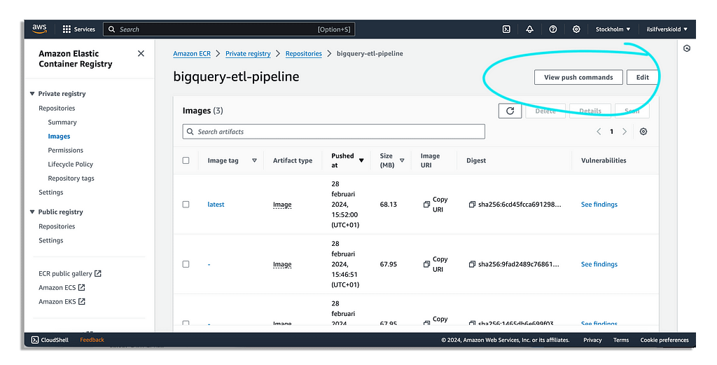
However, if you are on a Mac I would advice you to specify the architecture when building the docker image or you may run into issues.
If you are following along with me, then start with authenticating your docker client like so.
aws ecr get-login-password --region YOUR_REGION | docker login --username AWS --password-stdin YOUR_ACCOUNT_ID.dkr.ecr.YOUR_REGION.amazonaws.com
Be sure to change the values, region and account ID where applicable.
Build the docker image.
docker buildx build --platform=linux/amd64 -t bigquery-etl-pipeline .
This is where I have tweaked the command to specify the linux/amd64 architecture.
Tag the docker image.
docker tag bigquery-etl-pipeline:latest YOUR_ACCOUNT_ID.dkr.ecr.YOUR_REGION.amazonaws.com/bigquery-etl-pipeline:latest
Push the docker image.
docker push YOUR_ACCOUNT_ID.dkr.ecr.YOUR_REGION.amazonaws.com/bigquery-etl-pipeline:latest
If everything worked as planned you’ll see something like this in your terminal.
9f691c4f0216: Pushed
ca0189907a60: Pushed
687f796c98d5: Pushed
6beef49679a3: Pushed
b0dce122021b: Pushed
4de04bd13c4a: Pushed
cf9b23ff5651: Pushed
644fed2a3898: Pushed
Now that we have pushed the docker image to an ECR repository, we can use it to set up our task definition using Fargate.
If you run into EOF issues here it is most likely related to IAM permissions. Be sure to give it everything it needs, in this case full access to ECR to tag and push the image.
Remember what I told you before, the biggest issues you’ll run into in AWS pertains to roles between different services.
For this to flow neatly we’ll have to make sure we set up a few things before we start setting up a task definition and an ECS cluster.
To do this, we first have to create a task role — this role is the role that will need access to services in the AWS ecosystem from our container — and then the execution role — so the container will be able to pull the docker image from ECR.
aws iam create-role --role-name etl-pipeline-task-role --assume-role-policy-document file://ecs-tasks-trust-policy.json
aws iam create-role - role-name etl-pipeline-execution-role - assume-role-policy-document file://ecs-tasks-trust-policy.json
I have specified a json file called ecs-tasks-trust-policy.json in your folder locally that it will use to create these roles.
For the script that we are pushing, it won’t need to have permission to access other AWS services so for now there is no need to attach policies to the task role. Nevertheless, you may want to do this later.
However, for the execution role though we will need to give it ECR access to pull the docker image.
To attach the policy AmazonECSTaskExecutionRolePolicy to the execution role run this command.
aws iam attach-role-policy --role-name etl-pipeline-execution-role --policy-arn arn:aws:iam::aws:policy/service-role/AmazonECSTaskExecutionRolePolicy
We also create one last role while we’re at it, a service role.
aws iam create-service-linked-role - aws-service-name ecs.amazonaws.com
If you don’t create the service role you may end up with an errors such as ‘Unable to assume the service linked role. Please verify that the ECS service linked role exists’ when you try to run a task.
The last thing we create a log group. Creating a log group is essential for capturing and accessing logs generated by your container.
To create a log group you can run this command.
aws logs create-log-group - log-group-name /ecs/etl-pipeline-logs
Once you’ve created the execution role, the task role, the service role and then the log group we can continue to set up the ECS task definition.
A task definition is a blueprint for your tasks, specifying what container image to use, how much CPU and memory is needed, and other configurations. We use this blueprint to run tasks in our ECS cluster.
I have already set up the task definition in your code at task-definition.json. However, you need to set your account id as well as region in there to make sure it runs as it should.
{
    "family": "my-etl-task",
    "taskRoleArn": "arn:aws:iam::ACCOUNT_ID:role/etl-pipeline-task-role",
    "executionRoleArn": "arn:aws:iam::ACCOUNT_ID:role/etl-pipeline-execution-role",
    "networkMode": "awsvpc",
    "containerDefinitions": [
        {
            "name": "my-etl-container",
            "image": "ACCOUNT_ID.dkr.ecr.REGION.amazonaws.com/bigquery-etl-pipeline:latest",
            "cpu": 256,
            "memory": 512,
            "essential": true,
            "logConfiguration": {
                "logDriver": "awslogs",
                "options": {
                    "awslogs-group": "/ecs/etl-pipeline-logs",
                    "awslogs-region": "REGION",
                    "awslogs-stream-prefix": "ecs"
                }
            }
        }
    ],
    "requiresCompatibilities": ["FARGATE"],
    "cpu": "256",
    "memory": "512"
}
Remember the URI we got back when we created the ECR repository? This is where we’ll use it. Remember the execution role, the task role and the log group? We’ll use it there as well.
If you’ve named the ECR repository along with the roles and log group exactly what I named mine then you can simply change the account ID and Region in this json otherwise make sure the URI is the correct one.
You can also set CPU and memory here for what you’ll need to run your task — i.e. your code. I’ve set .25 vCPU and 512 mb as memory.
Once you’re satisfied you can register the task definition in your terminal.
aws ecs register-task-definition --cli-input-json file://task-definition.json
Now you should be able to go into Amazon Elastic Container Service and then find the task we’ve created under Task Definitions.
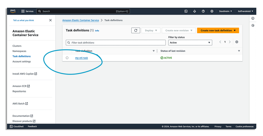
This task — i.e. blueprint — won’t run on it’s own, we need to invoke it later.
An ECS Cluster serves as a logical grouping of tasks or services. You specify this cluster when running tasks or creating services.
To create a cluster via the CLI run this command.
aws ecs create-cluster --cluster-name etl-pipeline-cluster
Once you run this command, you’ll be able to see this cluster in ECS in your AWS console if you look there.
We’ll attach the Task Definition we just created to this cluster when we run it for the next part.
Before we can run the task we need to get ahold of the subnets that are available to us along with a security group id.
We can do this directly in the terminal via the CLI.
Run this command in the terminal to get the available subnets.
aws ec2 describe-subnets
You’ll get back an array of objects here, and you’re looking for the SubnetId for each object.
If you run into issues here, make sure your IAM has the appropriate permissions. See the aws_iam_user.json file in your root folder for the permissions the IAM user connected to the CLI will need. I will stress this, because it’s the main issues that I always run into.
To get the security group ID you can run this command.
aws ec2 describe-security-groups
You are looking for GroupId here in the terminal.
If you got at least one SubnetId and then a GroupId for a security group, we’re ready to run the task to test that the blueprint — i.e. task definition — works.
aws ecs run-task
    --cluster etl-pipeline-cluster
    --launch-type FARGATE
    --task-definition my-etl-task
    --count 1
    --network-configuration "awsvpcConfiguration={subnets=[SUBNET_ID],securityGroups=[SECURITY_GROUP_ID],assignPublicIp=ENABLED}"
Do remember to change the names if you’ve named your cluster and task definition differently. Remember to also set your subnet ID and security group ID.
Now you can navigate to the AWS console to see the task running.

If you are having issues you can look into the logs.
If successful, you should see a few transformed rows added to BigQuery.
Now, we’ve managed to set up the task to run in an ECS cluster. But what we’re interested in is to make it run on a schedule. This is where EventBridge comes in.
EventBridge will set up our scheduled events, and we can set this up using the CLI as well. However, before we set up the schedule we first need to create a new role.
This is life when working with AWS, everything needs to have permission to interact with each other.
In this case, EventBridge will need permission to call the ECS cluster on our behalf.
In the repository you have a file called trust-policy-for-eventbridge.json that I have already put there, we’ll use this file to create this EventBridge role.
Paste this into the terminal and run it.
aws iam create-role
    --role-name ecsEventsRole
    --assume-role-policy-document file://trust-policy-for-eventbridge.json
We then have to attach a policy to this role.
aws iam attach-role-policy
    --role-name ecsEventsRole
    --policy-arn arn:aws:iam::aws:policy/AmazonECS_FullAccess
We need it to at least be able to have ecs:RunTask but we’ve given it full access. If you prefer to limit the permissions, you can create a custom policy with just the necessary permissions instead.
Now let’s set up the rule to schedule the task to run with the task definition every day at 5 am UTC. This is usually the time I’d like for it to process data for me so if it fails I can look into it after breakfast.
aws events put-rule
    --name "ETLPipelineDailyRun"
    --schedule-expression "cron(0 5 * * ? *)"
    --state ENABLED
You should receive back an object with a field called RuleArn here. This is just to confirm that it worked.
Next step is now to associate the rule with the ECS task definition.
aws events put-targets --rule "ETLPipelineDailyRun"
    --targets "[{"Id":"1","Arn":"arn:aws:ecs:REGION:ACCOUNT_NUMBER:cluster/etl-pipeline-cluster","RoleArn":"arn:aws:iam::ACCOUNT_NUMBER:role/ecsEventsRole","EcsParameters":{"TaskDefinitionArn":"arn:aws:ecs:REGION:ACCOUNT_NUMBER:task-definition/my-etl-task","TaskCount":1,"LaunchType":"FARGATE","NetworkConfiguration":{"awsvpcConfiguration":{"Subnets":["SUBNET_ID"],"SecurityGroups":["SECURITY_GROUP_ID"],"AssignPublicIp":"ENABLED"}}}}]"
Remember to set your own values here for region, account number, subnet and security group.
Use the subnets and security group that we got earlier. You can set multiple subnets.
Once you’ve run the command the task is scheduled for 5 am every day and you’ll find it under Scheduled Tasks in the AWS Console.
So keeping your Google credentials in the root folder isn’t ideal, even if you’ve limited access to your datasets for the Google service account.
Here we can add on the option of moving these credentials to another AWS service and then accessing it from our container.
For this to work you’ll have to move the credentials file to Secrets Manager, tweak the code so it can fetch it to authenticate and make sure that the task role has permissions to access AWS Secrets Manager on your behalf.
When you’re done you can simply push the updated docker image to your ECR repo you set up before.
Now you’ve got a very simple ETL pipeline running in a container on AWS on a schedule. The idea is that you add to it to do your own data transformations.
Hopefully this was a useful piece for anyone that is transitioning to setting up their long-running data transformation scripts on ECS in a simple, cost effective and straightforward way.
Let me know if you run into any issues in case there is something I missed to include.
❤
Deploy Long-Running ETL Pipelines to ECS with Fargate was originally published in Towards Data Science on Medium, where people are continuing the conversation by highlighting and responding to this story.
Originally appeared here:
Deploy Long-Running ETL Pipelines to ECS with Fargate
Go Here to Read this Fast! Deploy Long-Running ETL Pipelines to ECS with Fargate


Data engineering techniques for robust and sustainable ETL
Originally appeared here:
Building Durable Data Pipelines

This project utilizes a scenario based qualitative stress testing approach to identify US coastal census tracts expected to adversely impacted by sea level rise (SLR) in the medium (2050) and long term (2100). One Baseline and two ‘plausible but severe’ Adverse scenarios were designed covering 1–7ft of sea level rise.
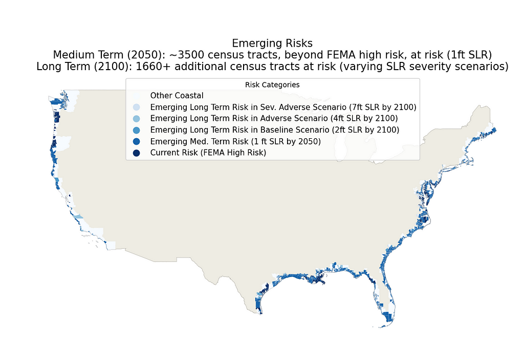
The key observations through this analysis were that that outside of current FEMA high risk areas, there are ~3500 other census tracts along the contiguous US coastline that are expected to experience an average SLR increase of 1ft in the medium term (by 2050). Longer term (by 2100) an additional ~1660 census tracts are at risk for 2–7ft of SLR. The observations for the medium term are particularly important given that they are expected to materialize irrespective of future emissions pathways or other climate mitigation action due the warming of the ocean that has already occurred due to climate change³.
This project predominantly utilizes Python data analysis libraries, e.g., pandas and geopandas as well as some visualization libraries, e.g., matplotlib, seaborn. The code for this project can be found here. The data for this project has predominantly been sourced from the US census bureau and from NOAA. Further details can be found in Technology and Data section below
About 40% of the US population, or ~128 million people, reside in coastal counties¹. While residential assets in general have been battered by a slew of extreme weather events in recent years, e.g., hurricanes, wildfires etc., for these coastal residents, another significant emerging risk is flooding and property loss due to accelerated sea level rise (SLR). However, in the exploratory research for this project, it was found that there may not yet be a deep understanding of the full extend of potential SLR impacts. Therefore, this project intends to bring awareness to regions expected to be impacted in the medium term (2050) and longer term (2100) in various scenarios of accelerated sea level rise.
The National Oceanic and Atmospheric Administration (NOAA) is a leading US scientific agency charged with monitoring oceanic and atmospheric conditions². Per NOAA’s 2022 Sea Level Rise Technical Report³, sea levels are currently rising at a significantly accelerated pace compared to previously observed levels in the 20th century: sea levels along the contiguous US coastline are expected to rise, on average, as much over the next 30 years (2020–2050) as they have over the last 100 years (1920–2020).
Over the long term (by 2100), SLR projections along the contiguous US coastline vary between 2–7ft on average compared to 2000 levels. The variability in these projections is mainly due to uncertainity about future green house gas emission rates and resultant global warming, which is the key driver for SLR. Over the medium term (by 2050), given the warming of the ocean that has already occurred due to climate change³, contiguous US coastline sea levels are expected to rise between 1.3–2ft on average, irrespective of future emissions pathways or other climate mitigation action. Furthermore, these higher sea levels are also expected to cause more disruptive high tide flooding (HTF) events than occuring today: minor disruptive HTF events projected to increase from 3 events/year in 2020 to >10 events/year by 2050, and major destructive HTF events projected to increase from 0.04 events/year in 2020 to 0.2 events/year by 2050).
In light of these projections for coastal sea level rise for the contiguous US, the goals of this project are twofold:
Over the long term, given the potential variability in SLR projections, this project has been designed as a scenario based qualitative stress test. SLR scenarios have been designed based on the principles utilized in the Federal Reserve Capital Stress Testing exercise⁴; one baseline scenario and two “plausible but severe” scenarios of SLR have been utilized to assess how the various coastal counties/census tracts within the contiguous US may be impacted at various SLR levels over the longer term.
The specific levels of SLR chosen for each of these scenarios were based on the 2022 NOAA SLR Technical Report³. In particular, three NOAA SLR long term levels are considered in this project: Low (0.6m or approxiamtely 2ft), Intermediate (1.2m or approxiamtely 4ft) and High (2.2m or approxiamtely 7ft); these projected SLR levels have been mapped to the qualitative stress testing scenarios as shown below:
The Baseline scenario is mapped to NOAA’s long term “Low” SLR projection of approximately 2ft. This low projection is expected to materialize even at low emission levels with >92% certainity at all levels of global temperature rise3. The Adverse and Severely Advserse Scenarios are meant to be “plausible but severe”. NOAA’s low term “Intermediate” SLR of approximately 4ft and “High” SLR of approximately 7ft, have been considered for the Advserse and Severely Adverse scenarios respectively. These high SLRs are associated with higher green house gas emissions and corresponding larger increases in global temperatures compared to pre-industrial levels. Extreme scenarios of SLR greater than 2.5m (approximately 8ft) are no longer considered plausible by 2100³ and so the maximum SLR level considered in this project is the “plausible but severe” NOAA High SLR of 7feet for the Severely Adverse Scenario.
In addition to long term SLR impacts, this project also analyzes census tracts expected to be impacted by SLR over the medium term (2050). Over the medium term, SLR is bound on the lower end by 1ft and on the higher end by 2ft for the contiguous US. Recent scientific developments have led to an improved understanding of the factors driving SLR and therefore, there is a lot more confidence in this narrower range (irrespective of the future course of emission pathways)³. Due to this increase confidence in the SLR predictions over the medium term, this project does not use a scenario based approach for the medium term. Instead, all contiguous US coastal census tracts at risk for SLR of 1ft by 2050 are considered at risk over the medium term in this project.
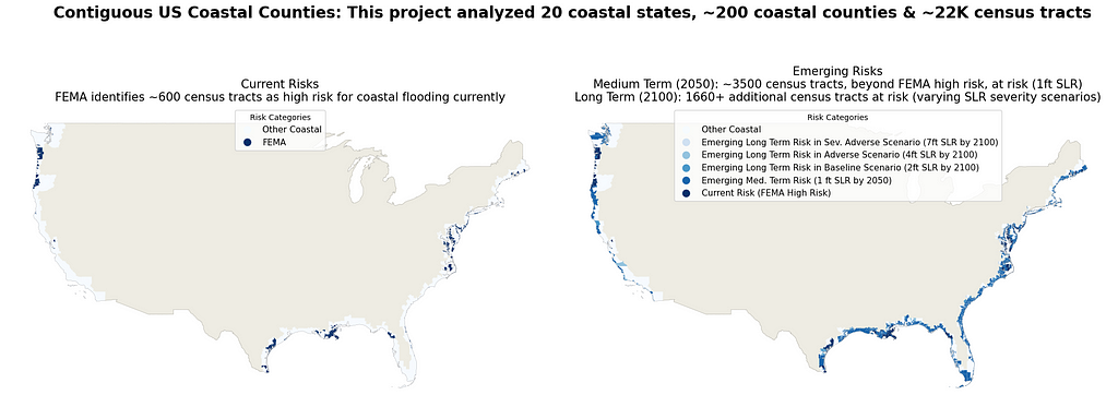
This project analyzed 20 coastal states in the contiguous United States covering ~200 coastal counties and ~22K coastal census tracts within them. Each census tract was analyzed in terms of whether is it currently known to be at risk, i.e., “Current Risk Regions”, vs. if it could be at risk in the future over the medium to long term, i.e., “Emerging Risk Regions”.
The first part of the project involved understanding current risks. In terms of sea level rise, one of the simplest forms in which it could manifest itself would be flooding. The Federal Emergency Management Agency (FEMA) has identified regions that are at high risk for flooding (FEMA floodplains)⁵ . This project used FEMA high risk floodplains as a proxy for areas that are currently known to be at risk for coastal flooding. In this project, these regions are considered “Current Risk Regions”.
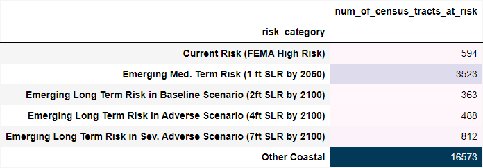
The second part of this project delved into identifying census tracts that may be at risk over the medium or longer term. This project leveraged sea level rise information from NOAA to identify census tracts that could become an emerging risk over the medium term (2050) or longer term (2100), i.e., “Emerging Risk Regions”. In order to better understand the severity of risk of rising sea leveles, emerging risk was divided into four categories — one category covering the medium term* and three scenario based longer term categores:
*as given there is more confidence in the SLR predictions, no scenario based approach is needed over the medium term.
The key observations through this analysis were that that outside of current FEMA high risk areas, there are ~3500 other census tracts along the contiguous US coastline that are expected to experience an average SLR increase of 1ft in the medium term (by 2050) and longer term (by 2100) an additional ~1660 census tracts are at risk for 2–7ft of SLR.
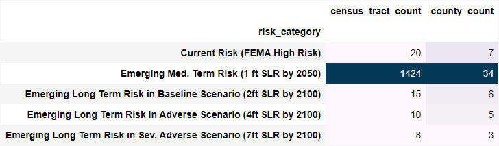
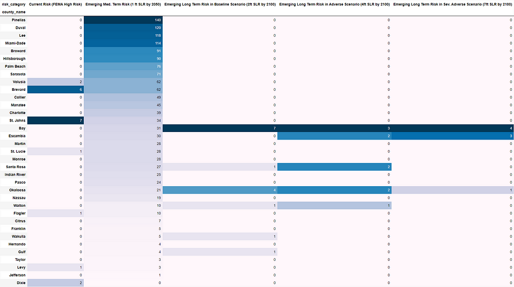
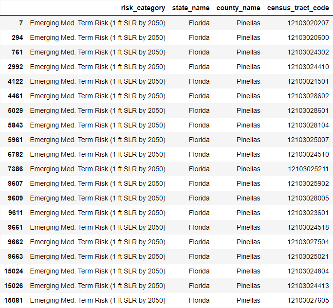
Presently, we know of 7 counties and 20 census tracts in Florida that are at high risk for flooding. However, in the future, multiple additional counties and census tracts are expected to be at risk for SLR, particularly in the medium term as shown below. Over the medium term (2050), 1424 additional census tracts will be at risk for SLR of 1ft. Over the longer term (2100), 33 additional census tracts may be at risk depending on the specific SLR scenario.
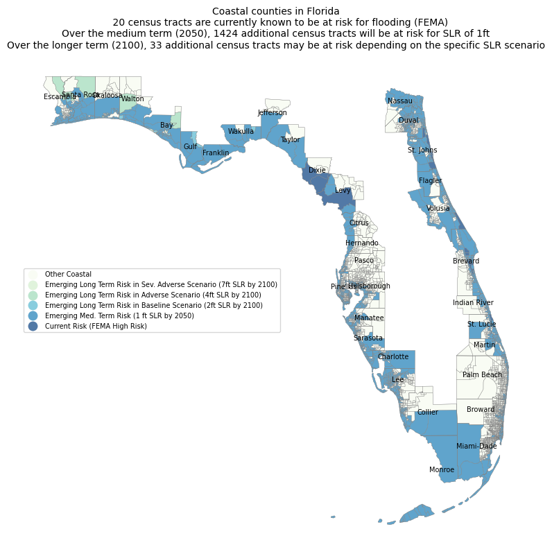
Note: similar analysis for other coastal states can be found in the appendices here
This project was implemented primarily in Jupyter Notebook using geopandas, as well as other standard Python libraries like pandas, matplotlib, seaborn, etc. The following datasets were utilied in the analysis needed for this project:
1. US Coastal Counties Population
3. NOAA 2022 Sea Level Rise Technical Report
4. Federal Reserve Board Stress Tests
7. Geospatial datafiles for contiguous US
9. FEMA National Risk Index (NRI)
Impact of Rising Sea Levels on Coastal Residential Real Estate Assets was originally published in Towards Data Science on Medium, where people are continuing the conversation by highlighting and responding to this story.
Originally appeared here:
Impact of Rising Sea Levels on Coastal Residential Real Estate Assets
Go Here to Read this Fast! Impact of Rising Sea Levels on Coastal Residential Real Estate Assets


Apple Silicon has brought impressive performance gains with great power efficiency. Can we use these chips for Deep Learning as well?
Originally appeared here:
3 ways to leverage Apple Silicon’s GPU for Deep Learning
Go Here to Read this Fast! 3 ways to leverage Apple Silicon’s GPU for Deep Learning

Uncovering Patterns in My Posts and Engagement — A data related one-year journey
Originally appeared here:
Exploring My LinkedIn Journey Through Data Analysis
Go Here to Read this Fast! Exploring My LinkedIn Journey Through Data Analysis

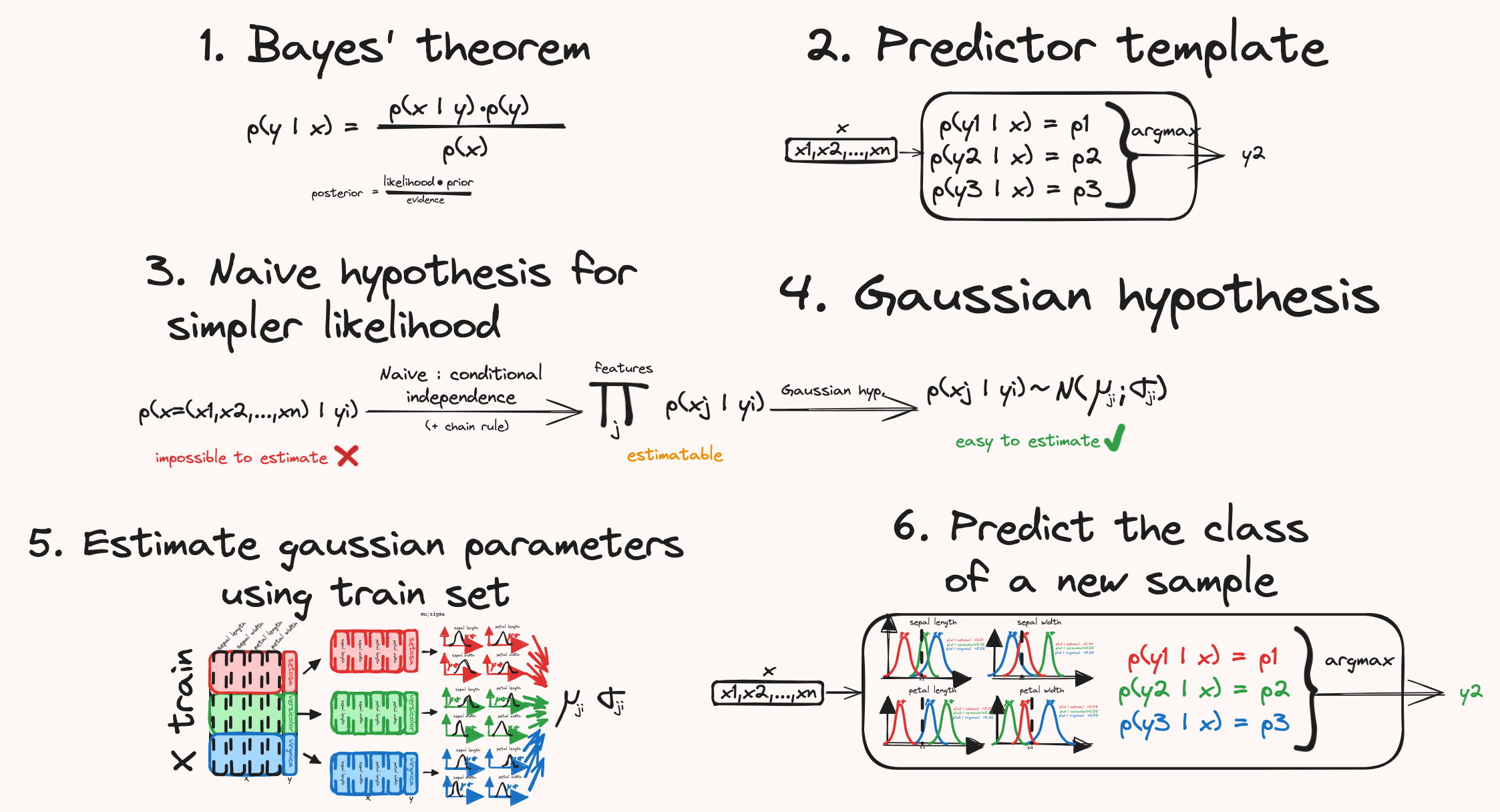
Solving the iris dataset with a gaussian approach in scikit-learn.
Originally appeared here:
Naive Bayes clearly explained