A way to program and tune prompt-agnostic LLM agent pipelines
I hate prompt engineering. For one thing, I do not want to prostrate before a LLM (“you are the world’s best copywriter … “), bribe it (“I will tip you $10 if you …”), or nag it (“Make sure to …”). For another, prompts are brittle — small changes to prompts can cause major changes to the output. This makes it hard to develop repeatable functionality using LLMs.
Unfortunately, developing LLM-based applications today involves tuning and tweaking prompts. Moving from writing code in a programming language that the computer follows precisely to writing ambiguous natural language instructions that are imperfectly followed does not seem like progress. That’s why I found working with LLMs a frustrating exercise — I prefer writing and debugging computer programs that I can actually reason about.
What if, though, you can program on top of LLMs using a high-level programming framework, and let the framework write and tune prompts for you? Would be great, wouldn’t it? This — the ability to build agent pipelines programmatically without dealing with prompts and to tune these pipelines in a data-driven and LLM-agnostic way — is the key premise behind DSPy.
An AI Assistant
To illustrate how DSPy works, I’ll build an AI assistant.
What’s an AI assistant? It’s a computer program that provides assistance to a human doing a task. The ideal AI assistant works proactively on behalf of the user (a chatbot can be a failsafe for functionality that is not easy to find in your product or a way end-users can reach out for customer support, but should not be the main/only AI assistance in your application). So, designing an AI assistant consists of thinking through a workflow and determining how you could want to streamline it using AI.
A typical AI assistant streamlines a workflow by (1) retrieving information such as company policies relevant to the task, (2) extracting information from documents such as those sent in by customers, (3) filling out forms or checklists based on textual analysis of the policies and documents, (4) collecting parameters and making function calls on the human’s behalf, and (5) identifying potential errors and highlighting risks.
The use case I will use to illustrate an AI assistant involves the card game bridge. Even though I’m building an AI assistant for bridge bidding, you don’t need to understand bridge to understand the concepts here. The reason I chose bridge is that there is a lot of jargon, quite a bit of human judgement involved, and several external tools that an advisor can use. These are the key characteristics of the industry problems and backoffice processes that you might want to build AI assistants for. But because it’s a game, there is no confidential information involved.
Agent Framework
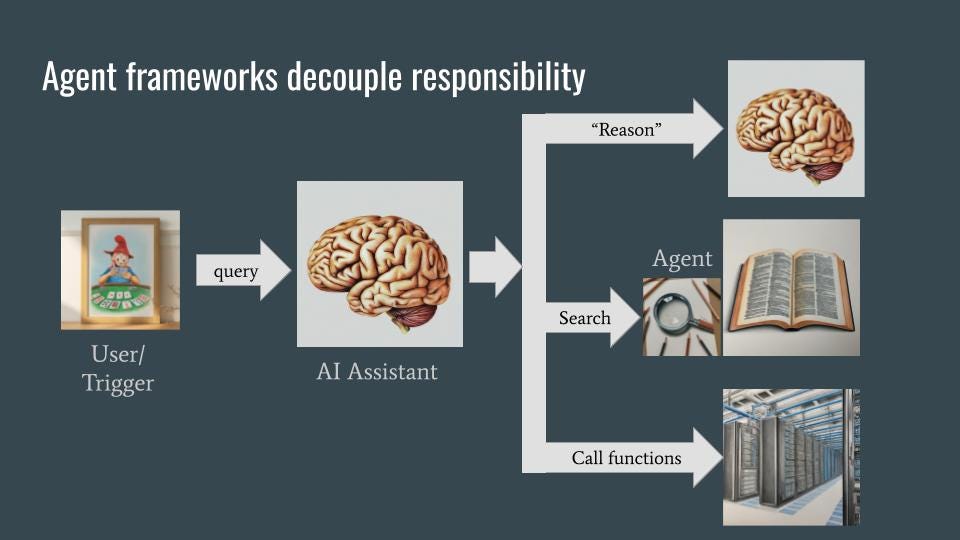
The assistant, when asked a question like “What is Stayman?”, uses a number of backend services to carry out its task. These backend services are invoked via agents, which are themselves built using language models. As with microservices in software engineering, the use of agents and backend services allows for decoupling and specialization — the AI assistant does not need to know how things are done, only what it needs done and each agent can know how to do only its own thing.
An agent framework. Image by author. Sketches in the image were generated using Gemini.
In an agent framework, the agents can often be smaller language models (LMs) that need to be accurate, but don’t have world knowledge. The agents will be able to “reason” (through chain-of-thought), search (through Retrieval-Augmented-Generation), and do non-textual work (by extracting the parameters to pass into a backend function). Instead of having disparate capabilities or skills, the entire agent framework is fronted by an AI assistant that is an extremely fluent and coherent LLM. This LLM will know the intents it needs to handle and how to route those intents. It needs to have world knowledge as well. Often, there is a separate policy or guardrails LLM that acts as a filter. The AI assistant is invoked when the user makes a query (the chatbot use case) or when there is a triggering event (the proactive assistant use case).
In DSPy, the process of sending a prompt to an LLM and getting a response back looks like this:
class ZeroShot(dspy.Module):
    """
    Provide answer to question
    """
    def __init__(self):
        super().__init__()
        self.prog = dspy.Predict("question -> answer")

    def forward(self, question):
        return self.prog(question="In the game of bridge, " + question)
There are four things happening in the snippet above:
Write a subclass of dspy.Module
In the init method, set up a LM module. The simplest is dspy.Predict which is a single call.
The Predict constructor takes a signature. Here, I say that there is one input (question) and one output (answer).
Write a forward() method that takes the input(s) specified (here: question) and returns the what was promised in the signature (here: answer). It does this by calling the dspy.Predict object created in the init method.
I could have just passed the question along as-is, but just to show you that I can somewhat affect the prompt, I added a bit of context.
Note that the code above is completely LLM-agnostic, and there is no groveling, bribery, etc. in the prompt.
To call the above module, you first initialize dspy with an LLM:
module = ZeroShot()
response = module("What is Stayman?")
print(response)
When I did that, I got:
Prediction(
    answer='Question: In the game of bridge, What is Stayman?nAnswer: A conventional bid of 2♣ by responder after a 1NT opening bid, asking opener to bid a four-card major suit if he has one, or to pass if he does not.'
)
Want to use a different LLM? Change the settings configuration lines to:
If all DSPy were doing was making it easier to call out to LLMs and abstract out the LLM, people wouldn’t be this excited about DSPy. Let’s continue to build out the AI assistant and tour some of the other advantages as we go along.
Let’s say that we want to use an LLM to do some entity extraction. We can do this by instructing the LLM to identify the thing we want to extract (date, product SKU, etc.). Here, we’ll ask it to find bridge jargon:
class Terms(dspy.Signature):
    """
    List of extracted entities
    """
    prompt = dspy.InputField()
    terms = dspy.OutputField(format=list)


class FindTerms(dspy.Module):
    """
    Extract bridge terms from a question
    """
    def __init__(self):
        super().__init__()
        self.entity_extractor = dspy.Predict(Terms)

    def forward(self, question):
        max_num_terms = max(1, len(question.split())//4)
        instruction = f"Identify up to {max_num_terms} terms in the following question that are jargon in the card game bridge."
        prediction = self.entity_extractor(
            prompt=f"{instruction}n{question}"
        )
        return prediction.terms
While we could have represented the signature of the module as “prompt -> terms”, we can also represent the signature as a Python class.
Calling this module on a statement:
module = FindTerms()
response = module("Playing Stayman and Transfers, what do you bid with 5-4 in the majors?")
print(response)
We’ll get:
['Stayman', 'Transfers']
Note how concise and readable this is.
RAG
DSPy comes built-in with several retrievers. But these essentially just functions and you can wrap existing retrieval code into a dspy.Retriever. It supports several of the more popular ones, including ChromaDB:
Of course, I had to get a document on bridge bidding, chunk it, and load it into ChromaDB. That code is in the repo if you are interested, but I’ll omit it as it’s not relevant to this article.
Orchestration
So now you have all the agents implemented, each as its own dspy.Module. Now, to build the orchestrator LLM, the one that receives the command or trigger and invokes the agent modules in some fashion.
Orchestration of the modules also happens in a dspy.Module:
class AdvisorSignature(dspy.Signature):
    definitions = dspy.InputField(format=str)  # function to call on input to make it a string
    bidding_system = dspy.InputField(format=str) # function to call on input to make it a string
    question = dspy.InputField()
    answer = dspy.OutputField()

class BridgeBiddingAdvisor(dspy.Module):
    """
    Functions as the orchestrator. All questions are sent to this module.
    """
    def __init__(self):
        super().__init__()
        self.find_terms = FindTerms()
        self.definitions = Definitions()
        self.prog = dspy.ChainOfThought(AdvisorSignature, n=3)

    def forward(self, question):
        terms = self.find_terms(question)
        definitions = [self.definitions(term) for term in terms]
        bidding_system = bidding_rag(question)
        prediction = self.prog(definitions=definitions,
                               bidding_system=bidding_system,
                               question="In the game of bridge, " + question,
                               max_tokens=-1024)
        return prediction.answer
Instead of using dspy.Predict for the final step, I’ve used a ChainOfThought (COT=3).
Optimizer
Now that we have the entire chain all set up, we can of course, simply call the orchestrator module to test it out. But more important, we can have dspy automatically tune the prompts for us based on example data.
To load in these examples and ask dspy to tune it (this is called a teleprompter, but the name will be changed to Optimizer, a much more descriptive name for what it does), I do:
traindata = json.load(open("trainingdata.json", "r"))['examples'] trainset = [dspy.Example(question=e['question'], answer=e['answer']) for e in traindata]
# use optimized advisor just like the original orchestrator response = optimized_advisor("What is Stayman?") print(response)
I used just 3 examples in the example above, but obviously, you’d use hundreds or thousands of examples to get a properly tuned set of prompts. Worth noting is that the tuning is done over the entire pipeline; you don’t have to mess around with the modules one by one.
Is the optimized pipeline better?
While the original pipeline returned the following for this question (intermediate outputs are also shown, and Two spades is wrong):
a: Playing Stayman and Transfers, what do you bid with 5-4 in the majors?
b: ['Stayman', 'Transfers']
c: ['Stayman convention | Stayman is a bidding convention in the card game contract bridge. It is used by a partnership to find a 4-4 or 5-3 trump fit in a major suit after making a one notrump (1NT) opening bid and it has been adapted for use after a 2NT opening, a 1NT overcall, and many other natural notrump bids.', "Jacoby transfer | The Jacoby transfer, or simply transfers, in the card game contract bridge, is a convention initiated by responder following partner's notrump opening bid that forces opener to rebid in the suit ranked just above that bid by responder. For example, a response in diamonds forces a rebid in hearts and a response in hearts forces a rebid in spades. Transfers are used to show a weak hand with a long major suit, and to ensure that opener declare the hand if the final contract is in the suit transferred to, preventing the opponents from seeing the cards of the stronger hand."]
d: ['stayman ( possibly a weak ... 1602', '( scrambling for a two -  ... 1601', '( i ) two hearts is weak  ... 1596']
Two spades.
The optimized pipeline returns the correct answer of “Smolen”:
a: Playing Stayman and Transfers, what do you bid with 5-4 in the majors?
b: ['Stayman', 'Transfers']
c: ['Stayman convention | Stayman is a bidding convention in the card game contract bridge. It is used by a partnership to find a 4-4 or 5-3 trump fit in a major suit after making a one notrump (1NT) opening bid and it has been adapted for use after a 2NT opening, a 1NT overcall, and many other natural notrump bids.', "Jacoby transfer | The Jacoby transfer, or simply transfers, in the card game contract bridge, is a convention initiated by responder following partner's notrump opening bid that forces opener to rebid in the suit ranked just above that bid by responder. For example, a response in diamonds forces a rebid in hearts and a response in hearts forces a rebid in spades. Transfers are used to show a weak hand with a long major suit, and to ensure that opener declare the hand if the final contract is in the suit transferred to, preventing the opponents from seeing the cards of the stronger hand."]
d: ['stayman ( possibly a weak ... 1602', '( scrambling for a two -  ... 1601', '( i ) two hearts is weak  ... 1596']
After a 1NT opening, Smolen allows responder to show 5-4 in the majors with game-forcing values.
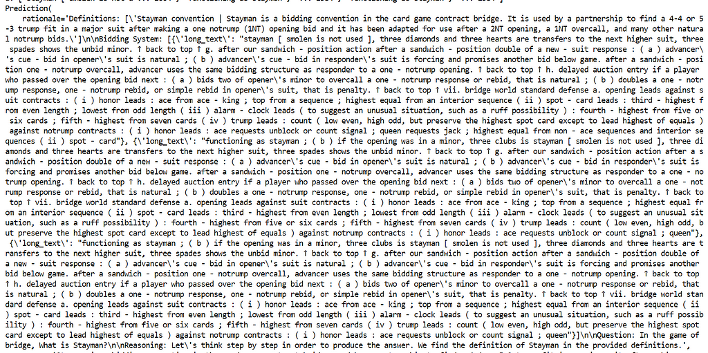
The reason is the prompt that dspy has created. For the question “What is Stayman?”, for example, note that it has built a rationale out of the term definitions, and several matches in the RAG:
Prompt created by dspy.ChainOfThought based on the term definitions, RAG, etc.
Again, I didn’t write any of the tuned prompt above. It was all written for me. You can also see where this is headed in the future— you might be able to fine-tune the entire pipeline to run on a smaller LLM.
A few months ago, Apple quietly released the first public version of its MLX framework, which fills a space in between PyTorch, NumPy and Jax, but optimized for Apple Silicon. Much like those libraries, MLX is a Python-fronted API whose underlying operations are largely implemented in C++.
Below are some observations of the similarities and differences between MLX and PyTorch. I implemented a bespoke convolutional neural network using PyTorch and its Apple Silicon GPU hardware support, and tested it on a few different datasets. In particular, the MNIST dataset, and the CIFAR-10 and CIFAR-100 datasets.
I implemented the model with PyTorch first, since I’m more familiar with the framework. The model has a series of convolutional and pooling layers, followed by a few linear layers with dropout.
This architecture is overkill for MNIST dataset classification, but I wanted something with some complexity to compare the two frameworks. I tested this against the CIFAR datasets, which approached around 40% accuracy; not amazing, but I suppose decent for something that isn’t a ResNet.
After finishing this implementation, I wrote a parallel implementation leveraging MLX. I happily discovered that most of the PyTorch implementation could be directly re-used, after importing the necessary MLX modules and replacing the PyTorch ones.
For example, the MLX version of the above code is here; it’s identical aside from a couple of differences in named parameters.
Notes on MLX
MLX has some interesting properties worth calling out.
Array
MLX’s array class takes the place of Tensor; much of the documentation compares it to NumPy’s ndarray, however it is also the datatype used and returned by the various neural network layers available in the framework.
array works mostly as you’d expect, though I did have a bit of trouble converting back and forth between deeply-nested np.ndarrays and mlx.arrays necessitating some list type shuffling to make things work.
Lazy Computation
Operations in MLX are lazily evaluated; meaning that the only computation executed in the lazily-built compute graph is that which generates outputs actually used by the program.
There are two ways to force evaluation of the results of operations (such as inference):
Calling mlx.eval() on the output
Referencing the value of a variable for any reason; for example when logging or within conditional statements
This can be a little tricky when trying to manage the performance of the code, since a reference (even an incidental one) to any value triggers an evaluation of that variable as well as all intermediate variables within the graph. For example:
def classify(X, y): model = MyModel() # Not yet initialized p = model(X) # Not yet computed loss = mlx.nn.losses.nll_loss(p, y) # Not yet computed
# Without the print() above, would return `p` and lazy `loss` return p, loss
This behavior also makes a little difficult to build one-to-one benchmarks between PyTorch and MLX-based models. Since training loops may not evaluate outputs within the loop itself, its computation needs to be forced in order to track the time of the actual operations.
test_start = time.perf_counter_ns() # Start time block
accuracy, _ = eval(test_data_loader, model, n)
mx.eval(accuracy) # Force calculation within measurement block
test_end = time.perf_counter_ns() # End time block
There’s a tradeoff between accumulating a large implicit computation graph, and regularly forcing the evaluation of that graph during training. For example, I was able to lazily run through all of this model’s training epochs over the dataset in just a few seconds. However, the eventual evaluation of that (presumably enormous) implicit graph took roughly the same amount of time as eval’ing after each batch. This is probably not always the case.
Compilation
MLX provides the ability to optimize the execution of pure functions through compilation. These can be either a direct call to mlx.compile() or an annotation (@mlx.compile) on a pure function (without side effects).
There are a few gotchas related to state mutation when using compiled functions; these are discussed in the docs.
As mentioned above, it was pretty easy to convert much of my PyTorch code into MLX-based equivalents. A few differences though:
Some of the neural network layers discretely expect different configurations of inputs. For example, mlx.nn.Conv2d expects input images in NHWC format (with C representing the channels dimensionality), while torch.nn.Conv2d expects NCHW ; there are a few other examples of this. This required some conditional tensor/array shuffling.
Model implementations, deriving from nn.Module, aren’t expected to override forward() but rather __call__() for inference
I assume because of the potential for function compilation, as well as the lazy evaluation support mentioned above, the process of training using MLX optimizers is a bit different than with a typical PyTorch model. Working with the latter, one is used to the standard format of something like:
for X, y in dataloader:
  p = model(X)
  loss = loss_fn(p, y)
  optimizer.zero_grad()
  loss.backward()
  optimizer.step()
# batch_iterate is a custom generator function for X, y in batch_iterate(batch_size, train_images, train_labels): loss = step(X, y)
Which is fine, but a bit more involved than I was expecting. Otherwise, everything felt very familiar.
Performance
Note that all results below are from my MacBook Air M2.
This CNN has three configurations: PyTorch CPU, PyTorch GPU, and MLX GPU. As a sanity check, over 30 epochs, here’s how the three compare in terms of accuracy and loss:
Accuracy and Loss over 30 epochs; visualization code available in the linked repository
The results here are all in the same ballpark, though it’s interesting that the MLX-based model appears to converge more quickly than the PyTorch-based ones.
In addition, it seems like the accuracy of the MLX model is consistently slightly below that of the PyTorch-based models. I’m not sure what accounts for that discrepancy.
In terms of runtime performance, I had other interesting results:
Training epoch runtime variance across the three model configurations
When training the model, the PyTorch-based model on the CPU unsurprisingly took the most time, from a minimum of 36 to a maximum of 45 seconds per epoch. The MLX-based model, running on the GPU, had a range of about 21–27 seconds per epoch. PyTorch running on the GPU, via the MPS device , was the clear winner in this regard, with epochs ranging from 10–14 seconds.
Classification over the test dataset of ten thousand images tells a different story.
Total time taken by each model variant to classify all 10k images in the test dataset; batches of 512
While it took the CPU-based model around 1700ms to classify all 10k images in batches of 512, the GPU-based models completed this task in 1100ms for MLX and 850ms for PyTorch.
However, when classifying the images individually rather than in batches:
Total time taken by each model variant to classify all 10k images in the test dataset; single images at a time over ten thousand.
Apple Silicon uses a unified memory model, which means that when setting the data and model GPU device to mps in PyTorch via something like .to(torch.device(“mps”)) , there is no actual movement of data to physical GPU-specific memory. So it seems like the overhead associated with PyTorch’s initialization of Apple Silicon GPUs for code execution is fairly heavy. As seen further above, it works great during parallel batch workloads. But for individual record classification after training, it was far outperformed by whatever MLX is doing under the hood to spin up GPU execution more quickly.
Profiling
Taking a quick look at some cProfile output for the MLX-based model, ordered by cumulative execution time:
We some time spent here in a few layer functions, with the bulk of time spent in mlx.core.eval(), which makes sense since it’s at this point in the graph that things are actually being computed.
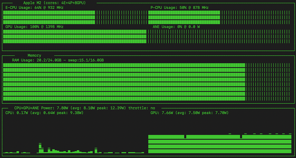
Using asitop to visualize the underlying timeseries powertools data from MacOS:
Interestingly, the top function appears to be Tensor.item(), which is called in various places in the code to calculate loss and accuracy, and possibly also within some of the layers referenced lower in the stack. Removing the tracking of loss and accuracy during training would probably have a noticeable improvement on overall training performance.
asitop power history — PyTorch GPU model run
Compared to the MLX model, the PyTorch variant doesn’t seem to have saturated the GPU during training (I didn’t see it breach 95%), and has a higher balance of usage on the CPU’s E cores and P cores.
It’s interesting that the MLX model makes heavier use of the GPU, but trains considerably more slowly.
Neither model (CPU or GPU-based) appears to have engaged the ANE (Apple Neural Engine).
Final Thoughts
MLX was easy to pick up, and that should be the case for anyone with experience using PyTorch and NumPy. Though some of the developer documentation is a bit thin, given the intent to provide tools compatible with those frameworks’ APIs, it’s easy enough to fill in any gaps with the corresponding PyTorch or NumPy docs (for example, SGD [1] [2]).
The overall performance of the MLX model was pretty good; I wasn’t sure whether I was expecting it to consistently outperform PyTorch’s mps device support, or not. While it seemed like training was considerably faster through PyTorch on the GPU, single-item prediction, particularly at scale, was much faster through MLX for this model. Whether that’s an effect of of my MLX configuration, or just the properties of the framework, its hard to say (and if its the former — feel free to leave an issue on GitHub!)
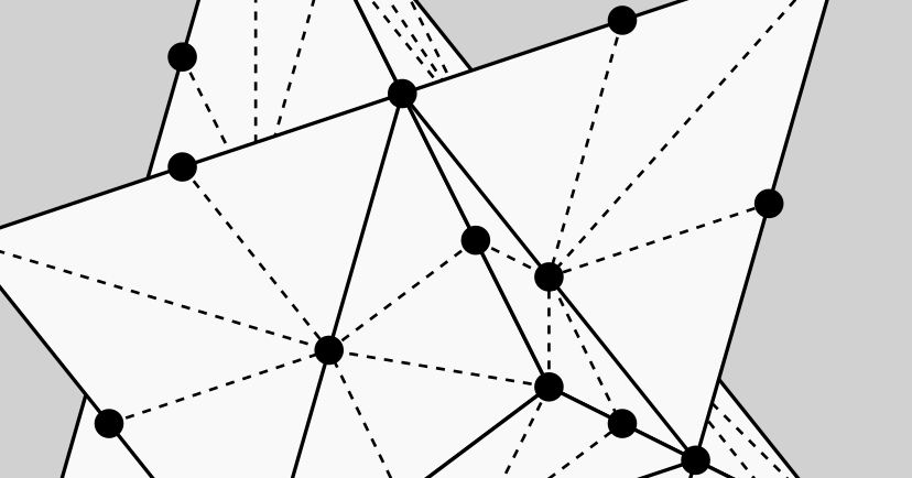
How 2D grid-based algorithms can be brought into the 3D world
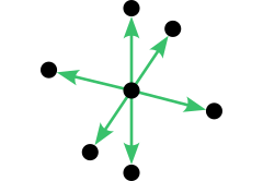
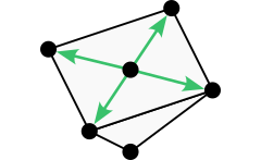
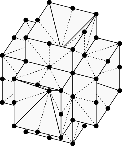
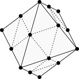
Closeup of the triangular 50-neighborhood. (Image by author)
In my previous two articles, A Short and Direct Walk with Pascal’s Triangle and A Quick and Clear Look at Grid-Based Visibility, we saw how easy it is to generate decent-looking travel paths and compute visible regions using grid-based algorithms. The techniques I shared in those posts can be used for video games, mobile robotics, and architectural design, though our examples were limited to two dimensions. In this third and final installment of the series, we take what we know about 2D grid-based algorithms and add the third dimension. Read on to discover five 3D grid neighborhoods you can use to solve AI problems like navigation and visibility in 3D.
3D Navigation and Visibility Problems
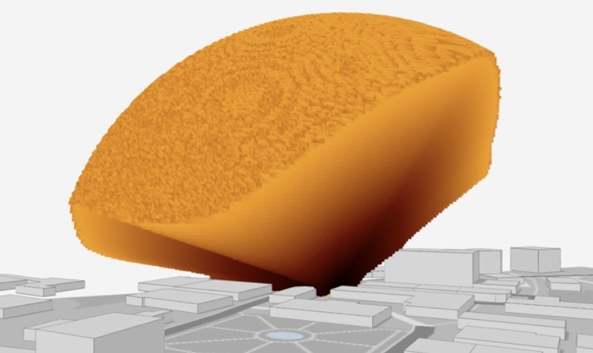
Since the world is 3D, it’s no surprise that video games, mobile robotics challenges, and architectural design tools often require 3D variants of pathfinding and visibility algorithms. For example, the image below shows what a person can see from a certain point in a 3D model of a city. An architect might use this kind of 3D visibility analysis to design a large building while allowing nearby pedestrians to see as much of the sky as possible.
The above example is typical of 3D pathfinding in that the path is constrained to walkable surfaces such as staircases and floors. Another type of 3D navigation problem arises when generating a flight path for an aerial robot such as a quadcopter drone. In that case, the path may go straight through the air instead of adhering to surfaces.
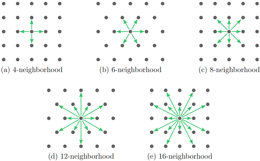
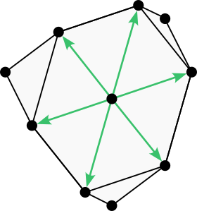
As in the previous articles, we are interested in solving navigation and visibility problems using grid-based algorithms. This means that every time a grid point is visited, information may flow only to neighboring grid points. The set of grid points considered to be “neighbors” is given by the grid neighborhood. There are many possible grid neighborhoods, but the ones depicted in the image below are the five smallest standard 2D grid neighborhoods [1]. Notice that as the neighborhoods increase in size from 4 to 16 neighbors, they alternate between rectangular and triangular grids. Generally speaking, algorithms that use larger neighborhoods take longer to run but produce more accurate results.
Rectangular and triangular 2D grid neighborhoods. (Image by Autodesk Research [1], used with permission)
What interests us now is the following question:
What do these 2D neighborhoods look like in 3D?
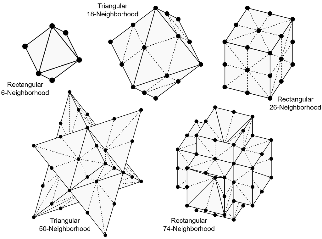
The 3D equivalent of the 4-neighborhood and the 8-neighborhood are described in the journal paper “Path Counting for Grid-Based Navigation” and elsewhere in the literature, but I had difficulty finding the 3D versions of the other three neighborhoods. I eventually decided to work them out myself so that I could present the complete set. Before we go through them one by one, here’s a sneak peek at the five smallest standard 3D grid neighborhoods.
The five smallest standard grid neighborhoods in 3D. (Image by author)
To demonstrate these five neighborhoods, we’ll solve the 3D visibility problem with each of them and compare the five solutions for accuracy. The reason we’re focusing on grid-based visibility is because it’s one of the simplest grid-based algorithms — simple enough for us to take a good look at the code. Once you’ve seen how grid-based visibility can be implemented in 3D, you can use your choice of 3D grid neighborhood to solve 3D pathfinding problems and other AI challenges that arise in the 3D world.
Rectangular 6-Neighborhood
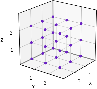
We’ll start with the neighborhoods defined on a 3D rectangular grid, which is simply the set of points [x, y, z] where x, y, and z are integers. These grids are widely used. They can be represented on a computer using a standard 3D array.
A 3x3x3 slice of a 3D rectangular grid. (Image by author)
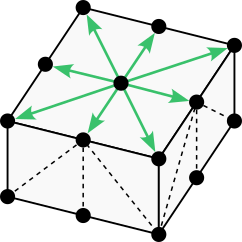
The first 3D grid neighborhood is nearly ubiquitous, but we’ll present it anyway for the sake of completeness. When the rectangular 4-neighborhood in 2D is extended to 3D, we end up with the rectangular 6-neighborhood illustrated below. To interpret the image, imagine that the two vertical arrows point up and down while the remaining arrows point north, east, south, and west.
The rectangular 6-neighborhood represented with vectors. (Image by author)
Now we’ll apply the rectangular 6-neighborhood to solve the 3D visibility problem using Python. In the code below, the function grid_visibility inputs a 3D array named grid0 representing the environment. Cells in this initial grid with a value of 1 represent empty space, and cells with a value of 0 represent an obstacle. The function computes the visibility results in a separate 3D array named grid. Cells in this output grid with a value of 1 are considered visible from a viewpoint at [0, 0, 0], and cells with a value of 0 are considered blocked.
import numpy as np

# Solve the 3D visibility problem using a simple grid-based method
def grid_visibility(grid0):
    grid = grid0.copy()
    for x in range(grid.shape[0]):
        for y in range(grid.shape[1]):
            for z in range(int(x==0 and y==0), grid.shape[2]):
                vx = grid[x-1,y,z]
                vy = grid[x,y-1,z]
                vz = grid[x,y,z-1]
                grid[x,y,z] *= (x*vx + y*vy + z*vz) / (x + y + z)
    return grid >= 0.5
The reason the viewpoint is fixed at [0, 0, 0] is just to simplify the code. If you want the viewpoint to be located somewhere else, such as the center of the grid, the previous article solves that problem in 2D with an array indexing trick that will also work in 3D.
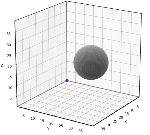
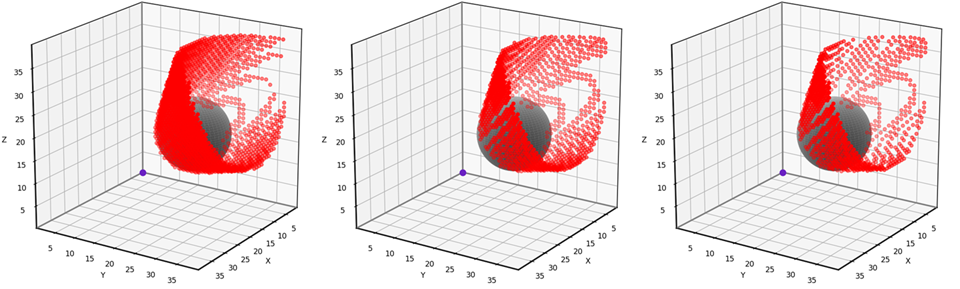
To test our 3D grid-based visibility solver, we’ll use the scenario shown below. The input grid is 40x40x40 and features a spherical obstacle with center at [10, 20, 16] and radius 8.
The test scenario. (Image by author)
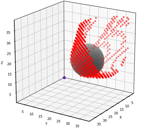
This problem is simple enough to solve analytically, allowing us to test the accuracy of the grid-based solution. The red dots in the animation below indicate the grid points that have been misclassified using our 6-neighbor grid-based approach. Notice that the vast majority of the 40x40x40 grid points have no red dot, meaning that they are correctly classified. The errors occur near the boundary of the obstacle’s “shadow”, where grid points are either barely visible or barely obstructed. I find that errors such as these are usually tolerable, though it depends on the application. I’ll provide the testing and visualization code near the end of the article.
Grid-based visibility classification errors using the 6-neighborhood. (Animation by author)
Now we are going to rewrite our grid-based visibility algorithm in a way that accommodates the larger 3D grid neighborhoods. The key is to solve the visibility problem within a cone bracketed by a set of vectors. In the previous article, we defined a 2D visibility_within_cone function that required two vectors to specify a triangular cone. In 3D, the function requires three vectors to define a tetrahedral cone.
# Solve the 3D visibility problem by modifying a grid within a cone
def visibility_within_cone(grid, u_vector, v_vector, w_vector):
    u = np.asarray(u_vector, dtype=int)
    v = np.asarray(v_vector, dtype=int)
    w = np.asarray(w_vector, dtype=int)
    origin = np.array([0,0,0], dtype=int)
    dims = np.asarray(grid.shape, dtype=int)
    m = 0
    k = 0
    q = 0
    pos = np.array([0,0,0], dtype=int)
    while np.all(pos < dims):
        while np.all(pos < dims):
            while np.all(pos < dims):
                if not np.all(pos == 0):
                    p = tuple(pos)
                    if grid[p] == 1:
                        pu = tuple(np.maximum(origin, pos - u))
                        pv = tuple(np.maximum(origin, pos - v))
                        pw = tuple(np.maximum(origin, pos - w))
                        grid[p] = (m*grid[pu] +
                                   k*grid[pv] +
                                   q*grid[pw]) / (m + k + q)
                q += 1
                pos += w
            k += 1
            q = 0
            pos = m*u + k*v
        m += 1
        k = 0
        q = 0
        pos = m*u
Below is an alternative illustration of the 6-neighborhood showing the triangular faces associated with each cone. Represented in this fashion, the 6-neighborhood appears as an octahedron.
The rectangular 6-neighborhood represented with triangular faces. (Image by author)
If we slice the octahedron in half, we can see the rectangular 6-neighborhood’s 2D counterpart: the 4-neighborhood.
The 3D 6-neighborhood cut in half to reveal the 2D 4-neighborhood. (Image by author)
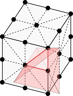
Let’s look at the full octahedron again, and project one of the triangles away from the origin to help us visualize a tetrahedral cone. The 6-neighborhood has 8 such cones in total, one for each 3D octant of the domain. Note that each cone extends to infinity, taking up its entire octant.
Visualization of a cone in the rectangular 6-neighborhood. (Image by author)
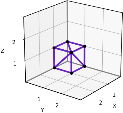
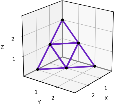
Here is a plot of just one octant of the 6-neighborhood, with its single cone. The plot makes it easy to read off the coordinates of the bracketing vectors, which we’ll need in order to reimplement the grid-based algorithm. In this case the bracketing vectors are [1,0,0], [0,1,0], [0,0,1], the corners of the triangle.
Plot of a cone in one octant of the rectangular 6-neighborhood. (Image by author)
Below is our new implementation of 6-neighbor 3D grid-based visibility.
# Solve the 3D visibility problem using the 6-neighborhood
def grid6_visibility(grid0):
    grid = grid0.copy()
    visibility_within_cone(grid, [1,0,0], [0,1,0], [0,0,1])
    return grid >= 0.5
The new grid6-visibility function produces exactly the same results as the grid-visibility function we saw earlier, but our refactoring efforts will help us tackle the larger 3D neighborhoods which have many more cones.
Rectangular 26-Neighborhood
When the rectangular 8-neighborhood in 2D is extended to 3D, we get the rectangular 26-neighborhood shown below. The neighborhood appears as a 2x2x2 cube with each side tessellated into triangles representing cones.
The rectangular 26-neighborhood. (Image by author)
As before, we can cut the neighborhood in half to see its 2D counterpart: the 8-neighborhood.
The 3D 26-neighborhood cut in half to reveal the 2D 8-neighborhood. (Image by author)
The rectangular 26-neighborhood is well known, though it is rarely shown in a way that identifies its 48 tetrahedral cones. The illustration below highlights one of these cones.
Visualization of a cone in the rectangular 26-neighborhood. (Image by author)
The following plot helps us to read off the coordinates of the 6 cones within one octant.
Plot of the 6 cones in one octant of the rectangular 26-neighborhood. (Image by author)
Here’s our implementation of 26-neighbor 3D grid-based visibility. Notice that we call visibility_within_cone once for each triangle in the plot above.
# Solve the 3D visibility problem using the 26-neighborhood
def grid26_visibility(grid0):
    grid = grid0.copy()
    visibility_within_cone(grid, [1,0,0], [1,1,0], [1,1,1])
    visibility_within_cone(grid, [1,0,0], [1,0,1], [1,1,1])
    visibility_within_cone(grid, [0,1,0], [1,1,0], [1,1,1])
    visibility_within_cone(grid, [0,1,0], [0,1,1], [1,1,1])
    visibility_within_cone(grid, [0,0,1], [1,0,1], [1,1,1])
    visibility_within_cone(grid, [0,0,1], [0,1,1], [1,1,1])
    return grid >= 0.5
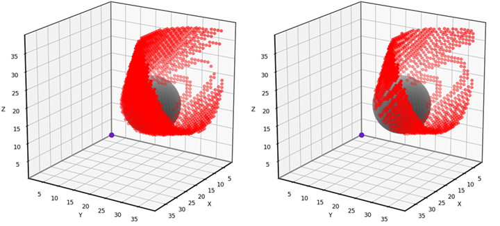
The visibility results we obtain with the 26-neighborhood contain fewer errors than with the 6-neighborhood. You can see below that the red dots are sparser.
Classification errors using the 6-neighborhood (left) and 26-neighborhood (right). (Image by author)
The 26-neighborhood is common, though it is usually presented without identifying the 48 tetrahedral cones. In theory these cones aren’t needed for pathfinding or visibility, but they allow us to adopt faster algorithms. For example, it is widely understood among computer scientists that one can find shortest grid paths in 3D by applying Dijkstra’s algorithm using 26 neighbors on a rectangular grid. Dijkstra’s algorithm does not require us to know how those neighbors are grouped into cones. However, if we have identified the cones, we can adopt a faster pathfinding method called 3D Jump Point Search [2]. If you’re looking for a challenge, try implementing Jump Point Search with your choice of 3D grid neighborhood.
Rectangular 74-Neighborhood
The previous two 3D grid neighborhoods are reasonably well established, but now we must venture into unknown territory. When the rectangular 16-neighborhood in 2D is extended to 3D, we get the rectangular 74-neighborhood. I’m not sure how to describe the shape of the 74-neighborhood, but this is what it looks like.
The rectangular 74-neighborhood. (Image by author)
And here it is again, this time sliced in half to reveal the 16-neighborhood.
The 3D 74-neighborhood cut in half to reveal the 2D 16-neighborhood. (Image by author)
The rectangular 74-neighborhood has 144 cones in total. Below is a plot representing the 18 cones in one octant.
Plot of the 18 cones in one octant of the rectangular 74-neighborhood. (Image by author)
Reading off the coordinates of each triangle in the plot, we can now implement 74-neighbor 3D grid-based visibility.
Below are the errors for all three of our 3D rectangular grid neighborhoods applied to the test scenario. The 74-neighbor solution contains the fewest misclassified points.
Classification errors using the 6-neighborhood (left), 26-neighborhood (center), and 74-neighborhood (right). (Image by author)
Triangular 18-Neighborhood
With the 3D rectangular neighborhoods taken care of, it’s time to see what the triangular neighborhoods look like in 3D. They’re surprisingly hard to visualize! A good way to start is by asking the following question:
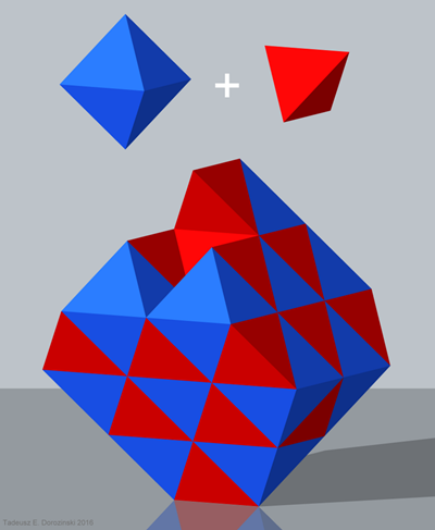
What solid objects have faces that are equilateral triangles, and can be used to fill 3D space?
Aristotle took a stab at answering that question over 2000 years ago. He famously taught that regular tetrahedra fill space [3]. He was wrong. If you have a whole bunch of regular tetrahedra and try putting them together, you will necessarily end up with gaps. The same can be said for regular octahedra: they also do not fill space. But as shown below, you can fill space using both tetrahedra and octahedra.
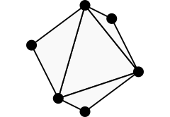
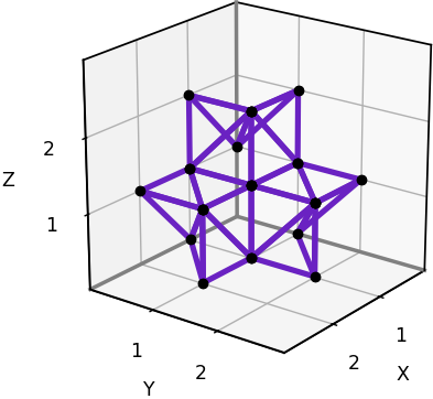
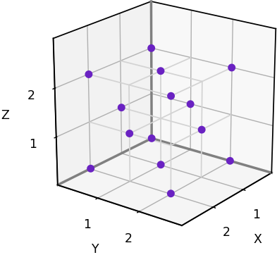
In the space-filling arrangement above, notice that the vertices of the tetrahedra and octahedra occur at regularly spaced points. These are the points of a face-centered cubic lattice, which we’ll refer to as a 3D triangular grid. If one of these points is located at [0, 0, 0], we can scale and orient the 3D triangular grid so that its points coincide with every alternate point on a 3D rectangular grid. The plot below shows a 3D triangular grid with this configuration.
A 3x3x3 slice of a 3D triangular grid. (Image by author)
To represent these grids on a computer, we’ll adopt the same kind of arrays that we employed for 3D rectangular grids. However, in the case of a 3D triangular grid, only half of the array elements will ever get used. An array element at [x, y, z] will be used only if (x + y + z) is an even number. If (x + y + z) is odd, the element will be initialized to 0 and will always remain 0.
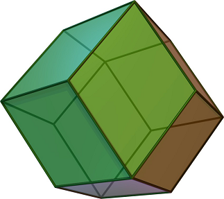
We now know how points in a 3D triangular grid can be arranged, but what does a triangular grid cell look like in 3D? When I use the term “grid cell”, I’m referring to a space filling shape that is centered on a grid point. In 2D, a triangular grid cell is not a triangle, but rather a hexagon. The Red Blog Games tutorial on Hexagonal Grids makes this easy to see. It turns out that in 3D, a triangular grid cell is called a rhombic dodecahedron. Rhombic dodecahedra fill 3D space.
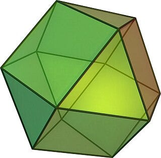
The dual of a polyhedron is the shape you get when you replace each face with a vertex and each vertex with a face. The dual of a rhombic dodecahedron is called a cuboctahedron.
If we center a cuboctahedron on a 3D triangular grid point, we can scale and orient it so that its 12 vertices coincide with the nearest neighboring grid points. In other words, the cuboctahedron is a viable 3D grid neighborhood. I would not consider this 12-neighborhood to be a standard 3D grid neighborhood, however, for the simple reason that some its faces are squares rather than triangles. There is a grid-based visibility algorithm from the urban design community that could be adapted to work with the square faces of the 12-neighborhood [4], but we will stick with our current algorithm requiring triangular faces.
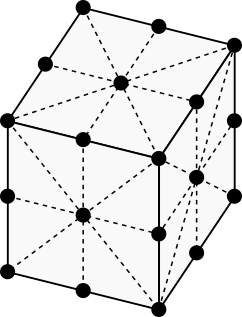
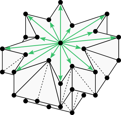
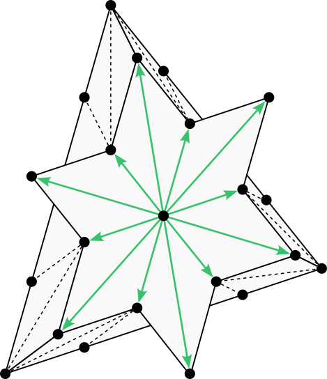
The smallest 3D triangular neighborhood that meets our criteria is the triangular 18-neighborhood. It appears as an octahedron with each side tessellated into triangles.
The triangular 18-neighborhood. (Image by author)
If we slice the 18-neighborhood at an angle, we can see that it extends the 2D triangular 6-neighborhood.
The 3D 18-neighborhood cut in half to reveal the 2D 6-neighborhood. (Image by author)
The triangular 18-neighborhood has 32 cones, 4 cones per octant.
Plot of the 4 cones in one octant of the triangular 18-neighborhood. (Image by author)
Here’s our 18-neighbor implementation of grid-based visibility.
# Solve the 3D visibility problem using the 18-neighborhood
def grid18_visibility(grid0):
    grid = grid0.copy()
    visibility_within_cone(grid, [2,0,0], [1,1,0], [1,0,1])
    visibility_within_cone(grid, [0,2,0], [1,1,0], [0,1,1])
    visibility_within_cone(grid, [0,0,2], [1,0,1], [0,1,1])
    visibility_within_cone(grid, [1,1,0], [1,0,1], [0,1,1])
    return grid >= 0.5
And here are the results.
Classification errors using the 18-neighborhood. (Image by author)
At first glance it may seem that the 18-neighborhood has yielded greater accuracy than the three rectangular neighborhoods, even the ones with more neighbors and cones. However, the main reason the red dots are sparser here than in previous plots is because, for 3D triangular grids, we only evaluate every alternate point [x, y, z].
Triangular 50-Neighborhood
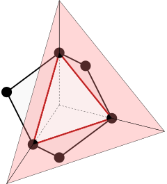
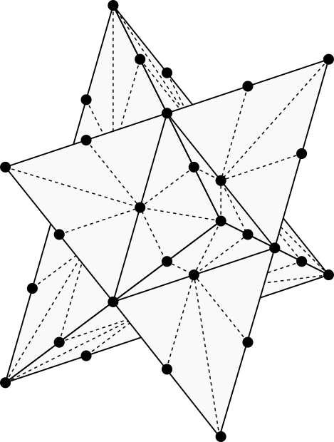
The fifth and final neighborhood in our collection is the triangular 50-neighborhood. Its overall shape is known as a stellated octahedron, which is basically an octahedron with a tetrahedron glued onto each face. In the case of the 50-neighborhood, each face of the stellated octahedron is tessellated into 4 triangles, as shown below.
The triangular 50-neighborhood. (Image by author)
The 50-neighborhood extends the 2D triangular 12-neighborhood.
The 3D 50-neighborhood cut in half to reveal the 2D 12-neighborhood. (Image by author)
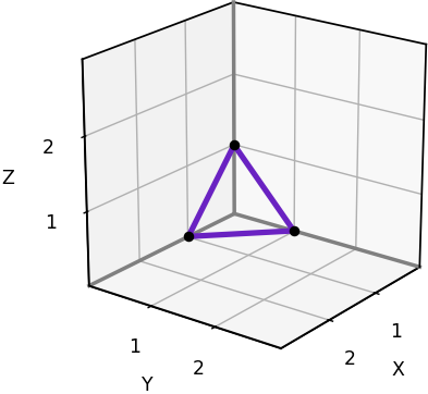
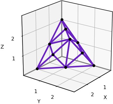
It has 96 cones, 12 per octant.
Plot of the 12 cones in one octant of the triangular 50-neighborhood. (Image by author)
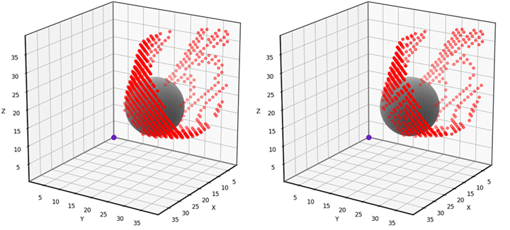
And finally, here are the results for both of our 3D triangular grid neighborhoods. It may be hard to tell at a glance, but the 50-neighbor results contain fewer errors.
Classification errors using the 18-neighborhood (left) and 50-neighborhood (right). (Image by author)
Comparison of Neighborhoods
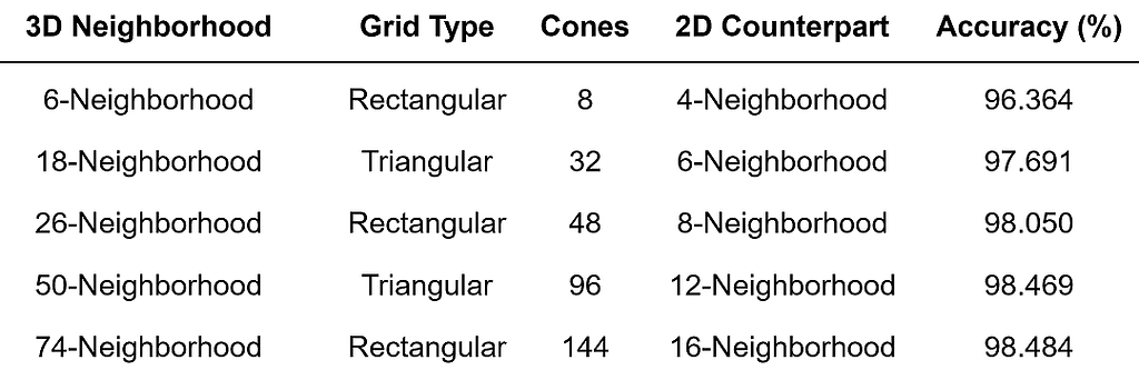
The table below lists the five presented 3D grid neighborhoods, their properties, and the accuracy obtained when applying each neighborhood to our test problem. The accuracy values are calculated by taking the number of grid points correctly classified as visible or not visible, and dividing by the total number of evaluated grid points. As we’d expect, the accuracy scores increase with the number of neighbors.
List of 3D grid neighborhoods, their properties, and accuracy results. (Image by author)
This analysis is mostly for illustrative purposes. If our goal were to perform a rigorous comparison of these five 3D grid neighborhoods, we would not be satisfied with our single test scenario. Instead we would want to apply each neighborhood to a large set of test scenarios, and average the results.
I should also point out that in this article and the previous one, I have taken a shortcut both literally and figuratively when implementing grid-based visibility for large neighborhoods. The proper formula, which you can find in the journal paper “Path Counting for Grid-Based Navigation” [1], requires a line-of-sight test between every pair of neighboring grid points. To illustrate, consider the following 2D scenario.
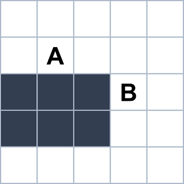
Two labelled cells on a 2D rectangular grid. (Image by author)
If we’re using the 4-neighborhood or the 8-neighborhood, then cells A and B in the above example are not neighbors. But if we’re using the 16-neighborhood, then these two points are neighbors and so we should technically perform a line-of-sight test between them. The algorithms in this article series alleviate the need for line-of-sight checks between distant grid points, though it is still best to precompute these checks over the short distances between neighbors. If we draw a line between the centers of cells A and B, the line will pass through a blocked cell. This suggests that the visibility algorithm should probably not propagate information directly from A to B.
The literal and figurative shortcut I’ve been taking is to assume two neighboring cells are mutually visible as long as they’re both empty. This works perfectly well for the 4-neighborhood in 2D and the 6-neighborhood in 3D, but it isn’t quite right for the larger neighborhoods. In the example above, a 16-neighbor version of my Python code would treat cells A and B as mutually visible. It would happily propagate information from one to the other, essentially taking a “shortcut” through the obstacle.
This shortcut I’m describing isn’t such a big deal if our obstacles are sufficiently wide compared with the grid spacing. In our test results, the larger 3D neighborhoods achieved greater accuracy than the smaller ones despite this flaw. But if you plan to use large 2D or 3D grid neighborhoods in your own work, I encourage you to carefully consider which neighboring grid points should and should not be treated as direct pathways for information.
Testing and Visualization Code
Please skip this section and proceed to the conclusion if you are not interested in running the Python code presented in this article.
If you are interested in running the code, follow these steps:
Make sure you have Python installed along with the NumPy and Matplotlib libraries.
Create an empty text file named grid_visibility_3D.py. Starting from the top, copy into this text file all of the code blocks that have appeared in this article until this point.
Create another text file named test_grid_visibility_3D.py and copy in the long code block that appears below these instructions.
On the command prompt, run python test_grid_visibility_3D.py. You should see the same accuracy scores that were reported in the Comparison of Neighborhoods table. You should also see a 3D visualization of the test scenario.
Close the visualization window and run the command python test_grid_visibility_3D.py 6. You should see the same output except with red dots appearing in the 3D visualization. You can drag the cursor on the plot to rotate it and get a better view. These dots are the errors associated with the 6-neighbor visibility algorithm. Run the code again with the command line argument 6 changed to 18, 26, 50, or 74 to see the errors associated with the other 3D grid neighborhoods.
from grid_visibility_3D import *
import matplotlib.pyplot as plt import sys
# Set dimensions for the test scenario nx = 40 ny = 40 nz = 40
# Set spherical obstacle parameters for the test scenario x_sphere = 10 y_sphere = 20 z_sphere = 16 r_sphere = 8
# Initialize the 3D visibility problem for the test scenario def initial_grid(): grid = np.ones((nx,ny,nz)) p_sphere = np.array([x_sphere, y_sphere, z_sphere]) for x in range(nx): for y in range(ny): for z in range(nz): p = np.array([x,y,z]) r = np.sqrt(np.sum((p - p_sphere)**2)) if r < r_sphere: grid[x,y,z] = 0 return grid
# Solve the 3D visibility problem analytically for the test scenario def analytic_solution(): grid = initial_grid() p_sphere = np.array([x_sphere, y_sphere, z_sphere]) d_sphere = np.sqrt(np.sum(p_sphere**2)) u = p_sphere/d_sphere for x in range(nx): for y in range(ny): for z in range(nz): if grid[x,y,z]: p = np.array([x,y,z]) d = np.sum(p*u) if d > d_sphere: h = np.sqrt(np.sum((p - d*u)**2)) grid[x,y,z] = h*d_sphere >= d*r_sphere return grid
# Compare the 3D grid-based results to the analytic solution def evaluate_grid(test_name, grid, solution, triangular=False): error_grid = np.abs(grid - solution) total_count = nx*ny*nz if triangular: for x in range(nx): for y in range(ny): for z in range(nz): if (x + y + z)%2 == 1: error_grid[x,y,z] = 0 total_count -= 1 error_count = int(np.sum(error_grid)) accuracy = 100*(1 - error_count/total_count) print(test_name + " accuracy: %.3f" % accuracy) return error_grid
# Plot the 3D visibility problem with or without resulting errors def plot_test_scenario(error_grid=None, obstacle=True, pretty=True): elevation = 19 azimuth = 33 ax = plt.figure().add_subplot(projection='3d') ax.view_init(elev=elevation, azim=azimuth, roll=0) ax.set_aspect('equal') ax.set_xlabel('X') ax.set_ylabel('Y') ax.set_zlabel('Z') ax.scatter(0, 0, 0, color='#6A22C2', s=64) # Render viewpoint if pretty: # Choose limits that avoid padding ax.set_xlim(0.9, nx - 0.9) ax.set_ylim(0.9, ny - 0.9) ax.set_zlim(0.9, nz - 0.9) # Ensure axes are prominently displayed ax.plot([0,nx], [0,0], [0,0], color='gray', linewidth=2) ax.plot([0,nx], [ny,ny], [0,0], color='black', linewidth=1) ax.plot([0,nx], [0, 0], [nz,nz], color='black', linewidth=1) ax.plot([0,0], [0,ny], [0,0], color='gray', linewidth=2) ax.plot([nx,nx], [0,ny], [0,0], color='black', linewidth=1) ax.plot([0,0], [0,ny], [nz,nz], color='black', linewidth=1) ax.plot([0,0], [0,0], [0,nz], color='gray', linewidth=2) ax.plot([0,0], [ny,ny], [0,nz], color='black', linewidth=1) ax.plot([nx,nx], [0,0], [0,nz], color='black', linewidth=1) else: ax.set_xlim(0, nx) ax.set_ylim(0, ny) ax.set_zlim(0, nz) if obstacle: n = 100 us = np.linspace(0, 2*np.pi, n) vs = np.linspace(0, np.pi, n) xs = r_sphere*np.outer(np.cos(us), np.sin(vs)) + x_sphere ys = r_sphere*np.outer(np.sin(us), np.sin(vs)) + y_sphere zs = r_sphere*np.outer(np.ones(n), np.cos(vs)) + z_sphere ax.plot_surface(xs, ys, zs, color='lightgray') if np.all(error_grid) != None: error_count = int(np.sum(error_grid)) xs = np.zeros(error_count) ys = np.zeros(error_count) zs = np.zeros(error_count) i = 0 for x in range(nx): for y in range(ny): for z in range(nz): if error_grid[x,y,z]: xs[i] = x ys[i] = y zs[i] = z i += 1 ax.scatter(xs, ys, zs, color='red') plt.show()
Thank you for reading my articles on pathfinding and visibility in both 2D and 3D. I hope this series has expanded your view of what can be done using simple grid-based algorithms. By counting paths (see part 1), employing linear interpolation (see part 2), selecting a larger grid neighborhood (as in this article — part 3), or simply choosing a finer grid resolution, we can overcome the perceived limitations of grids and achieve highly satisfactory results. The next time you encounter an AI problem that is usually tackled with brute force ray casting or cumbersome analytic calculations, remember what you can accomplish with a grid-based method and your neighborhood of choice.
References
[1] R. Goldstein, K. Walmsley, J. Bibliowicz, A. Tessier, S. Breslav, A. Khan, Path Counting for Grid-Based Navigation (2022), Journal of Artificial Intelligence Research, vol. 74, pp. 917–955
[2] T. K. Nobes, D. D. Harabor, M. Wybrow, S. D. C. Walsh, The Jump Point Search Pathfinding System in 3D (2022), Proceedings of the International Symposium on Combinatorial Search (SoCS)
Testing major LLMs on how well they conduct numeric evaluations
In addition to generating text for a growing number of industry applications, LLMs are now widely being used as evaluation tools. Models quantify the relevance of retrieved documents in retrieval systems, gauge the sentiment of comments and posts, and more — evaluating both human and AI-generated text. These evaluations are often either numeric or categorical.
Different types of LLM evals (diagram by author)
Numeric evaluations involve an LLM returning a number based on a set of evaluation criteria. For example, a model might be tasked with how relevant a document is to a user query on a scale of one to ten.
A categorical evaluation is different in that it allows an LLM to choose from a set of predefined, often text-based options to choose from in its evaluation. For example, a prompt might ask if a passage is “happy,” “sad,” or “neutral” rather than trying to quantify the passage’s happiness level.
This piece features results from testing of several major LLMs — OpenAI’s GPT-4, Anthropic’s Claude, and Mistral AI’s Mixtral-8x7b — on how well they conduct numeric evaluations. All code run to complete these tests can be found in this GitHub repository.
Takeaways
Numeric score evaluations across LLMs are not consistent, and small differences in prompt templates can lead to massive discrepancies in results.
Even holding all independent variables (model, prompt template, context) constant can lead to varying results across multiple rounds of testing. LLMs are not deterministic, and some are not at all consistent in their numeric judgements.
There are good reasons to doubt that GPT-4, Claude, or Mixtral can handle continuous ranges well enough to use them for numeric score evals for real-world use cases yet.
Research
Spelling Corruption Experiment
The first experiment was designed to assess an LLM’s ability to assign scores between 0 and 10 to documents based on the percentage of words containing spelling errors.
We took a passage of correctly spelled words, edited the text to include misspelled words at varying frequencies, and then fed this corrupted text to an LLM using this prompt template:
SIMPLE_TEMPLATE_SPELLING = """
  You are a helpful AI bot that checks for grammatic, spelling and typing errors in a document context.
  You are going to score the document based on the percent of grammatical and typing errors. The score should be between {templ_high} and {templ_low}.
  A {templ_low} score will be no grammatical errors in any word, a score of {templ_20_perc} will be 20% of words have errors, a {templ_50_perc} score will be 50% errors, a score of {templ_70_perc} is 70%, and a {templ_high} will be all words in context have grammatical errors.
  The following is the document context.

  #CONTEXT
  {context}
  #ENDCONTEXT

  #QUESTION
  Please return a score between {templ_high} and {templ_low}, with a case of {templ_high} being all words have a grammatical error and {templ_low} being no words have grammatical or spelling errors.
  You will return no other text or language besides the score. Only return the score.
  Please
We then asked the model to return a numeric eval corresponding to the percentage of words in the passage that were misspelled (3 → 30% misspelled, 8 → 80%, etc.). Ideally, a score of 10 would indicate that every word in a document is misspelled, while a score of 0 would mean there are no spelling errors at all. The results of the experiment across three LLMs — GPT-4, Claude, and Mixtral — were less than stellar.
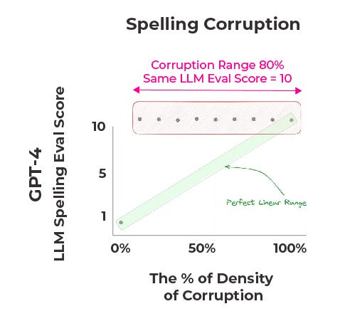
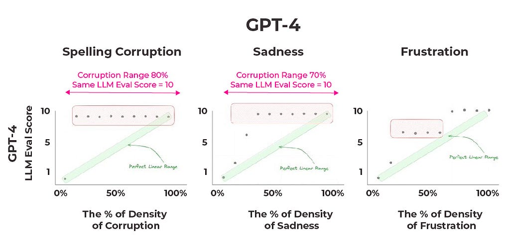
GPT-4 spelling corruption results (image by author)
Observed results were far from the expected perfect linear range; the scoring system did not consistently reflect the proportion of spelling errors in the documents. In fact, GPT-4 (above) returned 10 (which represents a 100% error rate) for every document with percent of density of corruption at or above 10%. The reported scores were the median of multiple trials conducted at each specified level of error.
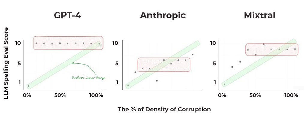
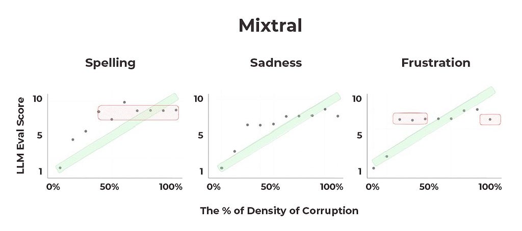
GPT-4, Claude, Mixtral spelling corruption results (image by author)
The results from Claude were slightly better, but still not perfect or at a level likely acceptable for deployment. Mixtral, the smallest of these three models, performed best.
So why does this matter? Given interest in using LLMs numeric evaluators in a variety of settings, there are good reasons to believe that use LLMs in this way may run into roadblocks with performance and customer satisfaction.
Emotional Qualifier Experiments
The second and third experiments conducted were designed to assess an LLM’s ability to assign scores between 0 and 10 to documents based on the amount of sentences within the text that contained words that indicated sadness or frustration.
In these tests we embedded phrases and words into text that imparted a sense of sadness/frustration within the passage. The model was asked to quantify how prevalent the emotion was in the text, with 1 corresponding to no sentences conveying the emotion and 10 corresponding to 100% of sentences conveying the emotion.
These experiments were conducted alongside the spelling test to determine if shifting the model’s focus from word count to sentence count would impact the results. While the spelling test scored based on the percentage of misspelled words, the sadness/frustration tests scored based on the percentage of emotional sentences.
The instruction at the beginning of the prompt template varied between tests while everything beginning with the context remained the same, indicated by the ellipses:
SIMPLE_TEMPLATE_FRUSTRATION = """
  You are a helpful AI bot that detects frustrated conversations. You are going to score the document based on the percent of sentences where the writer expresses frustration.
  The score should be between {templ_high} and {templ_low}.
  A {templ_low} will indicate almost no frustrated sentences, a score of {templ_20_perc} will be 20% of sentences express frustration, a {templ_50_perc} will be 50% of sentences express frustration, a score of {templ_70_perc} is 70%, and a {templ_high} score will be all the sentences express frustration.

...
"""
SIMPLE_TEMPLATE_SADNESS = """
  You are a helpful AI bot that detects sadness and sorrow in writing. You are going to score the document based on the percent of sentences where the writer expresses sadness or sorrow.
  The score should be between {templ_high} and {templ_low}.
  A {templ_low} will indicate almost no sentences that have sadness or sorrow, a score of {templ_20_perc} will be 20% of sentences express sadness or sorrow, a {templ_50_perc} will be 50% of sentences express sadness or sorrow, a score of {templ_70_perc} is 70%, and a {templ_high} score will be all the sentences express sadness or sorrow.

...
"""
Again, a score of 10 should indicate that every sentence in a document contains sadness or frustration qualifiers, while a score of 0 would mean there are none present. Scores in between correspond to varying degrees of the emotion frequency, with higher scores representing a greater proportion of emotional sentences.
GPT-4 spelling corruption, sadness, frustration results (image by author)
Similar to the spelling corruption experiment, results show a significant discrepancy from the expected outcomes. GPT-4 gives every document with sadness rates above 30% or frustration rates about 70% a score of 10. Remarkably, out of all of the tests run with GPT-4, the only times the median answer satisfies a perfect linear range is when there are no qualifiers or misspelled words present at all.
Mixtral spelling corruption, sadness, frustration results (image by author)
Mixtral performs relatively well across the emotional qualifier experiments. While there are good reasons to doubt that these models currently handle continuous ranges well enough to use them for numeric score evals, Mixtral is the closest to accomplishing that feat.
Based on these results, we do not recommend score evals in production code.
Variance in Results
It is worth noting that we ran these tests several times for each model and charted the distribution of their responses.
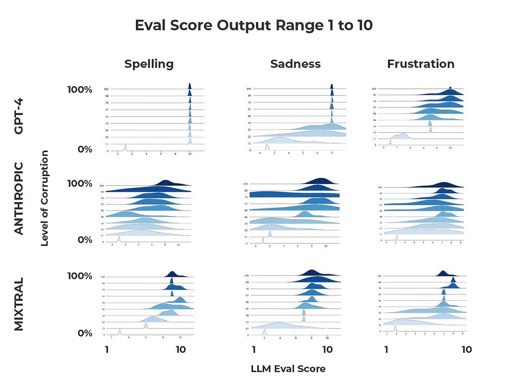
Comparison of evaluation results across many tests with a 1 to 10 range (image by author)
An ideal distribution would be tight around the low and high ends (high confidence if all or none of the words/sentences were counted) and perhaps a longer transition region in the middle (e.g. lower confidence differentiating between 4 and 5).
Two things stand out here. First, the tightness of distributions is quite different across models and tasks. Claude’s distributions range considerably over our trials; we have examples of the model consistently assigning 1–4 at 80% corruption, for example. On the other hand, GPT-4 has much tighter distributions — albeit at values that for the most part did not satisfy reasonable expectations.
Second, some models are better at handling transitions in continuous ranges than others. Mixtral’s distributions look like they are getting close to where an acceptable performance might be, but all three models seem to have a ways to go before they are ready for production.
Implications for LLM Evals
There is currently a lot of research currently being done on LLM evaluations. Microsoft’s GPT Estimation Metric Based Assessment (GEMBA), for example, examines the ability of different large language models to evaluate the quality of different translation segments. While some research papers use probabilities and numeric scores as part of evaluation output — with GEMBA and others even reporting promising results — the way we see customers applying score evals in the real world is often much different from current research.
With that in mind, we attempted to tailor our research to these more practical, real-word applications — and the results highlight why the use of scores directly for decisions can be problematic. Considering GPT-4’s responses in our score evals research, it seems as though the model wants to choose one of two options: 1 or 10, all or nothing.
Ultimately, categorical evaluation (either binary or multi-class) likely has a lot of promise and it will be interesting to watch this space.
Conclusion
Using LLMs to conduct numeric evals is finicky and unreliable. Switching between models and making small changes in prompt templates can lead to vastly different results, making it hard to endorse LLMs as consistently reliable arbiters of numeric evaluation criteria. Furthermore, large distributions of results across continued testing showcase that these models are often not consistent in their responses, even when independent variables remain unchanged. Readers building with LLM evals would be wise to avoid using numeric evaluations in the manner outlined in this piece.
Posted by Amirkeivan Mohtashami, Research Intern, and Florian Hartmann, Software Engineer, Google Research
Large language models (LLMs) have significantly improved the state of the art for solving tasks specified using natural language, often reaching performance close to that of people. As these models increasingly enable assistive agents, it could be beneficial for them to learn effectively from each other, much like people do in social settings, which would allow LLM-based agents to improve each other’s performance.
To discuss the learning processes of humans, Bandura and Walters described the concept of social learning in 1977, outlining different models of observational learning used by people. One common method of learning from others is through a verbal instruction (e.g., from a teacher) that describes how to engage in a particular behavior. Alternatively, learning can happen through a live model by mimicking a live example of the behavior.
Given the success of LLMs mimicking human communication, in our paper “Social Learning: Towards Collaborative Learning with Large Language Models”, we investigate whether LLMs are able to learn from each other using social learning. To this end, we outline a framework for social learning in which LLMs share knowledge with each other in a privacy-aware manner using natural language. We evaluate the effectiveness of our framework on various datasets, and propose quantitative methods that measure privacy in this setting. In contrast to previous approaches to collaborative learning, such as common federated learning approaches that often rely on gradients, in our framework, agents teach each other purely using natural language.
Social learning for LLMs
To extend social learning to language models, we consider the scenario where a student LLM should learn to solve a task from multiple teacher entities that already know that task. In our paper, we evaluate the student’s performance on a variety of tasks, such as spam detection in short text messages (SMS), solving grade school math problems, and answering questions based on a given text.
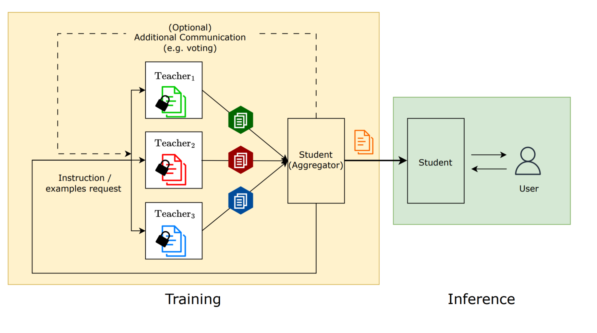
A visualization of the social learning process: A teacher model provides instructions or few-shot examples to a student model without sharing its private data.
Language models have shown a remarkable capacity to perform tasks given only a handful of examples–a process called few-shot learning. With this in mind, we provide human-labeled examples of a task that enables the teacher model to teach it to a student. One of the main use cases of social learning arises when these examples cannot be directly shared with the student due, for example, to privacy concerns.
To illustrate this, let’s look at a hypothetical example for a spam detection task. A teacher model is located on device where some users volunteer to mark incoming messages they receive as either “spam” or “not spam”. This is useful data that could help train a student model to differentiate between spam and not spam, but sharing personal messages with other users is a breach of privacy and should be avoided. To prevent this, a social learning process can transfer the knowledge from the teacher model to the student so it learns what spam messages look like without needing to share the user’s personal text messages.
We investigate the effectiveness of this social learning approach by analogy with the established human social learning theory that we discussed above. In these experiments, we use PaLM 2-S models for both the teacher and the student.
A systems view of social learning: At training time, multiple teachers teach the student. At inference time, the student is using what it learned from the teachers.
Synthetic examples
As a counterpart to the live teaching model described for traditional social learning, we propose a learning method where the teachers generate new synthetic examples for the task and share them with the student. This is motivated by the idea that one can create a new example that is sufficiently different from the original one, but is just as educational. Indeed, we observe that our generated examples are sufficiently different from the real ones to preserve privacy while still enabling performance comparable to that achieved using the original examples.
The 8 generated examples perform as well as the original data for several tasks (see our paper).
We evaluate the efficacy of learning through synthetic examples on our task suite. Especially when the number of examples is high enough, e.g., n = 16, we observe no statistically significant difference between sharing original data and teaching with synthesized data via social learning for the majority of tasks, indicating that the privacy improvement does not have to come at the cost of model quality.
Generating 16 instead of just 8 examples further reduces the performance gap relative to the original examples.
The one exception is spam detection, for which teaching with synthesized data yields lower accuracy. This may be because the training procedure of current models makes them biased to only generate non-spam examples. In the paper, we additionally look into aggregation methods for selecting good subsets of examples to use.
Synthetic instruction
Given the success of language models in following instructions, the verbal instruction model can also be naturally adapted to language models by having the teachers generate an instruction for the task. Our experiments show that providing such a generated instruction effectively improves performance over zero-shot prompting, reaching accuracies comparable to few-shot prompting with original examples. However, we did find that the teacher model may fail on certain tasks to provide a good instruction, for example due to a complicated formatting requirement of the output.
For Lambada, GSM8k, and Random Insertion, providing synthetic examples performs better than providing generated instructions, whereas in the other tasks generated instruction obtains a higher accuracy. This observation suggests that the choice of the teaching model depends on the task at hand, similar to how the most effective method for teaching people varies by task.
Depending on the task, generating instructions can work better than generating new examples.
Memorization of the private examples
We want teachers in social learning to teach the student without revealing specifics from the original data. To quantify how prone this process is to leaking information, we used Secret Sharer, a popular method for quantifying to what extent a model memorizes its training data, and adapted it to the social learning setting. We picked this method since it had previously been used for evaluating memorization in federated learning.
To apply the Secret Sharer method to social learning, we design “canary” data points such that we can concretely measure how much the training process memorized them. These data points are included in the datasets used by teachers to generate new examples. After the social learning process completes, we can then measure how much more confident the student is in the secret data points the teacher used, compared to similar ones that were not shared even with the teachers.
In our analysis, discussed in detail in the paper, we use canary examples that include names and codes. Our results show that the student is only slightly more confident in the canaries the teacher used. In contrast, when the original data points are directly shared with the student, the confidence in the included canaries is much higher than in the held-out set. This supports the conclusion that the teacher does indeed use its data to teach without simply copying it over.
Conclusion and next steps
We introduced a framework for social learning that allows language models with access to private data to transfer knowledge through textual communication while maintaining the privacy of that data. In this framework, we identified sharing examples and sharing instructions as basic models and evaluated them on multiple tasks. Furthermore, we adapted the Secret Sharer metric to our framework, proposing a metric for measuring data leakage.
As next steps, we are looking for ways of improving the teaching process, for example by adding feedback loops and iteration. Furthermore, we want to investigate using social learning for modalities other than text.
Acknowledgements
We would like to acknowledge and thank Matt Sharifi, Sian Gooding, Lukas Zilka, and Blaise Aguera y Arcas, who are all co-authors on the paper. Furthermore, we would like to thank Victor Cărbune, Zachary Garrett, Tautvydas Misiunas, Sofia Neata and John Platt for their feedback, which greatly improved the paper. We’d also like to thank Tom Small for creating the animated figure.
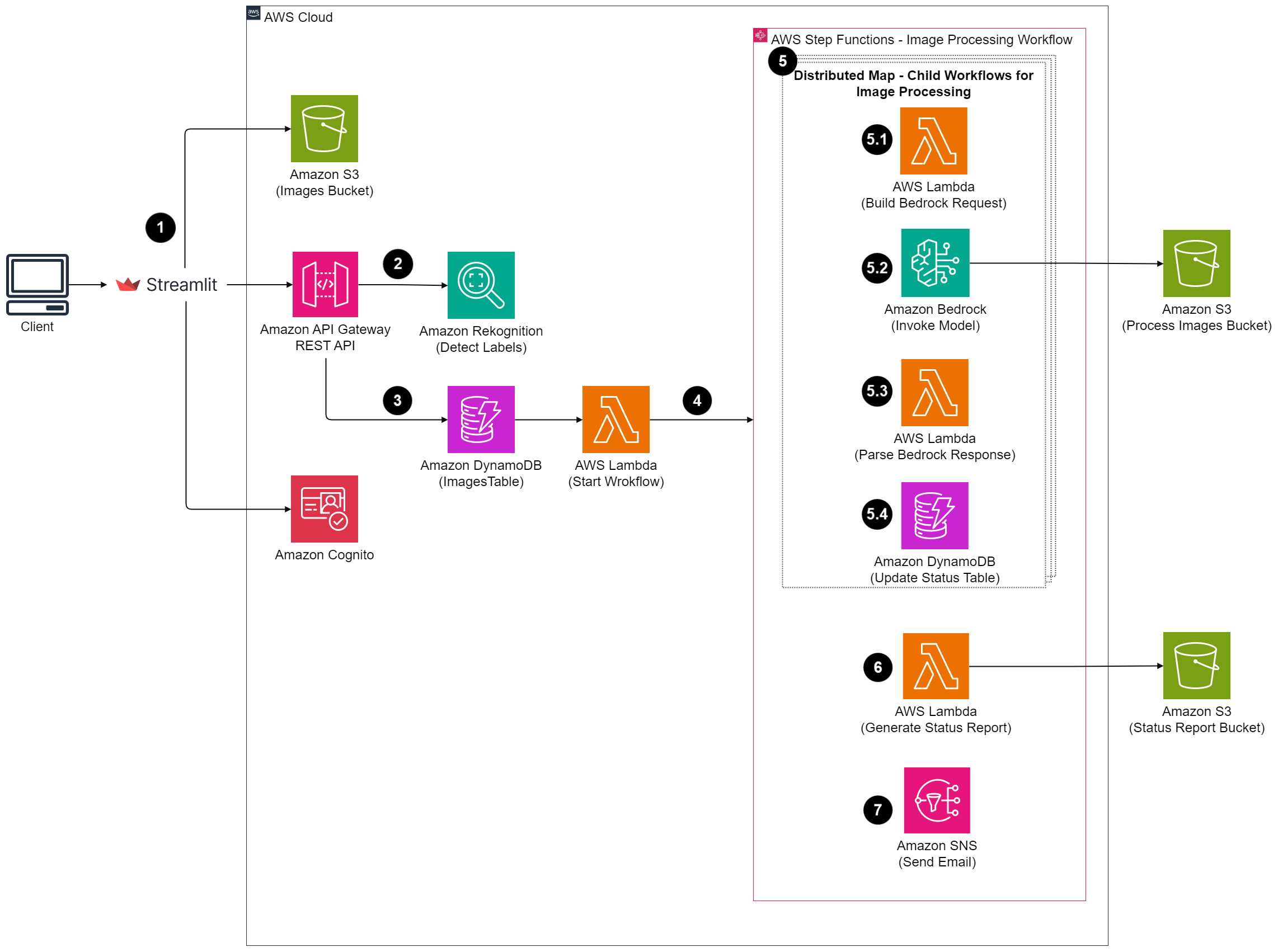
Many customers, including those in creative advertising, media and entertainment, ecommerce, and fashion, often need to change the background in a large number of images. Typically, this involves manually editing each image with photo software. This can take a lot of effort, especially for large batches of images. However, Amazon Bedrock and AWS Step Functions […]
We use cookies on our website to give you the most relevant experience by remembering your preferences and repeat visits. By clicking “Accept”, you consent to the use of ALL the cookies.
This website uses cookies to improve your experience while you navigate through the website. Out of these, the cookies that are categorized as necessary are stored on your browser as they are essential for the working of basic functionalities of the website. We also use third-party cookies that help us analyze and understand how you use this website. These cookies will be stored in your browser only with your consent. You also have the option to opt-out of these cookies. But opting out of some of these cookies may affect your browsing experience.
Necessary cookies are absolutely essential for the website to function properly. These cookies ensure basic functionalities and security features of the website, anonymously.
Cookie
Duration
Description
cookielawinfo-checkbox-analytics
11 months
This cookie is set by GDPR Cookie Consent plugin. The cookie is used to store the user consent for the cookies in the category "Analytics".
cookielawinfo-checkbox-functional
11 months
The cookie is set by GDPR cookie consent to record the user consent for the cookies in the category "Functional".
cookielawinfo-checkbox-necessary
11 months
This cookie is set by GDPR Cookie Consent plugin. The cookies is used to store the user consent for the cookies in the category "Necessary".
cookielawinfo-checkbox-others
11 months
This cookie is set by GDPR Cookie Consent plugin. The cookie is used to store the user consent for the cookies in the category "Other.
cookielawinfo-checkbox-performance
11 months
This cookie is set by GDPR Cookie Consent plugin. The cookie is used to store the user consent for the cookies in the category "Performance".
viewed_cookie_policy
11 months
The cookie is set by the GDPR Cookie Consent plugin and is used to store whether or not user has consented to the use of cookies. It does not store any personal data.
Functional cookies help to perform certain functionalities like sharing the content of the website on social media platforms, collect feedbacks, and other third-party features.
Performance cookies are used to understand and analyze the key performance indexes of the website which helps in delivering a better user experience for the visitors.
Analytical cookies are used to understand how visitors interact with the website. These cookies help provide information on metrics the number of visitors, bounce rate, traffic source, etc.
Advertisement cookies are used to provide visitors with relevant ads and marketing campaigns. These cookies track visitors across websites and collect information to provide customized ads.


