A step-by-step guide for setting up an RStudio server inside a container with your local RStudio settings
This is a step-by-step guide for setting up an RStudio server inside a container with your local RStudio settings. We will use the Rocker RStudio image and show how to customize it with the docker run command and its arguments.
By the end of this tutorial, you will be able to:
Launch an RStudio server inside a container
Mount local folders
Clone local RStudio settings (color theme, code snippets, etc.)
Load local Renviron setting
A whale carries an R container (created by the author with Midjourney)
Introduction
RStudio is the primary IDE for the R programming language. Unlike other general-purpose IDEs such as VScode, RStudio was built and designed specifically for R users and their needs. This is one of the reasons for the popularity of RStudio among R users. By default, RStudio does not have native support for Docker. The main method for setting and running RStudio inside a container is using the RStudio server version. This required installing and setting the server inside a container, which might be an entry barrier for some users. Luckily, the Rocker project — the main source for R images provides built-in and ready-to-use images with an RStudio server.
Throughout this tutorial, we will use the Rocker RStudio image, which is available on Docker Hub.
Prerequisites
To follow along with this tutorial and run the code below, you will need:
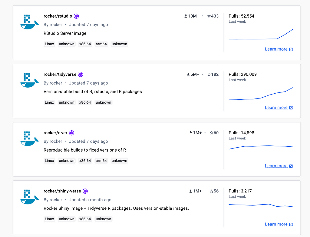
The Rocker Project is the main hub for built-in R images. It provides various images with different R environment settings, such as base-r, tidyverse, ML-verse, shiny, geospatial, and, of course, the RStudio server image. The full list of available R images is on the Rocker’s Docker Hub page.
Rocker’s top images by number of downloads (screenshot from Docker Hub by the author)
We will use the rocker/rstudio image, which, as its name implies, has an RStudio server installed and ready to use. Using thedocker run command, we can launch this container in an interactive mode and access the RStudio server via the browser.
Let’s get started by pulling the image with the docker pull command:
You can use the docker images command to verify that the image was downloaded successfully:
>docker images                                                                                                                                                    ok  36s
REPOSITORY              TAG          IMAGE ID       CREATED       SIZE
rocker/rstudio          latest       7039fb162243   2 days ago    1.94GB
Let’s now go ahead and use the suggested command from the Rocker Project to launch RStudio inside the container with the docker run command:
>docker run --rm -ti -e PASSWORD=yourpassword -p 8787:8787 rocker/rstudio
Before we open the RStudio server on the browser, let’s review the run arguments we used above:
rm — Automatically remove the container when it exits (from the terminal control + c)
ti — Run the container in an interactive mode
e — Set environment variable, in this case, to define the server login password as yourpassword
p — Define the port mapping. In this case, we will map the container’s 8787 port with port 8787 on the local machine
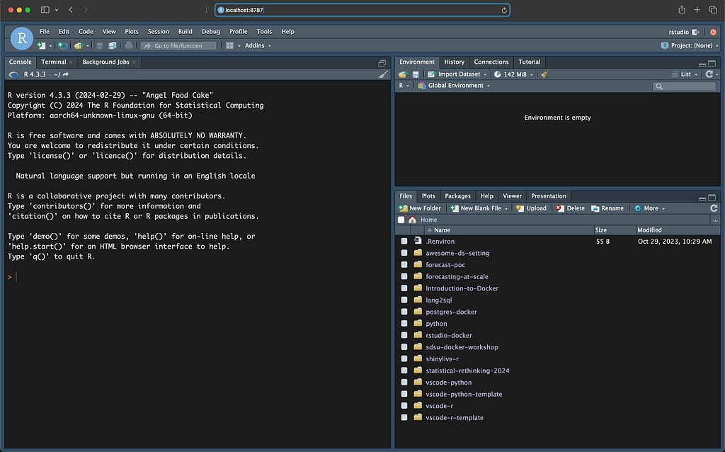
After running the command, you can access the RStudio server on local host 8787 (e.g., http://localhost:8787). This will prompt the login page, where you should use:
Username: rstudio
Password: yourpassword (as set in the run commend)
You should expect the following output:
The initial view of the RStudio server (screenshot by the author)
Note: You can stop the running container on terminal by clicking control+c.
Oh No! It Is Ephemeral!
By default, the Docker container runs in ephemeral mode. Any code created and saved on the container or input you generated will be lost when terminating the container run time. This is neither practical nor useful if you wish to use Docker as your development environment. To address this issue, we will use the volume (or v)argument, which enables the mount of local folders with the container files system.
The below code demonstrates the use of the volume argument to mount the folder we execute the run command from (e.g., .) with the RStudio server home folder:
The volume argument maps the local folder (e.g., source) with the container (e.g., target) using the following format source:target.
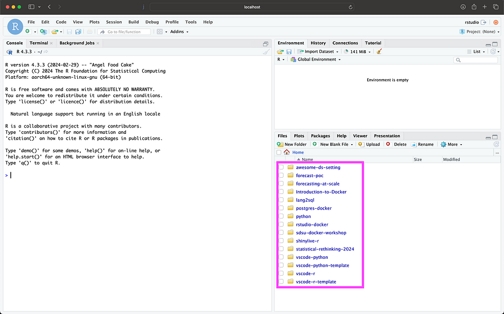
Let’s now go back to the browser and reopen the RStudio server using the local host address — http://localhost:8787. You should expect to see in the RStudio files section the folders and/or files that are available on the local folder you mount to the container. In my case, I will mount my tutorials folder, which has the following folders:
As you can see in the screenshot below, the local folders are now available and accessible from the RStudio server (marked with a purple rectangle):
RStudio server with a local volume (screenshot by the author)
Note: You can use the volume argument to mount multiple volumes. For example, one for your project and second for a folder with your data folders
This enables us to read from and write to the local folder from the container during run time.
Clone Your Local RStudio Settings
In the previous section, we saw how to mount a local folder to the container with the volume argument. This enables us to save our code locally while working inside the container. In this section, we will see how we can leverage the volume argument to mount our local RStudio setting with the ones on the container. The idea here is to launch the container and run the RStudio server with our local settings without needing to update the settings any time we relaunch the container. This includes loading local settings such as color theme settings, code snippets, environment variables, etc.
Before we can update the docker run with the local RStudio configuration folder, we need to identify the folder path of the config folder of both the local and the one on the container. For example, the path on my machine is ~/.config/rstudio and it contains the following folders and files:
Likewise, we want to mount the .Renviron file with the local environment variables. The .Renviron file is under the root folder on the local machine, and we follow the same approach to map the local file with the ones on the container:
$HOME/.Renviron:/home/rstudio/.Renviron
Let’s now add it all together and relaunch the container:
After mounting the local RStudio config folder with the one on the container, the server settings are now mapped with the local RStudio settings on my machine:
RStudio server with the local settings (screenshot by the author)
Summary
This tutorial focuses on customizing the Rocker’s RStudio image with the docker run command. We used the volume argument to mount the local folder to the container working directory. This enables us to work inside a containerized environment and save our work locally. In addition, we used the volume argument to clone the local RStudio settings to the container. This makes the transition from the local environment to the containerized smoother. The command can become long and convoluted as we add and use more arguments. Once you have finalized your run settings, the next step is to transition it into a YAML file using the Docker Compose. Beyond the simplification of the launch process of the container, Docker Compose enables you to manage more complex scenarios, such as launching multiple containers.
Simple Python code for accessing Sun RGB-D and similar datasets
3D understanding from 2D images is the first step into a larger world.
As many of the primitive tasks in computer vision approach a solved state — decent, quasi-general solutions now being available for image segmentation and text-conditioned generation, with general answers to visual question answering, depth estimation, and general object detection well on the way — I and many of my colleagues have been looking to use CV in larger tasks. When a human looks at a scene, we see more than flat outlines. We comprehend more than a series of labels. We can perceive and imagine within 3D spaces. We see a scene, and we can understand it in a very complete way. This capability should be within reach for CV systems of the day… If only we had the right data.
Sun RGB-D is an interesting image dataset from 2015 that satiates many of the data hungers of total scene understanding. This dataset is a collection of primarily indoor scenes, collected with a digital camera and four different 3D scanners. The linked publication goes into greater detail on how the dataset was collected and what it contains. Most importantly though, this dataset contains a wealth of data that includes both 2D and 3D annotations.
With this dataset, CV and ML algorithms can learn much deeper (excuse the pun) features from 2D images. More than that though, using data like this could open opportunities in applying 3D reasoning to 2D images. But that is a story for another time. This article will simply provide the basic python code to access this Sun RGB-D data, so that readers can use this wonderful resource in their own projects.
Dataset Layout
After downloading the dataset from here, you will end up with a directory structure like this.
These separate the data by the type of scanner used to collect them. Specifically, the Intel RealSense 3D Camera for tablets, the Asus Xtion LIVE PRO for laptops, and the Microsoft Kinect versions 1 and 2 for desktop.
Moving into “kv2”, we see two directories: align_kv2 and kinect2data. This is one problem with the Sun RGB-D dataset… its directory structure is not consistent for each sensor type. In “realsense”, there are four directories containing data: lg, sa, sh, and shr. In “xtion” there is a more complex directory structure still. And worse, I have been unable to find a clear description of how these sub-directories are different anywhere in the dataset’s paper, supplementary materials, or website. If anyone knows the answer to this, please let me know!
For the time being though, lets skip down into the consistent part of the dataset: the data records. For align_kv2, we have this:
For all of the data records across all of the sensor types, this part is largely consistent. Some important files to look at are described below:
annotation2Dfinal contains the most recent 2D annotations including polygonal object segmentations and object labels. These are stored in a single JSON file which has the x and y 2D coordinates for each point in each segmentation, as well as a list for object labels.
annotation3Dfinal is the same for 3D annotations. These are in the form of bounding shapes — polyhedra that are axis-aligned on the y (up-down) dimension. These can also be found in the singular JSON file of the directory.
depth contains the raw depth images collected by the sensor. depth_bfx contains a cleaned-up copy that addresses some of the limitations from the sensor.
The original image can be found in the image directory. A full resolution, uncropped version can also be found in fullres.
Sensor extrinsics and intrinsics are saved in text files as numpy-like arrays. intrinsics.txt contains the intrinsics, but extrinsics is stored in the singular text file within the extrinsics folder.
Finally, the type of scene (office, kitchen, bedroom, etc) can be found as a string in scene.txt.
Setup
First things first, we will need to read in files from a few formats. JSON and txt primarily. From those text files, we need to pull out a numpy array for both the extrinsics and intrinsics of the sensor. There are also allot of files here that don’t seem to follow a strict naming convention but will be the only one of its type in the same directory, so get_first_file_path will be useful here.
I’d also like this code to output a simple 3D model of the rooms we find in the dataset. This can give us some easy data visualization, and lets us distill down the basic spatial features of a scene. To achieve this, we’ll utilize the OBJ file format, a standard for representing 3D geometry. An OBJ file primarily consists of lists of vertices (points in 3D space), along with information on how these vertices are connected to form faces (the surfaces of the 3D object). The layout of an OBJ file is straightforward, beginning with vertices, each denoted by a line starting with ‘v’ followed by the x, y, and z coordinates of the vertex. Faces are then defined by lines starting with ‘f’, listing the indices of the vertices that form each face’s corners, thus constructing the 3D surface.
In our context, the bounding shapes that define the spatial features of a scene are polyhedra, 3D shapes with flat faces and straight edges. Given that the y dimension is axis-aligned — meaning it consistently represents the up-down direction across all points — we can simplify the representation of our polyhedron using only the x and z coordinates for defining the vertices, along with a global minimum (min_y) and maximum (max_y) y-value that applies to all points. This approach assumes that vertices come in pairs where the x and z coordinates remain the same while the y coordinate alternates between min_y and max_y, effectively creating vertical line segments.
The write_obj function encapsulates this logic to construct our 3D model. It starts by iterating over each bounding shape in our dataset, adding vertices to the OBJ file with their x, y, and z coordinates. For each pair of points (with even indices representing min_y and odd indices representing max_y where x and z are unchanged), the function writes face definitions to connect these points, forming vertical faces around each segment (e.g., around vertices 0, 1, 2, 3, then 2, 3, 4, 5, and so on). If the bounding shape has more than two pairs of vertices, a closing face is added to connect the last pair of vertices back to the first pair, ensuring the polyhedron is properly enclosed. Finally, the function adds faces for the top and bottom of the polyhedron by connecting all min_y vertices and all max_y vertices, respectively, completing the 3D representation of the spatial feature.
Finally, lets make the basic structure of our dataset, with a class that represents a dataset (a directory with subdirectories each containing a data record) and the data records themselves. This first object has a very simple function: it will create a new record object for every sub-directory within ds_dir.
Accessing 2D Segmentations
Accessing 2D segmentation annotations is easy enough. We must make sure to load the json file in annotation2Dfinal. Once that is loaded as a python dict, we can extract the segmentation polygons for each object in the scene. These polygons are defined by their x and y coordinates, representing the vertices of the polygon in the 2D image space.
We also extract the object label by storing the object ID that each bounding shape contains, then cross-referencing with the ‘objects’ list. Both the labels and segmentations are returned by get_segments_2d.
Note that the transpose operation is applied to the coordinates array to shift the data from a shape that groups all x coordinates together and all y coordinates together into a shape that groups each pair of x and y coordinates together as individual points.
Accessing 3D Bounding Shapes
Accessing the 3D bounding shapes is a bit harder. As mentioned before, they are stored as y-axis aligned polyhedra (x is left-right, z is forward-back, y is up-down). In the JSON, this is stored as a polygon with an min_y and max_y. This can be extracted to a polyhedron by taking each 2D point of the polygon, and adding two new 3D points with min_y and max_y.
The JSON also provides a useful field which states whether the bounding shape is rectangular. I have preserved this in our code, along with functions to get the type of each object (couch, chair, desk, etc), and the total number of objects visible in the scene.
Accessing the Room Layout
Finally, the room layout has its own polyhedron that encapsulates all others. This can be used by algorithms to understand the broader topology of the room including the walls, ceiling, and floor. It is accessed in much the same way as the other bounding shapes.
Full Code
Below is the full code with a short testing section. Besides visualizing the 2D annotations from one of the data records, we also save 3d .obj files for each identified object in the scene. You can use a program like meshlab to visualize the output. The sensor intrinsics and extrinsics have also been extracted here. Intrinsics refer to the internal camera parameters that affect the imaging process (like focal length, optical center, and lens distortion), while extrinsics describe the camera’s position and orientation in a world coordinate system. They are important for accurately mapping and interpreting 3D scenes from 2D images.
This repo may or may not be updated in the future. I would love to add functionality for accessing this as a PyTorch dataset with minibatches and such. If anyone has some easy updates, feel free to make a PR.
Left: the simple 3D representation of the scene shown in meshlab. Note the transparent room bounding shape and the many objects represented as boxes. Right: the original image.
Conclusion
I hope this guide has been helpful in showing you how to use the Sun RGB-D Dataset. More importantly, I hope it’s given you a peek into the broader skill of writing quick and easy code to access datasets. Having a tool ready to go is great, but understanding how that tool works and getting familiar with the dataset’s structure will serve you better in most cases.
Extra Notes
This article has introduced some easy-to-modify python code for extracting data from the Sun RGB-D dataset. Note that an official MATLAB toolbox for this dataset already exists. But I don’t use MATLAB so I didn’t look at it. If you are a MATLABer (MATLABster? MATLABradour? eh…) then that might be more comprehensive.
I also found this for python. It’s a good example of extracting only the 2D features. I borrowed some lines from it, so go throw it a star if you feel up to it.
References
This article utilizes the Sun RGB-D dataset [1] licensed under CC-BY-SA. This dataset also draws data from previous work [2, 3, 4]. Thank you to them for their outstanding contributions.
[1] S. Song, S. Lichtenberg, and J. Xiao, “SUN RGB-D: A RGB-D Scene Understanding Benchmark Suite,” Proceedings of the 28th IEEE Conference on Computer Vision and Pattern Recognition (CVPR2015), Oral Presentation.
[2] N. Silberman, D. Hoiem, P. Kohli, R. Fergus, “Indoor segmentation and support inference from RGBD images,” ECCV, 2012.
[3] A. Janoch, S. Karayev, Y. Jia, J. T. Barron, M. Fritz, K. Saenko, T. Darrell, “A category-level 3-D object dataset: Putting the Kinect to work,” ICCV Workshop on Consumer Depth Cameras for Computer Vision, 2011.
[4] J. Xiao, A. Owens, A. Torralba, “SUN3D: A database of big spaces reconstructed using SfM and object labels,” ICCV, 2013.
Posted by Dave Steiner, Clinical Research Scientist, Google Health, and Rory Pilgrim, Product Manager Google Research
There’s a worldwide shortage of access to medical imaging expert interpretation across specialties including radiology, dermatology and pathology. Machine learning (ML) technology can help ease this burden by powering tools that enable doctors to interpret these images more accurately and efficiently. However, the development and implementation of such ML tools are often limited by the availability of high-quality data, ML expertise, and computational resources.
One way to catalyze the use of ML for medical imaging is via domain-specific models that utilize deep learning (DL) to capture the information in medical images as compressed numerical vectors (called embeddings). These embeddings represent a type of pre-learned understanding of the important features in an image. Identifying patterns in the embeddings reduces the amount of data, expertise, and compute needed to train performant models as compared to working with high-dimensional data, such as images, directly. Indeed, these embeddings can be used to perform a variety of downstream tasks within the specialized domain (see animated graphic below). This framework of leveraging pre-learned understanding to solve related tasks is similar to that of a seasoned guitar player quickly learning a new song by ear. Because the guitar player has already built up a foundation of skill and understanding, they can quickly pick up the patterns and groove of a new song.
Path Foundation is used to convert a small dataset of (image, label) pairs into (embedding, label) pairs. These pairs can then be used to train a task-specific classifier using a linear probe, (i.e., a lightweight linear classifier) as represented in this graphic, or other types of models using the embeddings as input.
Once the linear probe is trained, it can be used to make predictions on embeddings from new images. These predictions can be compared to ground truth information in order to evaluate the linear probe’s performance.
In order to make this type of embedding model available and drive further development of ML tools in medical imaging, we are excited to release two domain-specific tools for research use: Derm Foundation and Path Foundation. This follows on the strong response we’ve already received from researchers using the CXR Foundation embedding tool for chest radiographs and represents a portion of our expanding research offerings across multiple medical-specialized modalities. These embedding tools take an image as input and produce a numerical vector (the embedding) that is specialized to the domains of dermatology and digital pathology images, respectively. By running a dataset of chest X-ray, dermatology, or pathology images through the respective embedding tool, researchers can obtain embeddings for their own images, and use these embeddings to quickly develop new models for their applications.
Path Foundation
In “Domain-specific optimization and diverse evaluation of self-supervised models for histopathology”, we showed that self-supervised learning (SSL) models for pathology images outperform traditional pre-training approaches and enable efficient training of classifiers for downstream tasks. This effort focused on hematoxylin and eosin (H&E) stained slides, the principal tissue stain in diagnostic pathology that enables pathologists to visualize cellular features under a microscope. The performance of linear classifiers trained using the output of the SSL models matched that of prior DL models trained on orders of magnitude more labeled data.
Due to substantial differences between digital pathology images and “natural image” photos, this work involved several pathology-specific optimizations during model training. One key element is that whole-slide images (WSIs) in pathology can be 100,000 pixels across (thousands of times larger than typical smartphone photos) and are analyzed by experts at multiple magnifications (zoom levels). As such, the WSIs are typically broken down into smaller tiles or patches for computer vision and DL applications. The resulting images are information dense with cells or tissue structures distributed throughout the frame instead of having distinct semantic objects or foreground vs. background variations, thus creating unique challenges for robust SSL and feature extraction. Additionally, physical (e.g., cutting) and chemical (e.g., fixing and staining) processes used to prepare the samples can influence image appearance dramatically.
Taking these important aspects into consideration, pathology-specific SSL optimizations included helping the model learn stain-agnostic features, generalizing the model to patches from multiple magnifications, augmenting the data to mimic scanning and image post processing, and custom data balancing to improve input heterogeneity for SSL training. These approaches were extensively evaluated using a broad set of benchmark tasks involving 17 different tissue types over 12 different tasks.
Utilizing the vision transformer (ViT-S/16) architecture, Path Foundation was selected as the best performing model from the optimization and evaluation process described above (and illustrated in the figure below). This model thus provides an important balance between performance and model size to enable valuable and scalable use in generating embeddings over the many individual image patches of large pathology WSIs.
SSL training with pathology-specific optimizations for Path Foundation.
Path Foundation embeddings significantly outperform traditional ImageNet embeddings as evaluated by linear probing across multiple evaluation tasks in histopathology.
Derm Foundation
Derm Foundation is an embedding tool derived from our research in applying DL to interpret images of dermatology conditions and includes our recent work that adds improvements to generalize better to new datasets. Due to its dermatology-specific pre-training it has a latent understanding of features present in images of skin conditions and can be used to quickly develop models to classify skin conditions. The model underlying the API is a BiT ResNet-101×3 trained in two stages. The first pre-training stage uses contrastive learning, similar to ConVIRT, to train on a large number of image-text pairs from the internet. In the second stage, the image component of this pre-trained model is then fine-tuned for condition classification using clinical datasets, such as those from teledermatology services.
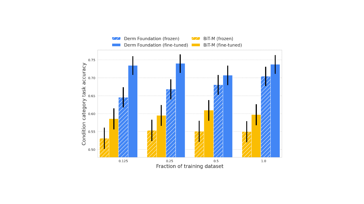
Unlike histopathology images, dermatology images more closely resemble the real-world images used to train many of today’s computer vision models. However, for specialized dermatology tasks, creating a high-quality model may still require a large dataset. With Derm Foundation, researchers can use their own smaller dataset to retrieve domain-specific embeddings, and use those to build smaller models (e.g., linear classifiers or other small non-linear models) that enable them to validate their research or product ideas. To evaluate this approach, we trained models on a downstream task using teledermatology data. Model training involved varying dataset sizes (12.5%, 25%, 50%, 100%) to compare embedding-based linear classifiers against fine-tuning.
The modeling variants considered were:
A linear classifier on frozen embeddings from BiT-M (a standard pre-trained image model)
Fine-tuned version of BiT-M with an extra dense layer for the downstream task
A linear classifier on frozen embeddings from the Derm Foundation API
Fine-tuned version of the model underlying the Derm Foundation API with an extra layer for the downstream task
We found that models built on top of the Derm Foundation embeddings for dermatology-related tasks achieved significantly higher quality than those built solely on embeddings or fine tuned from BiT-M. This advantage was found to be most pronounced for smaller training dataset sizes.
These results demonstrate that the Derm Foundation tooI can serve as a useful starting point to accelerate skin-related modeling tasks. We aim to enable other researchers to build on the underlying features and representations of dermatology that the model has learned.
However, there are limitations with this analysis. We’re still exploring how well these embeddings generalize across task types, patient populations, and image settings. Downstream models built using Derm Foundation still require careful evaluation to understand their expected performance in the intended setting.
Access Path and Derm Foundation
We envision that the Derm Foundation and Path Foundation embedding tools will enable a range of use cases, including efficient development of models for diagnostic tasks, quality assurance and pre-analytical workflow improvements, image indexing and curation, and biomarker discovery and validation. We are releasing both tools to the research community so they can explore the utility of the embeddings for their own dermatology and pathology data.
To get access, please sign up to each tool’s terms of service using the following Google Forms.
After gaining access to each tool, you can use the API to retrieve embeddings from dermatology images or digital pathology images stored in Google Cloud. Approved users who are just curious to see the model and embeddings in action can use the provided example Colab notebooks to train models using public data for classifying six common skin conditions or identifying tumors in histopathology patches. We look forward to seeing the range of use-cases these tools can unlock.
Acknowledgements
We would like to thank the many collaborators who helped make this work possible including Yun Liu, Can Kirmizi, Fereshteh Mahvar, Bram Sterling, Arman Tajback, Kenneth Philbrik, Arnav Agharwal, Aurora Cheung, Andrew Sellergren, Boris Babenko, Basil Mustafa, Jan Freyberg, Terry Spitz, Yuan Liu, Pinal Bavishi, Ayush Jain, Amit Talreja, Rajeev Rikhye, Abbi Ward, Jeremy Lai, Faruk Ahmed, Supriya Vijay,Tiam Jaroensri, Jessica Loo, Saurabh Vyawahare, Saloni Agarwal, Ellery Wulczyn, Jonathan Krause, Fayaz Jamil, Tom Small, Annisah Um’rani, Lauren Winer, Sami Lachgar, Yossi Matias, Greg Corrado, and Dale Webster.
A survey of recent developments in vision and multimodal models along with considerations for leaders as they position their organizations to capitalize on the coming wave of AI fueled change.
Photo created by DALL-E
I. Introduction
The past 18 months have ushered in tremendous change that is disrupting the very nature of work. Generative Artificial Intelligence (GenAI), Large Language Models (LLMs), and foundation models have become ubiquitous in vernacular. These models, containing billions of parameters and trained on massive amounts of data using self-supervised methods, are performing complex natural language tasks and exhibiting more generalized intelligence compared to earlier models [i][ii]; fueling unparallel productivity gains across diverse industries through numerous use cases such as personalized customer care and self-service [iii], knowledge management [iv] and content creation [v], research and development [vi], fraud detection [vii][viii], language translation [ix], and even forecasting of life expectancy [x].
Closely following in this wake are emerging developments in computer vision methods and approaches. At the forefront of this shift are advancements in vision transformer (ViT) architectures that are propelling computer vision capabilities into unprecedented levels of sophistication. Awareness of the rapid development and maturation of these capabilities is crucial to navigating the rapidly evolving AI landscape. Now, more than ever, defense leaders need to understand and harness these capabilities within Processing, Exploitation, and Dissemination (PED) and mission planning workflows to enable sensemaking at scale.
II. Rise of the Vision Transformer Architecture
Convolutional neural networks (CNNs) [xi] have traditionally held dominance within computer vision, demonstrating high performance on common tasks such as image classification, object detection, and segmentation. However, training such models requires significant amounts of labeled data for supervised learning, a highly labor-intensive task that is challenging to scale and slow to adapt to dynamic changes in the environment or requirements. Furthermore, the labeled datasets that do exist in the public domain may frequently be unsuitable to the unique use cases and/or imagery types that exist within the national security domain.
Recent years have seen the inception of the ViT architecture as a leading contender in the computer vision arena. The power of ViTs is in their ability to decompose images into fixed size patches and encode these fragments into a linear sequence of embeddings that capture semantic representations, similar to a sentence that describes the image. The ViT then sequentially understands each fragment, applying multi-head self-attention to recognize patterns and capture relationships globally across all fragments, to build a coherent understanding of the image [xii].
This results in several benefits over CNNs. First and foremost, ViTs are shown to demonstrate performance that matches or exceeds the state of the art compared to CNNs on many image classification datasets when trained on large quantities of data (e.g., 14 million — 300 million images). This level of performance is achieved while requiring 2–4 times less compute to train. In addition, ViTs can natively handle images of varying dimension due to their ability to process arbitrary sequence lengths (within memory constraints). Lastly, ViTs can capture long-range dependencies between inputs and provide enhanced scalability over CNNs. ViTs do have some limitations in comparison to CNNs. ViTs are unable to generalize well when trained on insufficient data due to lacking strong inductive biases, such as translation equivariance and locality. As a result, CNNs outperform ViTs on smaller datasets. However, when considering the scaling challenges present within DoD, ViTs show promise as an architecture to lead in this space.
2023 saw several computer vision advances leveraging ViT architectures. While in no way exhaustive, four models that highlight the rapid evolution of computer vision are Distillation of Knowledge with No Labels Version 2 (DINOv2), the Segment Anything Model (SAM), the Joint-Embedding Predictive Architecture (JEPA), and the Prithvi geospatial foundation model.
DINOv2 [xiii] leverages two concepts that advanced computer vision. The first concept is that of self-supervised learning of visual features directly from images, removing the need for large quantities of labels to support model training. Central to this approach is DINOv2’s data processing pipeline, which clusters images from a large uncurated dataset with images from a smaller curated dataset through a self-supervised retrieval system. This process results in the ability to create a large augmented curated dataset without a drop in quality, a key hurdle that must be crossed in scaling image foundation models. Additionally, DINOv2 employs a teacher-student distillation method to transfer knowledge from a large model to smaller models. At a high level, this approach works by freezing the weights of the large model with the goal of minimizing the differences between the embeddings coming from the smaller models with that of the larger model. This method is shown to achieve better performance than attempting to train smaller models directly on the data. Once trained, DINOv2 learned features demonstrate very good transferability across domains and the ability understand relations between similar parts of different objects. This results in an image foundation model whose outputs can be used by multiple downstream models for specific tasks.
SAM [xiv] is an image segmentation foundation model capable of promptable zero-shot segmentation of unfamiliar objects and images, without the need for additional training. This is accomplished through an architecture with three components: a ViT image encoder, a prompt encoder able to support both sparse (e.g., points, boxes, text) and dense (i.e., mask) prompts, and a fast mask decoder that efficiently maps the image embedding, prompt embeddings, and an output token to an autogenerated image mask. SAM is not without limitations as it requires large-scale supervised training, can miss fine structures, suffer from minor hallucinations, and may not produce boundaries as crisp as other methods. However, initial efforts present opportunity to address mission use cases that require the ability to segment objects in imagery.
Originally adapted to image tasks, JEPA [xv] is the first computer vision architecture designed to address critical shortcomings in existing ML systems needed to reach human levels of learning and understanding of the external world [xvi]. JEPA attempts to overcome limitations with current self-supervised learning methods (e.g., invariance-based methods, generative methods) through predicting missing image information in an abstract representation space. In practice, this is performed by predicting the representations (e.g., embeddings) of various target blocks (e.g., tail, legs, ears) in an image based on being provided a single context block (e.g., body and head of a dog). By predicting semantic representations of target blocks, without explicitly predicting the image pixels, JEPA is able to more closely replicate how humans predict missing parts of an image. More importantly, JEPA’s performance is comparable with invariance-based methods on semantic tasks, performs better on low-level vision tasks (e.g., object counting), and demonstrates high scalability and computational efficiency. This model architecture is continuing to be advanced with the introduction of latent variable energy-based models [xvii] to achieve multimodal predictions in high-dimensional problems with significant uncertainty (e.g., autonomous system navigation) and has recently been adapted to video [xviii].
Lastly, IBM, through a public/private partnership involving NASA and IBM Research, developed the first open-source geospatial foundation model for remote sensing data called Prithvi [xix]. Model development leveraged a First-of-a-Kind framework to build a representative dataset of raw multi-temporal and multi-spectral satellite images that avoided biases toward the most common geospatial features and removed noise from cloud cover or missing data from sensor malfunctions. This dataset was then used for self-supervised foundation model pretraining using an encoder-decoder architecture based on the masked autoencoder (MAE) [xx] approach. Prithvi was subsequently fined tuned using a small set of labeled images for specific downstream tasks, such as multi-temporal cloud imputation, flood mapping, fire-scar segmentation, and multi-temporal crop segmentation. Importantly, Prithvi is shown to generalize to different resolutions and geographic regions from the entire globe using a few labeled data during fine-tuning and is being used to convert NASA’s satellite observations into customized maps of natural disasters and other environmental changes.
III. Rapid Evolution: AI Trends in Flux
2023 also introduced the convergence of LLMs and ViTs (along with other modes) into Large Multimodal Models (LMMs), also referred to as vision language models (VLM) or multimodal large language models (MLLM). The strength of these models lies in their ability to combine the understanding of text with the interpretation of visual data [xxi]. However, this is not without challenges as training large multimodal models in an end-to-end manner would be immensely costly and risk catastrophic forgetting. In practice, training such models generally involves a learnable interface between a pre-trained visual encoder and an LLM [xxii].
Several influential models were released, to include Google’s PALM-E [xxiii] robotics vision-language model with state-of-the-art performance on the Outside Knowledge Visual Question Answering (OK-VQA) benchmark without task-specific fine tuning and the recently released Gemini [xxiv] family of models, trained multimodally over videos, text, and images. In addition, Meta released ImageBind [xxv], an LMM that learns a joint embedding across six different modalities (i.e., images, text, audio, depth perception, thermal, and inertial measurement unit (IMU) data). Two models, in particular, highlight the rapid evolution in this space.
The first of these is Apple’s Ferret [xxvi] model, which can address the problem of enabling spatial understanding in vision-language learning. It does so through unified learning of referring (the ability to understand the semantics of a specific point or region in an image) and grounding (the process of using LLMs with relevant, use-case specific external information) capabilities within large multimodal models. This model elevates multimodal vision and language capabilities one step closer to the way humans process the world through seamless integration of referring and grounding capabilities with dialogue and reasoning. To achieve results, Ferret was trained via GRIT, a Ground-and-Refer Instruction-Tuning dataset with 1.1M samples including grounding (i.e., text-in location-out), referring (location-in text-out), and mixed (text/location-in text/location-out) data covering multiple levels of spatial knowledge. The model was then evaluated on tasks jointly requiring referring/grounding, semantics, knowledge, and reasoning, demonstrating superior performance when evaluated on conventional referring and grounding tasks while reducing object hallucinations.
The second of these is Large Language and Vision Assistants that Plug and Learn to Use Skills (LLaVA-Plus) [xxvii], a general-purpose multimodal assistant that was released in late 2023 and built upon the initial LLaVA [xxviii] model released earlier in the year. The design of LLaVA-Plus was influenced by the Society of Mind theory of natural intelligence [xxix], in which emergent capabilities arise from combination of individual task or skill specific tools. The modularized system architecture presents a novel approach that allows an LMM, operating as a planner, to learn a wide range of skills. This enables the expansion of capabilities and interfaces at scale through leveraging a repository of vision and vision-language specialist models as tools for use when needed. This facilitates not only user-oriented dialogues, where the model immediately responds to user instruction using innate knowledge, but also skill-oriented dialogues where the LMM can initiate requests to call the appropriate specialist model in response to an instruction to accomplish a task. While there are limitations due to hallucinations and tool use conflicts in practice, LLaVA-Plus is an innovative step to new methods for human-computer teaming through multimodal AI agents.
Lastly, as exciting as these developments are, one would be remiss without mentioning experimentation with emerging architectures that have the potential to revolutionize the field some more. The first architecture is the Rententive Network [xxx] (RetNet), a novel architecture that is a candidate to supersede the transformer as the dominant architecture for computer vision, language, and multimodal foundation models. RetNets demonstrate benefits seen in transformers and recurrent neural networks, without some of the drawbacks of each. These include training parallelism, low cost inference, and transformer-comparable performance with efficient long-sequence modeling. RetNets substitute conventional multi-head attention, used within transformers, with a multi-scale retention mechanism that is able to fully utilize GPUs and enable efficient O(1) inference in terms of memory and compute.
The second is IBM’s recently released Mixtral 8x7B [xxxi] model, a decoder-only Sparse Mixture of Experts (SMoE) language model where each layer of the model is composed of eight feedforward blocks that act as experts. This novel architecture achieves faster inference speeds with superior cost-performance, using only 13B active parameters for each token at inference. It does so through an approach where each token is evaluated by two experts at a given timestep. However, these two experts can vary at each timestep, enabling each token to access the full sparse parameter count at 47B parameters. Of note, the model retains a higher memory cost that is proportional to the sparse parameter count. This model architecture confers tremendous benefits. At one tenth of the parameters, Mixtral 8x7B is able to match or exceed the performance of LLAMA 2 70B and GPT-3.5 (175B parameters) on most benchmarks. In addition, the cost efficiencies of this model are conducive to deployment and inference on tactical infrastructure, where compute, size, and weight constraints are a factor.
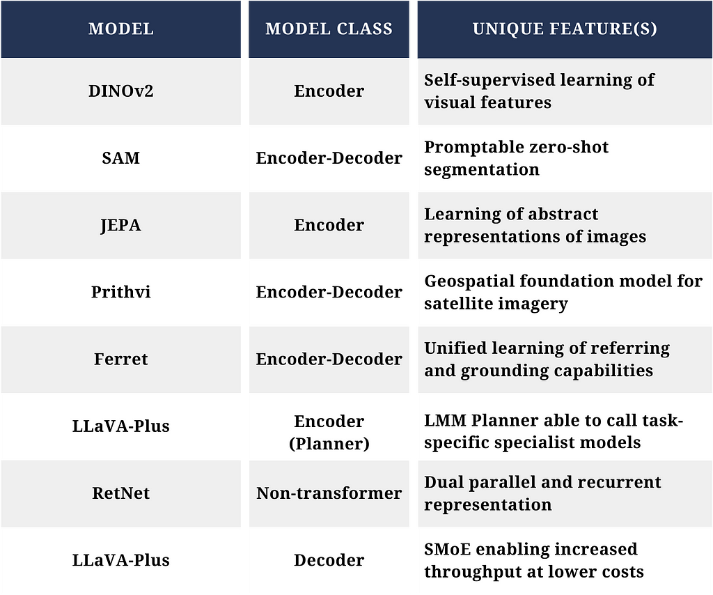
Although diverse and developed to accomplish different tasks, the models covered here illustrate the many innovation pathways that are being traversed in advancing AI capabilities. Of note, are the difference model classes (e.g., encoder only, encoder-decoder, decoder only) that are employed across the various models. A future effort may be to explore if there are performance benefits or tradeoffs due to class based on the task.
Characteristics of Select Surveyed Models
As these capabilities continue to mature, we will likely see a combining of features within models as certain features become expectations for performance. There will also be a shift towards creation of a multi-model ecosystem in recognition that one size does not fit all. Instead, AI agents acting as planners, orchestrators, and teammates will collaborate to dynamically select the best specialist model or tool for the task based on use case or Persona of Query driven needs [xxxii].
IV. Challenges and Risks
While the previous survey of model advancements helps illustrate the increasing rate of change within this field spurred by advancements in generative AI and foundation models, there are several challenges that cannot be overlooked as Federal organizations consider how to employ these capabilities. For the purposes of this section, we reference research primarily addressing LLMs. This was a deliberate choice to highlight risks inherent to models that leverage the autoregressive transformer architecture.
First, is the issue of resource constraints, both for enterprise training and inferencing of models and for model training and inferencing at the edge. The rise of ever larger AI models encompassing multiple billions of parameters is leading to strained resources due to infrastructure costs for compute, specialized AI talent needed to implement capabilities, and the challenges associated with amassing, curating, and training on the colossal data volumes required for such models. Such challenges can translate into financial shocks to organizational budgets that may have been set in the years prior due to the need to run high performance servers equipped with GPUs or attract and retain top AI talent. Additionally, there is an increasing need to perform training, retraining, and inferencing of models at the edge to support the processing, exploitation, and dissemination of detections of multimodal data. This requires the ability to run models on smaller hardware (e.g., human packable devices, onboard autonomous systems or sensors), where size, weight, and power are significant considerations.
The second of these is the issue of trustworthiness. To rely on generative AI and foundation models within mission critical workflows, one must be able to trust the output of such models. As such, the trustworthiness of models is of paramount concern. Much of the discourse on this topic has focused on hallucinations within the output, as well as attempts to define a broad set of dimensions against which to measure trustworthiness [xxxiii][xxxiv]. While these are valid concerns, trustworthiness extends beyond these dimensions to also include ensuring that the model arrives at the best possible outcome based on the latest corpus of data and training. One must be able to trust that the outcome is a global maximum in terms of suitability for the task, as opposed to a local maximum, which could have real world impacts if embedded into a mission critical workflow.
Third, and likely the most daunting, is that of security and privacy. To be able to leverage generative AI within Federal environments, one must be able to do so without compromise to the network and the data that resides on that network. Research has shown that LLMs can pose risks security and privacy and such vulnerabilities can be grouped into AI model inherent vulnerabilities (e.g., data poisoning backdoor attacks, training data extraction) and non-AI model inherent vulnerabilities (e.g., remote code execution, prompt injection, side channel attacks). To date, LLMs have been predominantly used in user level attacks such as disinformation, misinformation, and social engineering [xxxv], although new attacks continue to appear. For example, it has been shown that one can train deceptive LLMs able to switch their behavior from trusted to malicious in response to external events or triggers, eluding initial risk evaluation and creating a false sense of trust before attacking [xxxvi]. In addition, 2024 heralded the creation of AI worms [xxxvii] that can steal data and spread malware and spam. Such an attack uses an adversarial self-replicating prompt embedded within multimodal media files (e.g., text, image, audio) to effectively jailbreak and task the target LLM. Should future LLM/LMMs be given access to operating system and hardware-level functions, then threats from these vectors could escalate dramatically.
These challenges aren’t without opportunities. NIST recently released the inaugural version of its Artificial Intelligence Risk Management Framework [xxxviii] to aid with mitigating the risks related to AI. However, the nascent nature of this field means that much still remains unknown. Couple this with the fact that rigidity and bureaucracy within the RMF process means that, in some cases, by the time technology is approved for use and operationalized, it may be one or two generations behind state-of-the-art capabilities. Organizations face a challenge of how do they operationalize technology using a process that may take 9–12 months to complete when that same technology may be surpassed within six months.
V. Human-AI Collaboration: Redefining the Workforce
As AI trends continue to advance, this will have a profound impact on the dynamics of the workforce. Collaboration between humans and AI systems will become the norm as those who are able and willing to partner with AI will experience increased efficiency, innovation, and effectiveness. Supported by autonomous or semi-autonomous actions by AI agents [xxxix], human-AI teams will reshape how we make sense of and interact with the world.
AI will also play a pivotal role in transforming job roles and skill requirements. The workforce will need to adapt to this shift by acquiring new skills and competencies that complement, not compete with, AI’s capabilities and strengths. There will be a growing need for professionals who can effectively manage and collaborate with AI systems and other human-AI teams, increasing the demand for soft skills such as emotional intelligence, critical thinking, and creativity.
This evolution in skill sets will require changes in organizational talent programs to ensure training of the incoming workforce aligns to near-term and long-term organizational needs in AI. In addition to focusing on incoming professionals, organizations must prioritize upskilling and reskilling of the existing workforce to move the organization as a whole through the transformation journey to embrace this new AI era. While not covered in depth in this article, this topic is one that must be carefully considered to promote AI adoption in ways that take into account ethical considerations and ensure that AI systems are designed and implemented responsibly.
VI. Future Outlook and Recommendations
The pace of technological change will continue to accelerate over the next 18-month horizon. The precise path of this change is unpredictable, as each advancing month gives way to new developments that reframe the world’s understanding of the art of the possible. As breathtaking as some recent capabilities are, these technologies are still in a nascent stage. To have business and mission value, the maturation and commercialization of generative AI capabilities must continue, which will take some time.
In addition, Generative AI remains experimental and has not yet been operationalized for critical mission application. As organizations consider how to move forward with using the tremendous power of generative AI and foundation models, any strategy must be based upon a High OPTEMPO Concurrency where one is simultaneously experimenting with the newest technology, developing and training on a continuous basis in the mode of “Always in a State of Becoming” [xl]. To do so, organizations must be willing to accept additional risk, but also make use of emerging technologies to modernize existing methods. For example, LLMs have been shown to identify security vulnerabilities in code with greater effectiveness than leading commercial tools using traditional methods. Such methods can be used to enhance speed and efficacy in detecting vulnerable and malicious code as part of the RMF process [xli].
Posturing oneself to capitalize on AI advancements, especially in the realm of computer vision, necessitates that leaders within the organization become versed and remain current on rapidly progressing developments in AI. As part of their strategy, organizations should consider how to invest in the infrastructure and data foundation that will enable an AI-first future. This includes building modern data architectures and approaches to facilitate the rapid exchange of information as well as machine manipulation of data and services required to support automated discovery, understanding, and actions on the data. Moreover, organizations need to begin regular experimentation now in order to build the organizational capacity and learning needed for the future.
VII. Conclusion
As we progress through the remainder of the year, the trajectory of technological advancement is poised to surge into uncharted realms of what’s possible with AI. The advent of increasingly intricate multimodal models will revolutionize human-AI collaboration. Interactive analysis and interrogation of multimodal data, coupled with autonomous or semi-autonomous actions by AI agents and heightened reasoning capabilities derived from models able to create internal representations of the external world, will redefine operational landscapes.
The imperative to wield these capabilities to understand and decipher vast pools of visual and multimodal data, critical to national security, will define the latter half of this decade. Navigating this transformative era necessitates a forward-thinking mindset, the courage to increase one’s risk appetite, and the resilience to shape organizational strategy and policy to capitalize on the coming wave of change. As such, leaders must adopt a proactive stance in integrating AI, while placing an emphasis on its responsible deployment. Doing so will enable organizations to harness the full potential of evolving AI technologies.
All views expressed in this article are the personal views of the author.
References:
[i] S. Bubeck, V. Chandrasekaran, R. Eldan, J. Gehrke, E. Horvitz, E. Kamar, P. Lee, Y. Lee, Y. Li, S. Lundberg, H. Nori, H. Palangi, M. Ribeiro, Y. Zhang, “Sparks of Artificial General Intelligence: Early experiments with GPT-4,” arXiv:2303.12712, 2023. 13, 92
[ii] H. Naveed, A. Khan, S. Qiu, M. Saqib, S. Anwar, M. Usman, N. Akhtar, N. Barnes, A. Mian, “A Comprehensive Overview of Large Language Models,” arXiv:2307.06435, 2023. 1, 2, 3, 4
[iii] K. Pandya, M. Holia, “Automating Customer Service using LangChain: Building custom open-source GPT Chatbot for organizations,” arXiv:2310.05421, 2023. 1, 2
[iv] S. Pan, L. Luo, Y. Wang, C. Chen, J. Wang, X. Wu, “Unifying Large Language Models and Knowledge Graphs: A Roadmap,” arXiv:2306.08302, 2023. 1, 2
[v] Z. Xie, T. Cohn, J. Lau, “The Next Chapter: A Study of Large Language Models in Storytelling,” arXiv:2301.09790, 2023. 1, 2
[vi] Microsoft Research AI4Science, Microsoft Azure Quantum, “The Impact of Large Language Models on Scientific Discovery: a Preliminary Study using GPT-4,” arXiv:2311.07361, 2023. 4, 5
[vii] A. Shukla, L. Agarwal, J. Goh, G. Gao, R. Agarwal, “Catch Me If You Can: Identifying Fraudulent Physician Reviews with Large Language Models Using Generative Pre-Trained Transformers,” arXiv:2304.09948, 2023. 15, 16, 17
[viii] Z. Guo, S. Yu, “AuthentiGPT: Detecting Machine-Generated Text via Black-Box Language Models Denoising,” arXiv:2311.07700, 2023. 3, 4, 5
[ix] H. Xu, Y. Kim, A. Sharaf, H. Awadalla, “A Paradigm Shift in Machine Translation: Boosting Translation Performance of Large Language Models,” arXiv:2309.11674, 2023. 2, 3
[x] G. Savcisens, T. Eliassi-Rad, L. Hansen, L. Mortensen, L. Lilleholt, A. Rogers, I. Zettler, S. Lehmann, “Using Sequences of Life-events to Predict Human Lives,” arXiv:2306.03009, 2023. 3, 4, 5
[xi] K. O’Shea, R. Nash, “An Introduction to Convolutional Neural Networks,” arXiv:1511.08458, 2015. 3, 4, 5, 6, 7, 8
[xii] A. Dosovitskiy, L. Beyer, A. Kolesnikov, D. Weissenborn, X. Zhai, T. Unterthiner, M. Dehghani, M. Minderer, G. Heigold, S. Gelly, J. Uszkoreit, N. Houlsby, “An Image is Worth 16×16 Words: Transformers for Image Recognition at Scale,” arXiv:2010.11929, 2021. 2, 3, 4, 7, 8, 9
[xiii] M. Oquab, T. Darcet, T. Moutakanni, H. Vo, M. Szafraniec, V. Khalidov, P. Fernandez, D. Haziza, F. Massa, A. El-Nouby, M. Assran, N. Ballas, W. Galuba, R. Howes, P. Huang, S. Li, I. Misra, M. Rabbat, V. Sharma, G. Synnaeve, H. Xu, H. Jegou, J. Mairal, P. Labatut, A. Joulin, P. Bojanowski, “DINOv2: Learning Robust Visual Features without Supervision,” arXiv:2304.07193. 2023, 2, 4, 15, 20
[xiv] A. Kirillov, E. Mintun, N. Ravi, H. Mao, C. Rolland, L. Gustafson, T. Xiao, S. Whitehead, A. Berg, W. Lo, P. Dollár, R. Girshick, “Segment Anything,” arXiv:2304.02643. 2023, 5, 12
[xv] M. Assran, Q. Duval, I. Misra, P. Bojanowski, P. Vincent, M. Rabbat, Y. LeCun, N. Ballas, “Self-Supervised Learning from Images with a Joint-Embedding Predictive Architecture,” arXiv:2301.08243. 2023, 1, 2, 3, 4, 5, 6
[xvi] Y. LeCun, “A Path Towards Autonomous Machine Intelligence,” OpenReview.net. Version 0.9.2, 2022–06–27
[xvii] A. Dawid, Y. LeCun, “Introduction to Latent Variable Energy-Based Models: A Path Towards Autonomous Machine Intelligence,” arXiv:2306.02572. 2023, 8, 9, 10, 11, 12
[xviii] A. Bardes, Q. Garrido, J. Ponce, X. Chen, M. Rabbat, Y. LeCun, M. Assran, N. Ballas, “V-JEPA: Latent Video Prediction for Visual Representation Learning,” OpenReview.net. 2024–02–10
[xix] J. Jakubik, S. Roy, C. Phillips, P. Fraccaro, D. Godwin, B. Zadrozny, D. Szwarcman, C. Gomes, G. Nyirjesy, B. Edwards, D. Kimura, N. Simumba, L. Chu, S. Mukkavilli, D. Lambhate, K. Das, R. Bangalore, D. Oliveira, M. Muszynski, K. Ankur, M. Ramasubramanian, I. Gurung, S. Khallaghi, H. Li, M. Cecil, M. Ahmadi, F. Kordi, H. Alemohammad, M. Maskey, R. Ganti, K. Weldemariam, R. Ramachandran, “Foundation Models for Generalist Geospatial Artificial Intelligence,” arXiv:2310.18660. 2023, 2, 3, 4, 6, 21
[xx] K. He, X. Chen, S. Xie, Y. Li, P. Dollár, R. Girshick, “Masked Autoencoders Are Scalable Vision Learners,” arXiv:2111.06377. 2021, 3, 4
[xxi] R. Hamadi, “Large Language Models Meet Computer Vision: A Brief Survey,” arXiv:2311.16673. 2023, 4
[xxii] S. Yin, C. Fu, S. Zhao, K. Li, X. Sun, T. Xu, E. Chen, “A Survey on Multimodal Large Language Models,” arXiv:2306.13549. 2023, 5
[xxiii] D. Driess, F. Xia, M. Sajjadi, C. Lynch, A. Chowdhery, B. Ichter, A. Wahid, J. Tompson, Q. Vuong, T. Yu, W. Huang, Y. Chebotar, P. Sermanet, D. Duckworth, S. Levine, V. Vanhoucke, K. Hausman, M. Toussaint, K. Greff, A. Zeng, I. Mordatch, P. Florence, “PaLM-E: An Embodied Multimodal Language Model,” arXiv:2303.03378. 2023, 1, 2, 3, 6
[xxiv] S. Akter, Z. Yu, A. Muhamed, T. Ou, A. Bäuerle, Á. Cabrera, K. Dholakia, C. Xiong, G. Neubig, “An In-depth Look at Gemini’s Language Abilities,” arXiv:2312.11444. 2023, 2
[xxv] R. Girdhar, A. El-Nouby, Z. Liu, M. Singh, K. Alwala, A. Joulin, I. Misra, “ImageBind: One Embedding Space To Bind Them All,” arXiv:2305.05665. 2023, 1, 2, 3, 4
[xxvi] H. You, H. Zhang, Z. Gan, X. Du, B. Zhang, Z. Wang, L. Cao, S. Chang, Y. Yang, “Ferret: Refer and Ground Anything Anywhere at Any Granularity,” arXiv:2310.07704. 2023, 1, 2
[xxvii] S. Liu, H. Cheng, H. Liu, H. Zhang, F. Li, T. Ren, X. Zou, J. Yang, H. Su, J. Zhu, L. Zhang, J. Gao, C. Li, “LLaVA-Plus: Learning to Use Tools for Creating Multimodal Agents,” arXiv:2311.05437. 2023, 1, 2, 3, 4, 5, 6
[xxviii] H. Liu, C. Li, Q. Wu, Y. Lee, “Visual Instruction Tuning,” arXiv:2304.08485. 2023, 2, 3, 4, 5
[xxix] M. Minsky, Society of Mind, Simon and Schuster. 1988
[xxx] Y. Sun, L. Dong, S. Huang, S. Ma, Y. Xia, J. Xue, J. Wang, F. Wei, “Retentive Network: A Successor to Transformer for Large Language Models,” arXiv:2307.08621. 2023, 2, 3, 4, 5
[xxxi] A. Jiang, A. Sablayrolles, A. Roux, A. Mensch, B. Savary, C. Bamford, D. Chaplot, D. de las Casas, E. Hanna, F. Bressand, G. Lengyel, G. Bour, G. Lample, L. Lavaud, L. Saulnier, M. Lachaux, P. Stock, S. Subramanian, S. Yang, S. Antoniak, T. Le Scao, T. Gervet, T. Lavril, T. Wang, T. Lacroix, W. El Sayed, “Mixtral of Experts,” arXiv:2401.04088. 2024, 1, 2, 3
[xxxii] M. Zhuge, H. Liu, F. Faccio, D. Ashley, R. Csordás, A. Gopalakrishnan, A. Hamdi, H. Hammoud, V. Herrmann, K. Irie, L. Kirsch, B. Li, G. Li, S. Liu, J. Mai, P. Piękos, A. Ramesh, I. Schlag, W. Shi, A. Stanić, W. Wang, Y. Wang, M. Xu, D. Fan, B. Ghanem, J. Schmidhuber, “Mindstorms in Natural Language-Based Societies of Mind,” arXiv:2305.17066. 2023, 1, 2, 3, 4
[xxxiii] L. Sun, Y. Huang, H. Wang, S. Wu, Q. Zhang, C. Gao, Y. Huang, W. Lyu, Y. Zhang, X. Li, Z. Liu, Y. Liu, Y. Wang, Z. Zhang, B. Kailkhura, C. Xiong, C. Xiao, C. Li, E. Xing, F. Huang, H. Liu, H. Ji, H. Wang, H. Zhang, H. Yao, M. Kellis, M. Zitnik, M. Jiang, M. Bansal, J. Zou, J. Pei, J. Liu, J. Gao, J. Han, J. Zhao, J. Tang, J. Wang, J. Mitchell, K. Shu, K. Xu, K. Chang, L. He, L. Huang, M. Backes, N. Gong, P. Yu, P. Chen, Q. Gu, R. Xu, R. Ying, S. Ji, S. Jana, T. Chen, T. Liu, T. Zhou, W. Wang, X. Li, X. Zhang, X. Wang, X. Xie, X. Chen, X. Wang, Y. Liu, Y. Ye, Y. Cao, Y. Chen, Y. Zhao, “TrustLLM: Trustworthiness in Large Language Models,” arXiv:2401.05561. 2024, 6, 7
[xxxiv] Y. Liu, Y. Yao, J. Ton, X. Zhang, R. Guo, H. Cheng, Y. Klochkov, M. Taufiq, H. Li, “Trustworthy LLMs: a Survey and Guideline for Evaluating Large Language Models’ Alignment,” arXiv:2308.05374. 2023, 7, 8, 9
[xxxv] Y. Yao, J. Duan, K. Xu, Y. Cai, Z. Sun, Y. Zhang, “A Survey on Large Language Model (LLM) Security and Privacy: The Good, the Bad, and the Ugly,” arXiv:2312.02003. 2024 1, 2
[xxxvi] E. Hubinger, C. Denison, J. Mu, M. Lambert, M. Tong, M. MacDiarmid, T. Lanham, D. Ziegler, T. Maxwell, N. Cheng, A. Jermyn, A. Askell, A. Radhakrishnan, C. Anil, D. Duvenaud, D. Ganguli, F. Barez, J. Clark, K. Ndousse, K. Sachan, M. Sellitto, M. Sharma, N. DasSarma, R. Grosse, S. Kravec, Y. Bai, Z. Witten, M. Favaro, J. Brauner, H. Karnofsky, P. Christiano, S. Bowman, L. Graham, J. Kaplan, S. Mindermann, R. Greenblatt, B. Shlegeris, N. Schiefer, E. Perez, “Sleeper Agents: Training Deceptive LLMs that Persist Through Safety Training,” arXiv:2401.05566. 2024, 1, 2, 3, 4, 5, 6
[xxxix] J. Park, J. O’Brien, C. Cai, M. Morris, P. Liang, M. Bernstein, “Generative Agents: Interactive Simulacra of Human Behavior,” arXiv:2304.03442. 2023, 1, 2, 3
[xl] Concept referenced from Greg Porpora, IBM Distinguished Engineer on 21 February, 2024.
[xli] Y. Yao, J. Duan, K. Xu, Y. Cai, Z. Sun, Y. Zhang, “A Survey on Large Language Model (LLM) Security and Privacy: The Good, the Bad, and the Ugly,” arXiv:2312.02003. 2024 1, 2
In this beginner’s guide series on Object Detection models, we have so far covered the basics of object detection (part-I) and the R-CNN family of object detection models (part-II). We will now focus on some of the famous single-stage object detection models in this article. These models improve upon the speed of inference drastically over multi-stage detectors but fall short of the mAP and other detection metrics. Let’s get into the details for these models.
Single Shot Multi-box Detectors
The Single Shot Multibox Detector (SSD) architecture was presented by Liu et. al. back in 2016 as a highly performant single-stage object detection model. This paper presented a model which was as performant (mAP wise) as Faster R-CNN but faster by a good margin for both training and inference activities.
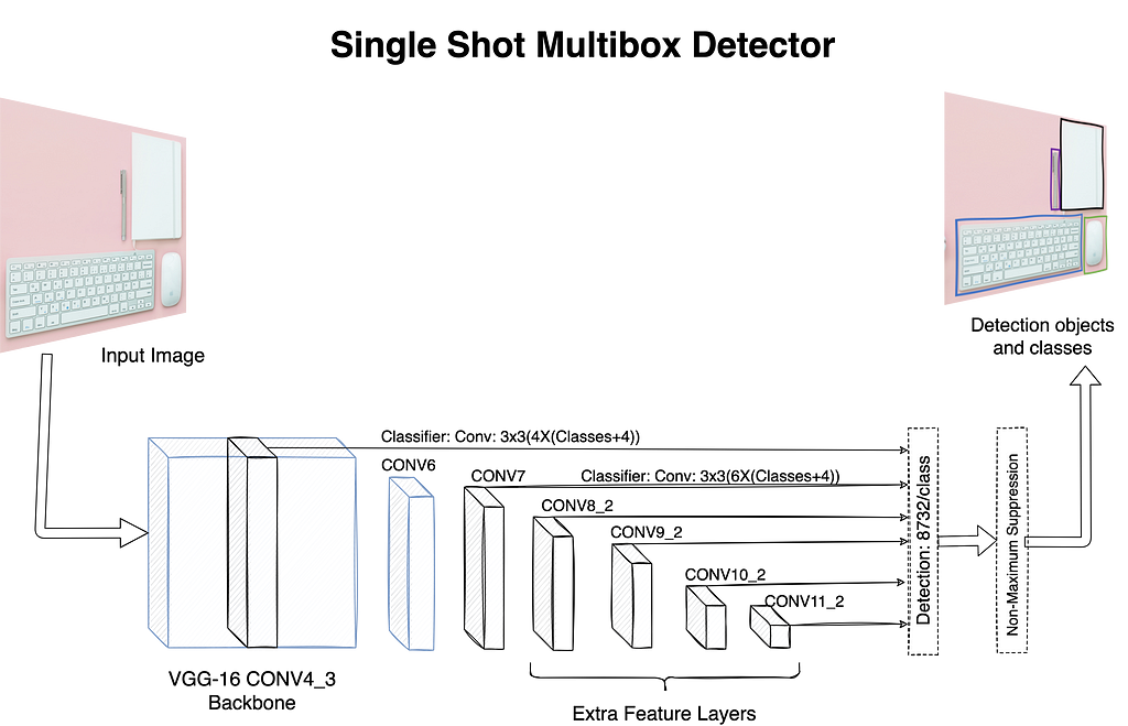
The main difference between the R-CNN family and SSDs is the missing region proposal component (RPN). The SSD family of models do not start from a selective search algorithm or an RPN to find ROIs. SSD takes a convolutional approach to work on this task of object detection. It produces a predefined number of bounding boxes and corresponding class scores as its final output. It starts off with a large pre-trained network such as VGG-16 which is truncated before any of the classification layers start. This is termed as the base-network in SSD terminology. The base-network is followed by a unique auxiliary structure to produce the required outputs. The following are the key components:
Multi-Scale Feature Maps: the auxiliary structure after the base-network is a sequence of convolutional layers. These layers progressively decrease the scale or resolution of feature maps. This comes in handy to detect objects of different size (relative to the image). The SSD network takes a convolutional approach to define class scores as well as relative offset values for the bounding boxes. For instance, the network uses a 3x3xp filter on a feature map of m x n x p, where p is the number of channels. The model produces an output for each cell of m x n where the filter is applied.
Default Anchor Boxes: The network makes use of a set of predefined anchor boxes (at different scales and aspect ratios). For a given feature map of size m x n, k number of such default anchor boxes are applied for each cell. These default anchor boxes are termed as priors in case of SSDs. For each prior in each cell, the model generates c class scores and 4 coordinates for the bounding boxes. Thus, in total for a feature map of size m x n the model generates a total of (c+4)kmn outputs. These outputs are generated from feature maps taken from different depths of the network which is the key to handle multiple sized objects in a single pass.
Figure 1 depicts the high-level architecture for SSD with the base-network as VGG-16 followed by auxiliary convolutional layers to assist with multi-scale feature maps.
Figure 1: High-level SSD architecture based on VGG-16. The architecture shows extra feature layers added to detect objects of different sizes. Source: Author
As shown in figure 1, the model generates a total of 8732 predictions which are then analyzed through Non-Maximum Suppression algorithm for finally getting one bounding box per identified object. In the paper, authors present performance metrics (FPS and mAP) for two variants, SSD-300 and SSD-512, where the number denotes the size of input image. Both variants are faster and equally performant (in terms of mAP) as compared to R-CNNs with SSD-300 achieving way more FPS as compared to SSD-512.
As we just discussed, SSD produces a very large number of outputs per feature map. This creates a huge imbalance between positive and negative classes (to ensure coverage, the number of false positives is very large). To handle this and a few other nuances, the authors detail techniques such as hard negative mining and data augmentation. I encourage readers to go through this well drafted paper for more details.
You Look only Once (YOLO)
In the year 2016, another popular single-stage object detection architecture was presented by Redmon et. al. in their paper titled “You Only Look Once: Unified, Real-time Object Detection”. This architecture came up around the same time as SSD but took a slightly different approach to tackle object detection using a single-stage model. Just like the R-CNN family, the YOLO class of models have also evolved over the years with subsequent versions improving upon the previous one. Let us first understand the key aspects of this work.
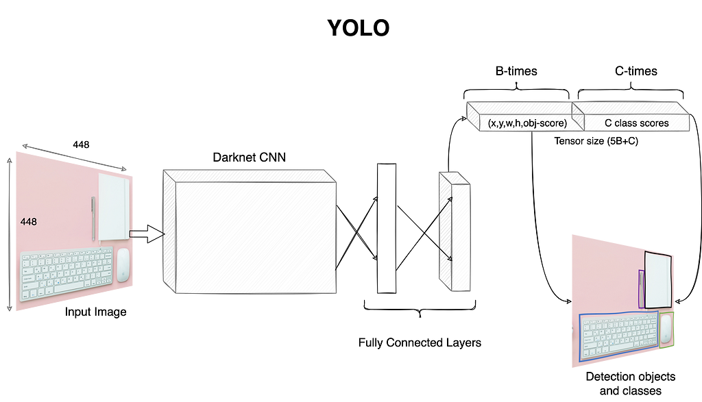
YOLO is inspired by the GoogleNet architecture for image classification. Similar to GoogleNet, YOLO uses 24 convolutional layers pre-trained on the ImageNet dataset. The pretrained network uses training images of size 224×224 but once trained, the model is used with rescaled inputs of size 448×448. This rescaling was done to ensure that the model picks up small and large objects without issues. It starts off by dividing the input image into an S x S grid (paper mentions a grid of 7×7 for PASCAL VOC dataset). Each cell in the grid predicts B bounding boxes, its objectness score along with confidence score for each of the classes. Thus, similar to SSD each cell in case YOLO outputs 4 coordinates of the bounding boxes plus one objectness score followed by C class prediction probabilities. In total, we get S x S x (Bx5 +C) outputs per input image. The number of output bounding boxes is extremely high, similar to SSDs. These are reduced to a single bounding box per object using NMS algorithm. Figure 2 depicts the overall YOLO setup.
Figure 2: High-level YOLO architecture which uses 24 convolutional layers followed by a few fully connected layers for final prediction. Source: Author
As shown in figure 2, the presence of fully connected layers in YOLO is in contrast with SSD, which is entirely convolutional in design. YOLO is built using an opensource framework called Darknet and boasts of 45FPS inference speed. Its speed comes at the cost of its detection accuracy. Particularly, YOLO has limitations when it comes to identification of smaller objects as well as cases where the objects are overlapping.
YOLOv2 or YOLO-9000 came the very next year (2017) with capability to detect 9000 objects (hence the name) at 45–90 frames per second! One of the minor changes they did was to add an additional step before simply rescaling the inputs to 448×448. Instead, the authors added an additional step where once the original classification model (with input size 224×224) is trained, they rescale the input to 448×448 and fine-tune for a bit more. This enables the model to adapt for larger resolution better and thus improve detection for smaller objects. Also, the convolutional model used is a 30-layer CNN. The second modification was to use anchor boxes and this implementation tries to get the size and number calculated based on the characteristics of the training data (this is in contrast to SSD which simply uses a predefined list of anchor boxes). The final change was to introduce multi-scale training, i.e. instead of just training for a given size the author trained the model at different resolutions to help the model learn features for different sized objects. The changes helped in improving model performance to a good extent (see paper for exact numbers and experiments).
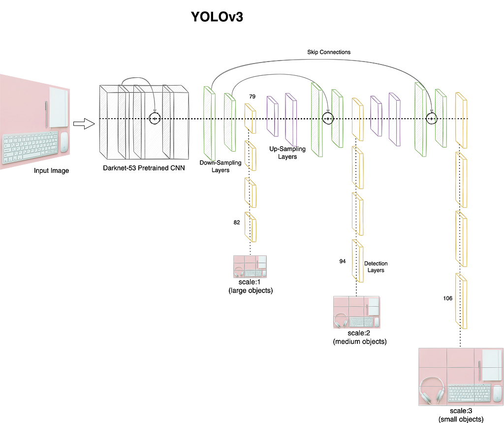
YOLOv3 was presented in 2018 to overcome the mAP shortfall of YOLOv2. This third iteration of the model used a deeper convolutional network with 53 layers as opposed to 24 in the initial version. Another 53 layers are stacked on top of the pre-trained model for detection task. It also uses residual blocks, skip-connections and up-sampling layers to improve performance in general (note that the time the first two version were released some of these concepts were still not commonly used). To better handle different sized objects, this version makes predictions at different depth of the network. The YOLOv3 architecture is depicted in figure 3 for reference.
Figure 3: YOLOv3 high-level architecture with Darknet-53 and multi-scale prediction branches. Source: Author
As shown in figure 3, the model branches off from layer 79 and makes predictions at layers 82, 94 and 106 at scales 13×13, 26×26 and 52×52 for large, medium and small sized objects respectively. The model uses 9 anchor boxes, 3 for each scale to handle different shapes as well. This in-turn increases the total number of predictions the model makes per object. The final step is application of NMS to reduce the output to just one bounding box per object detected. Another key change introduced with YOLOv3 was the use of sigmoid loss for class detection in place of softmax. This change helps in handling scenarios where we have overlapping objects.
While the original author of the YOLO model, Joseph Redmon, ceased his work on object detection[1], the overall computer vision community did not stop. There was a subsequent release called YOLOv4 in 2020 followed by another fork titled YOLOv5 a few weeks later (please note that there is no official paper/publication with details of this work). While there are open questions on whether these subsequent releases should carry the YOLO name, it is interesting to see the ideas being refined and carried forward. At the time of writing this article, YOLOv8 is already available for general use while YOLOv9 is pushing efficiencies and other benchmarks even further.
This concludes our brief on different object detection models, both multi-stage and single stage. We have covered key components and major contributions to better understand these models. There are a number of other implementations such as SPP-Net, RetinaNet, etc. which have a different take on the task of object detection. While different, the ideas still conform to the general framework we discussed in this series. In the next article, let us get our hands dirty with some object detection models.
From scaled approaches to more tailored ones — and why I think coaching from a distance is the future
Throughout my career, I ended up in multiple situations where I ran internal SQL trainings. While those training sessions were never a top priority for me — they are among the projects that gave me the most satisfaction. When you start seeing someone getting comfortable with running their queries, finding the information they need by themselves, building dashboards, and more generally getting excited by this newly acquired skill; I don’t know — it just feels good.
Recently, I saw the name of one of my former “students” popping up on a shared group to ask a pretty complex SQL question — and my reaction was the same as the one of Alfred when he nods to Bruce Wayne in “The Dark Knight Rises” (if you don’t have the reference — here it is).
The goal of this article is to walk you through my journey and my learnings on running internal SQL training to teach entire non-technical (or at least not SQL-savvy) teams, so hopefully you can share the gift of knowledge in your organization and get similar joy as I got.
Generally speaking, the situations that drove me to run these trainings fell into two broad categories:
Upskilling needs: Sometimes people in an organization can hit a ceiling because of their lack of SQL skills. A typical symptom of this is the apparition of convoluted processes that involve using multiple tools and spreadsheets to get to one final report. Granted, the solution is not always on the SQL side, but from experience, if you have one of those time-consuming multi-stage processes, and deep down you think that they’re got to be a better way to do what you are doing — most likely there is.
Resources scarcity: In an organization where analytical resources are scarce, I found it very beneficial (for both the organization and the individual) to identify individuals with “adjacent skills” (i.e. people who are used to working with spreadsheets and data) and to offer to upskill them. You end up broadening the horizon of an individual while generating more value for the business.
While there can be plenty of reasons why you’d want to run such a training (the above list is not exhaustive by any means; an argument could be made that this isn’t even mutually exclusive), it is important to be clear on what you want to achieve here. Depending on your goal, the way you’ll go about executing the training can differ greatly.
The early iterations, or how I discovered the limits of the “one size fits all” type of training
In my early iterations (back in 2015… dang, time flies!) I tried scaled approaches. The usual format was a typical classroom format: an X-week long program, with 1h weekly sessions (always at the same time on the same day), open to anyone interested in learning SQL, solely focused on SQL:
Every week, the group learned something new, starting from the “Hello World” of SQL (SELECT * FROM TABLE LIMIT 1) all the way to how to do window functions with multiple CTEs and optimizing queries.
Between each class, the group had to do some kind of homework (i.e. some exercises to test and solidify the knowledge they were learning in class)
While some people stuck to it to the end, the success rate (success being defined as when someone keeps using their newly acquired SQL skills post-training) was extremely low. Every session, fewer and fewer people were coming. Only a few people were doing the proposed exercises outside of class. Factually speaking, it wasn’t a success.
But I got a lot of good learnings from it:
I enjoyed mentoring: It taught me about the joy of mentoring and teaching new skills to others, which ultimately paved the way for this blog and other activities that I found generally rewarding.
There is a fear of SQL being “too technical”: A lot of people didn’t participate in those free trainings, or gave up at the very first obstacle, just because they considered SQL as something reserved for technical people, and they didn’t consider themselves as technical.
Having a training without a “retention” mechanism is bound to fail: It made me understand the importance of having some kind of system to keep people retained. Relying on people’s discipline for these kinds of training is wishful thinking — in any given organization, there are too many competing priorities and reasons to not complete this learning. So either you need to find students with strong intrinsic motivations for taking your training (e.g. you have a clear goal for learning SQL) or you need to provide them with strong extrinsic motivations (e.g. their managers expect them to learn SQL to take on some more technical projects).
Teaching SQL is just one part of the equation: Finally, and more importantly — it made me realize the importance of not teaching just SQL. Nobody uses SQL in a vacuum. The reality of SQL is that:
Before writing your SQL code, you need to locate the right datasets in your organization (which can be easy in mature organizations, but complicated in less mature ones, or even non-existent).
Once you have located the datasets, you need to locate the right fields for your query and make sure these fields contain the information you want / need (which is an art in itself)
From there, you need to request access to the dataset, and once you have access, you need to write the SQL code in a specific tool that has specific guidelines and features.
While writing your query, you need to keep an eye on computing cost, and potentially you need to re-factor things before running your query.
And so on and so on. If you don’t teach those elements as well, it will be hard for your students to use SQL.
All these learnings paved the way for the improved version of my program — a more tailored approach.
More recently — a shift toward a more tailored approach
After a couple of improved iterations of the above, I reflected on all the learnings I got along the way, and tried a new approach: I forgot about scale and went in the complete opposite direction. Instead of having 1h weekly sessions with a full class, I started having short weekly 1:1s with a few selected individuals.
While the program was still open to everyone, there was now a selection process to be a part of it. People who wanted “in” had to show the following:
Clear need for learning SQL: Prospective students had to fill in a form explaining why they wanted to learn SQL, and a project for which they needed SQL (e.g. “I want to automate X reporting, I want to build a dashboard on Y). If they were selected, this project would be the one they would work on for the whole duration of the program.
Pre-existing adjacent skills: Prospective students had to show what I call “adjacent skills”, i.e. skills that are similar to the skills you needed for SQL or data analysis in general.
Ability (and willingness) to carve enough time on their schedule: As part of their “application” to the program — students had to validate their “learning” project with their manager and be willing to dedicate at least X0% of their time over the next X weeks to learning. X0% might seem like a lot — truthfully it wasn’t really about the X0% — it was about sending a message (insert Joker meme). This program was going to be time-consuming and prospective students needed to make sure they could carve out the necessary time required to be successful.
On the training itself — the focus was shifted from SQL to doing a project. The first session of the training was spent on splitting their project into milestones. The very first milestone was kind of the same for everyone: find a resource (free or paid, online or offline — whatever they preferred) to learn the basics of SQL — and complete it.
I want to acknowledge this might be a bit disappointing — you would expect an article that is about “teaching SQL” not to be so dry on the “learning SQL” part. My general belief is that you can learn the key concepts of SQL in a very short amount of time but it will take you months/years to truly excel at it, and the sooner you start applying it to real-life problems, the faster you’ll get to a solid level. So the bulk of the program is spent on applying it to real-life problems, not on getting a basic understanding of SQL (that you can easily get on the amazing thing that is the internet).
Once the above first step was completed, we would start working toward the next milestones. For instance, for someone who would want to build a dashboard- we would split the project into:
Learning about the basics of SQL
Finding the right datasets and query logic (with learning how to get that information)
If necessary, building a database (with the roles and responsibilities tied to building a database)
Connecting this database to the dashboarding tool
Designing the dashboard
Building the dashboard
And from there, each student was supposed to reach a different milestone every week. They were always able to ping me or email me or have an office hour during the week if they were stuck somewhere, but generally speaking, they had to complete the milestones independently.
With this system, I saw a pretty high success rate (success being defined as when someone keeps using their newly acquired SQL skills post-training). And reflecting on it — I believe there are several reasons for this:
The selection process added friction: The added selection process made sure only the most motivated people with an actual project were part of the training.
The milestone system was a great forcing function: Having goals is a great start, but if there is no thought given to the steps needed to achieve the goal, and more generally to the work necessary to achieve the goal, there is little chance for the goal to be ever achieved. Having a milestone system, with clear deliverables under a clear deadline, creates an accountability and feedback loop that greatly helps the student grow.
Setting the right expectations from the beginning made everything simpler: I believe a big part of success in anything is linked to the mindset and our perception of the work. From the get-go with this program, I tried to set the right expectations: (1) It was going to be time-consuming (2) It was going to be challenging (3) It was going to be long
(4) But we were going to take the time, we were going to overcome the challenges one by one, and ultimately we were going to be victorious
Teaching people how to learn SQL by themselves vs actually teaching SQL: Last but not least — this key change made a huge difference in the program. It allowed them to become familiar with finding the key info they need on the web, experiment with it, and learn along the way. It made them way more independent, allowing them to keep growing, even after the program ended.
To date, the approach above is one of the most successful I have ever run. But it is pretty time-consuming, and I still see a lot of room for improvement.
Toward a more hybrid approach
At this point, the main question is:how might we scale the program above? If I reflect on the role I played in this training, it was mostly about giving direction and keeping people honest:
In the beginning: I helped students structure their projects and break them down into milestones
Before each milestone: I gave them some tips on the best way to approach each obstacle. If they get stuck, I gave them directionson how to unblock themselves.
Throughout the program: I celebrated their wins, challenged them, tried to keep them motivated when they were struggling, but also kept them accountable to deliver what they were supposed to deliver under the timeline they set.
I don’t think you can automate the above — or maybe you can with LLMs, who knows nowadays — but either way, you can definitely standardize it and optimize it, and maybe do a lot of that asynchronously, not necessitating a weekly meeting. And that’s what I would want to try for my next iteration — to reduce my time spent per student so that I can train larger cohorts.
Author’s note: I am seeing more and more fitness influencers offering “coaching from a distance”, where you can talk to your coach via email, send them videos about your training, and receive a personalized program. Maybe there is something similar to do for data analytics?
Regarding the program itself, I’d love to integrate some “community” elements. In particular, I am a strong believer in the Feynman technique — which is about (in a very simplified way) teaching what you learn. Concretely speaking, I’d want the students to start documenting their learnings and start sharing it back to new students (a bit like in the movie “Pay it Forward”). I see a couple of benefits here:
It could help scale the program (think of it as a “train the trainer” kind of approach) and allow more people to benefit from the knowledge
It would help “students” who are now teachers to internalize the key concepts they learned and identify gaps in their understanding
It would kickstart a huge knowledge base, that then can be used for more of a self-service approach for highly motivated individuals that might not be able to participate in the program
As always, ideas are cheap — execution is where you understand what works and what doesn’t — I am going to try to experiment with that shortly, and potentially report back in a future article.
In conclusion
Over the past 8 years, I tried different programs to turn colleagues and reports into SQL experts. I have not always been successful, but the pivot I made a couple of years ago from a wide-reaching program to a more tailored mentorship got me a lot of success and some great learnings.
My real challenge now is about the amplification of the method. How can we simplify and remove all the bullshit to focus on generating as much value as possible for the selected individuals, so that they are empowered to 10x the impact they are having in their organization? Maybe fitness influencers are onto something…
Hope you enjoyed reading this piece! Do you have any tips you’d want to share? Let everyone know in the comment section!
And If you want to read more of me, here are a few other articles you might like:
PS: This article was cross-posted to Analytics Explained, a newsletter where I distill what I learned at various analytical roles (from Singaporean startups to SF big tech), and answer reader questions about analytics, growth, and career.
We use cookies on our website to give you the most relevant experience by remembering your preferences and repeat visits. By clicking “Accept”, you consent to the use of ALL the cookies.
This website uses cookies to improve your experience while you navigate through the website. Out of these, the cookies that are categorized as necessary are stored on your browser as they are essential for the working of basic functionalities of the website. We also use third-party cookies that help us analyze and understand how you use this website. These cookies will be stored in your browser only with your consent. You also have the option to opt-out of these cookies. But opting out of some of these cookies may affect your browsing experience.
Necessary cookies are absolutely essential for the website to function properly. These cookies ensure basic functionalities and security features of the website, anonymously.
Cookie
Duration
Description
cookielawinfo-checkbox-analytics
11 months
This cookie is set by GDPR Cookie Consent plugin. The cookie is used to store the user consent for the cookies in the category "Analytics".
cookielawinfo-checkbox-functional
11 months
The cookie is set by GDPR cookie consent to record the user consent for the cookies in the category "Functional".
cookielawinfo-checkbox-necessary
11 months
This cookie is set by GDPR Cookie Consent plugin. The cookies is used to store the user consent for the cookies in the category "Necessary".
cookielawinfo-checkbox-others
11 months
This cookie is set by GDPR Cookie Consent plugin. The cookie is used to store the user consent for the cookies in the category "Other.
cookielawinfo-checkbox-performance
11 months
This cookie is set by GDPR Cookie Consent plugin. The cookie is used to store the user consent for the cookies in the category "Performance".
viewed_cookie_policy
11 months
The cookie is set by the GDPR Cookie Consent plugin and is used to store whether or not user has consented to the use of cookies. It does not store any personal data.
Functional cookies help to perform certain functionalities like sharing the content of the website on social media platforms, collect feedbacks, and other third-party features.
Performance cookies are used to understand and analyze the key performance indexes of the website which helps in delivering a better user experience for the visitors.
Analytical cookies are used to understand how visitors interact with the website. These cookies help provide information on metrics the number of visitors, bounce rate, traffic source, etc.
Advertisement cookies are used to provide visitors with relevant ads and marketing campaigns. These cookies track visitors across websites and collect information to provide customized ads.