Salinas de Janubio, Lanzarote, Canary Islands, Spain. Credit: imag3s 4 u
An introduction to panel data cross validation using PanelSplit
Motivation: As someone who works with panel data, I often need to perform cross validation. This involves training up to a certain point in time, testing on a subset of observations, training up to a further point in time, testing on a different subset of observations, and iteratively continuing this process on a panel data set. Sound familiar? This can be really frustrating to implement manually. To make things easier, I’ve created a package called PanelSplit that can help when working with panel data.
This article shows how you can use PanelSplit when working with panel data; from feature engineering, to hyper-parameter tuning, to generating predictions, PanelSplit is here to help!
What is panel data?
By panel data, I mean data where there are multiple entities over time. These entities could be countries, people, organizations, or any other unit of analysis. Multiple observations are recorded over time for these multiple entities.
What is cross validation?
Say we want to get estimates of how good our predictions are when we use a model. How can we do this? The standard approach is cross validation, which involves splitting the data up into successive folds, each with its unique training and testing set. The visualization below shows what this looks like for time series data.
An example of time series cross validation.
While there is already a scikit-learn function to do time series cross validation called TimeSeriesSplit, it doesn’t work with panel data. Rather than being a single time series for one entity, panel data has multiple entities and we need a tool that allows us to work with multiple entities.
This is where PanelSplit comes in. PanelSplit is a package that allows us to generalize TimeSeriesSplit to panel data. It also offers functionality for transforming, predicting, and much more, but in this introductory article I’ll cover the just basics.
Performing cross validation with PanelSplit
Now that we’ve introduced what panel data is and what cross validation looks like in this setting, let’s see how to do cross validation using PanelSplit.
First, let’s generate some example data to work with:
import pandas as pd
import numpy as np

# generate example data
num_countries = 3
years = range(2000, 2005)
num_years = len(years)

data = {
    'country_id': [c for c in range(1, num_countries + 1) for _ in years],
    'year': [year for _ in range(num_countries) for year in years],
    'y': np.random.normal(0, 1, num_countries * num_years),
    'x1': np.random.normal(0, 1, num_countries * num_years),
    'x2': np.random.normal(0, 1, num_countries * num_years)
}

panel_data = pd.DataFrame(data)

# display the generated panel data
display(panel_data)
The generated panel data. There are 3 countries observed from 2001–2004.
After generating our panel data set, we can now apply PanelSplit.
Initializing PanelSplit
When we initialize PanelSplit, we define the cross validation approach that we are going to use.
The periods argument takes the time series. In this case the series is the year column.
n_splits, gap, and test_size are all arguments used by TimeSeriesSplit to split up the time series.
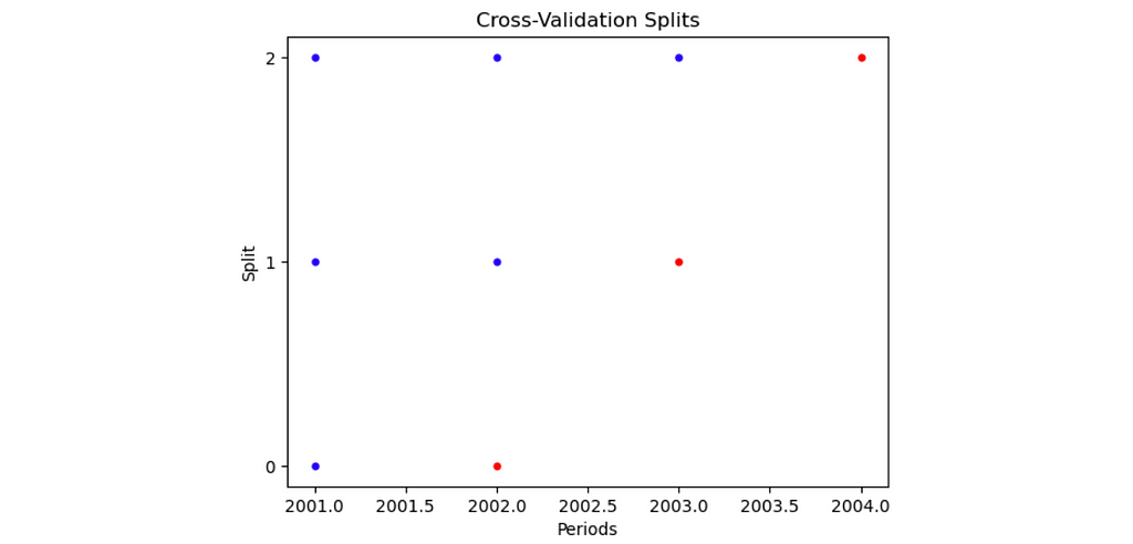
By specifying plot=True, a visualization is produced describing the train and test sets within each split.
!pip install panelsplit from panelsplit import PanelSplit
The output of initializing PanelSplit when plot = True. Based on the arguments we provided, there are 3 splits, there is no gap between train and test sets, and the test size is one period for each split.
Understanding how PanelSplit works
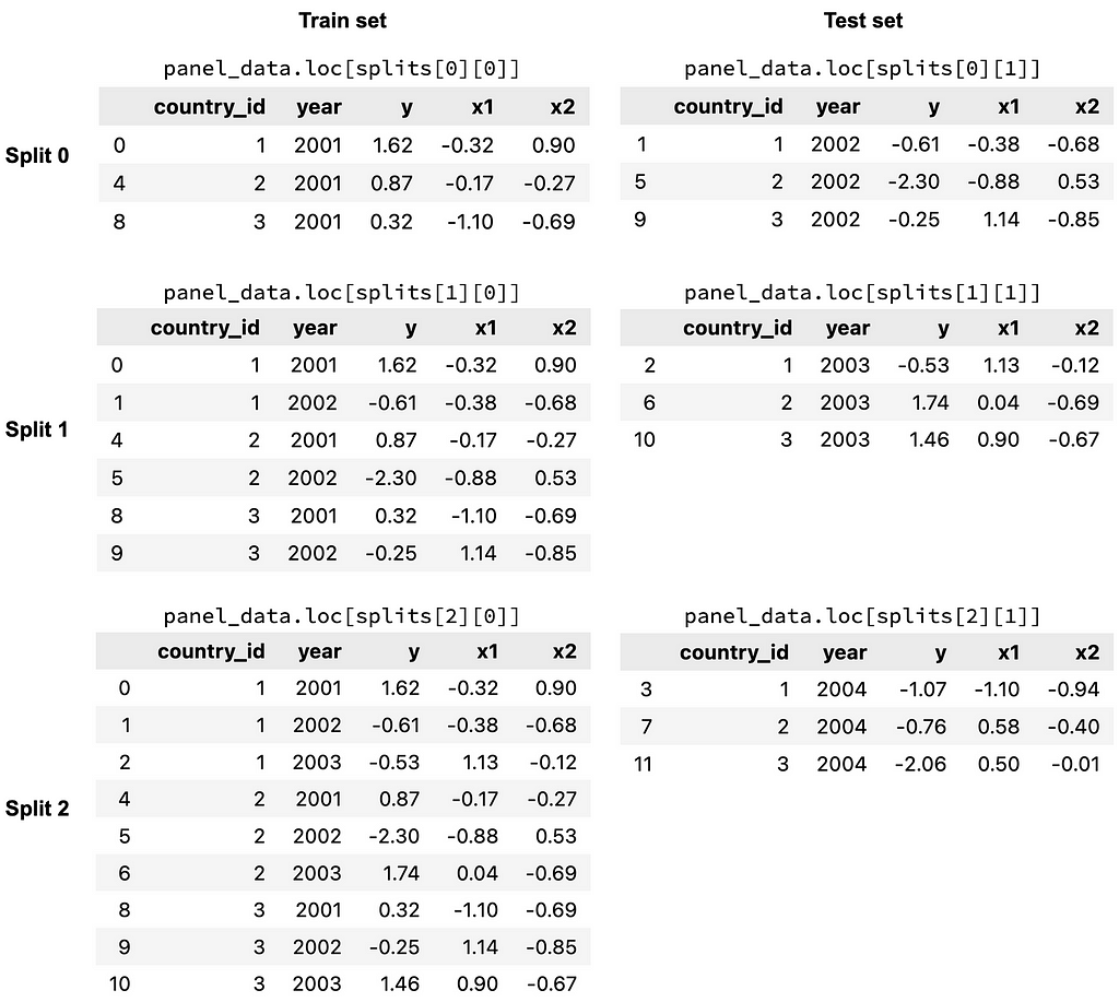
To get a better idea of what the splits look like, let’s use the split() function to return the different train and test sets for each split.
splits = panel_split.split()
The splits object contains the 3 splits of the cross validation procedure. Within each split, there is a list, which consists of the train indices (the first item) and test indices (the second item). The indices are True and False values, indicating whether or not a row is in a particular train/test set for a particular split. These indices can be used to filter for different subsets of the data, as shown in the figure below.
Demonstration of the different train and test sets within each split.
Hyper-parameter tuning
Now that we’ve created an instance of PanelSplit, let’s do some hyper-parameter tuning!
Here we do a basic hyper-parameter search with a Ridge model, specifying the cv argument for GridSearchCV to be panel_split. During GridSearchCV’s fit procedure it calls panel_split’s split() function, returing the indices for each train and test for each split. It uses these indices to filter the data that are provided as the X and y arguments in the fit() function.
from sklearn.linear_model import Ridge
from sklearn.model_selection import GridSearchCV

param_grid = {'alpha':[.1, .5]} # define the hyper-parameter grid space

# define the gridsearch and call fit, specifying panel_split for the cv argument
gridsearch = GridSearchCV(estimator = Ridge(), param_grid=param_grid, cv=panel_split)
gridsearch.fit(X = panel_data[['x1','x2']], y = panel_data['y'])

print(gridsearch.best_params_)
In this search, the optimal alpha for the Ridge model is .5.
Hooray! We’ve found the optimal set of hyper-parameters. Now we can use these to predict.
Note: In a real setting we’d differentiate between the test set used for hyper-parameter tuning and the test set used for evaluating performance, but for this example let’s keep the validation set and the test set the same.
Generating predictions with cross_val_fit_predict
Generating predictions is really easy with PanelSplit.
Using cross_val_fit_predict, we specify that we want to use our best Ridge model, our X and y, and PanelSplit will fit on each training set and predict on each test set, for each split.
predictions, models = panel_split.cross_val_fit_predict(estimator = Ridge(gridsearch.best_params_),
                                                   X = panel_data[['x1','x2']],
                                                   y = panel_data['y'])
The predictions as well as the fitted models are returned. If we want to include the identifiers for the predictions, we can generate labels using gen_test_labels and then create a new Pandas Series in our predictions_df DataFrame.
This is just a basic demo, but PanelSplit can do so much more! For example:
With cross_val_fit_transform we can fit on training sets and transform on test sets. If we have missing features that need imputation this is really helpful.
What if we want to scale the data and each split needs its own ‘snapshot’ of the data in order to keep the scaling transformations separate? We can use gen_snapshots to do this! Or use a scikit-learn pipeline as the estimator in cross_val_fit_predict 🙂
What if we are missing a time period? By using the unique periods argumentwith the drop_splits argument upon initialization, PanelSplit can handle this and drops splits where there aren’t any observations.
If you’re looking to see some more examples and want to try PanelSplit out for yourself, check out the Jupyter notebook I created where I cover some additional capabilities.
This is the first package I have written, so I learned a lot working on this project. Thank you for reading, and I hope PanelSplit helps you in your next panel data project!
Note: Unless otherwise noted, all images are by the author.
The ability to predict the future is a superpower!
Fortunately, Time Series Forecasting exists and is accessible to anyone and everyone! This superpower can enable anyone to make proactive decisions and improve their planning for the future. The applications of time series forecasting are endless; think about being able to predict the demand for a product in your business, make more informed financial decisions on your investments or simply being able to forecast the weather.
While the internet overflows with resources covering the core principles of forecasting, the real-world complexities often go beyond textbook lessons. This guide delves into the unspoken secrets I’ve discovered through my years of applying this powerful tool in business settings. We will explore various strategies that go beyond the typical focus on feature engineering and model selection to help you truly unlock the potential of Time Series Forecasting.
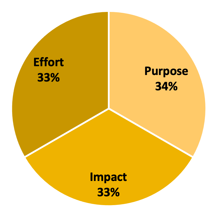
The first key step in any Data Science project is to always to look at the Purpose, Impact, and Effort associated with their work. Before heading into the complex world of data analysis and modelling, it’s important to pause and evaluate the fundamental questions: What is the purpose of this endeavour? What impact will it ultimately have? And is it worth the effort?
Data science projects often require alot of time and resources. Therefore, the crucial question you must continuously ask yourself is “How much additional value does the organization gain by utilising data science?”
Surprisingly, the answer to this question is not always straightforward. Sometimes, choosing a ‘quick and dirty’ solution — in line with the Pareto Principle, where 20% of the effort yields 80% of the results — solves most everyday problems, so why spend the extra time and effort if a simpler solution can suffice?
This is where the PIE framework comes into play. Beyond the incredibly exciting data science techniques lies an important decision: Is the marginal benefit of using more advanced techniques really worth the additional cost and effort? In most cases, the answer is a resounding “no.”
As exciting as it may seem, it’s important to think critically about any data science project before jumping straight in. By following the PIE framework, you can confidently decide on the right projects to undertake ensuring that your efforts are both meaningful and impactful.
Pie chart on the PIE Framework.
2.Domain Knowledge
Many courses and textbooks usually focus on teaching various time series forecasting techniques, often presenting them as the key ingredient for success. However, as experience has taught me in the real world, the real “secret weapon” is not in the model itself, but deeply understanding the data you’re working with. There is no one-size-fits-all forecasting model.
For example, imagine trying to build your dream house on a foundation of loose sand. You can approach the best architects and builders, and create the most intricate blueprint, but ultimately the house is destined for disaster. Similarly, building a robust forecasting model with irrelevant data or riddled with errors and inconsistencies is like building on unstable ground. The model’s outputs will be unreliable and prone to collapse.
Domain knowledge, in the context of time series forecasting, is more than just knowing what the data represents. It’s about digging in deeply and understanding the underlying relationships, mechanisms, and nuances specific to the problem you’re analysing. Each dataset is unique and your investigation into understanding the data will vary with every project.
While this step can seem quite boring, it can make or break the entire project. From informing feature engineering decisions to guiding model selection, domain knowledge plays a very important role in shaping the project. If you’re able to find and utilise the best data to feed into the model, your output would be considerably more useful.
3.Non-Stationarity and Sudden Shifts
When you first learn about Time Series forecasting, you’ll often encounter the core assumption of “Stationarity” in lots of forecasting models. However, in the real world, Time series data rarely conforms to this assumption. Instead, you’ll find that the data and interactions change over time. This is usually characterized by fluctuations, trends, and seasonality. When building a reliable forecasting model, it is important to identify and accommodate these dynamic patterns to accurately capture and predict the underlying trends and behaviour.
Another common problem is when sudden shifts or discontinuities occur in the data. Traditional forecasting methods don’t handle these sorts of shifts very well, but it is important to take these into consideration. These breaks can be a result of external factors ranging from changes in market conditions, shifts in consumer behaviour, or the introduction of new regulations or technologies. They may not always be directly measurable or available, but this is where your expertise would come into play here in finding the best way to account for these nuances.
For example, imagine you’re trying to predict the number of viewers of the English Premier League football. Apart from the obvious on/off-season, there are a few other quirks that happen, such as a high seasonal effect towards the end of the season where the stakes are higher, and viewers become more interested. Now imagine Messi moves to the Premier League or Sky Sports increase their monthly subscription fee — these sudden shifts are sometimes unpredictable but impacts the actual viewership quite significantly.
There’s no easy way to handle these shifts, but there are techniques that can help. Here are a few approaches that I typically use to address these nuances, but the application of them is highly dependent on the nature of the data;
1. Time series decomposition — This involves separating the data into its core components — such as trend, seasonality, and noise. This step should typically be done as part of the pre-analysis to better understand the data and model each component’s behaviour individually.
2. Exogenous features — These are the external variables that you think affect the short-term volatility or the long-term trends of the data. This can be manual flags or the other important features to use as regressors. Domain Knowledge is crucial here. For each sudden shift, there is usually an explanation. It’s not always possible to incorporate each explanation as a feature, so it’s important to filter through the most useful, reliable, and predictable ones to avoid overfitting.
3. Adaptive Modelling — This involves selecting the most appropriate model that can detect and adapt to shifts in the underlying patterns. This step is one of my favourites as it involves research in finding or creating the best model for the data. However, it’s easier said than done. There may be times where this may involve some manual work, such as hyperparameter tuning or utilising a specific model that considers certain nuances of the data. Keep in mind that this may also increase the risk of overfitting.
While these techniques can’t perfectly predict every unprecedented effect, they do prepare us more for them and build more robust forecasting models.
4.Stakeholder Management
Successful implementation of a model goes far beyond the technical intricacies of model selection and data analysis — it encompasses effective stakeholder management. Think of ‘Stakeholder Management’ as tailoring the process to the people involved. The goal is to ensure that your model is doing what it needs to do, and you continue to bring value. How you tailor the process and output depends on the needs of the stakeholders, whether this is executives, managers or consumers. It’s all about delivering actionable insights that enable them to make informed decisions.
As a data scientist, your worth is often determined by how well you translate your technical insights into real-world decision-making. This is both a blessing and a curse to most of us — soft skills are notoriously undervalued in technical fields, but acts as the bridge between our mind-crunching work and the value than can be derived from it. While technical skills are important for the foundation for our work, your ability to communicate effectively, empathize with stakeholders, and drive action is what truly elevates our impact. Communication is the single most important skill as a data scientist, yet it is stereotypically also the most difficult to acquire.
Below are some actionable tips that can help in effective communication:
1. Tailoring model selection
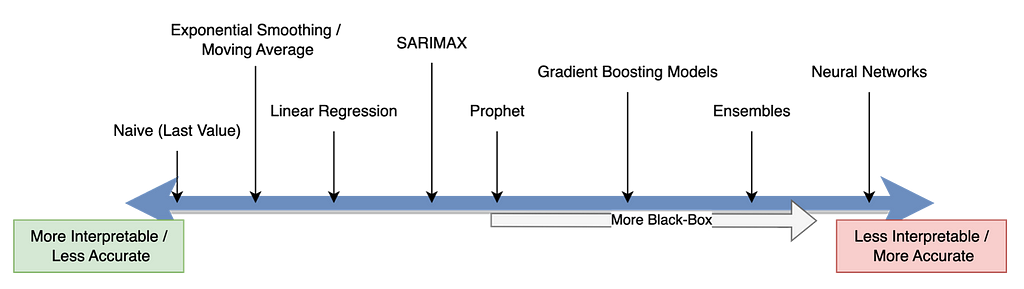
Choosing the right model goes far beyond identifying the most accurate algorithm.
It’s true that black-box models can be the most accurate and engaging for us Data Scientists, but they’re often not transparent or easily interpretable, making it hard for stakeholders to trust the results. This is where it may be better to opt for simpler models like ARIMA or Exponential Smoothing where you may decrease accuracy but increase interpretability. It is always best to do research on the various models that exist.
Here’s an example of some of the most common forecasting models and their interpretability;
2. Clear Visualisations
Present your results in a way that resonates with your audience.
Think about well-designed charts, graphs, and dashboards. This involves clarity, simplicity, and relevance to the audience. How can you help stakeholders grasp key insights quickly and make informed decisions?
There are numerous articles and courses online that help in data visualisation!
Executives might favour high-level dashboards, while managers might require detailed reports with error metrics. Consumers typically benefit from clear and actionable visualizations that translate forecasts into practical applications.
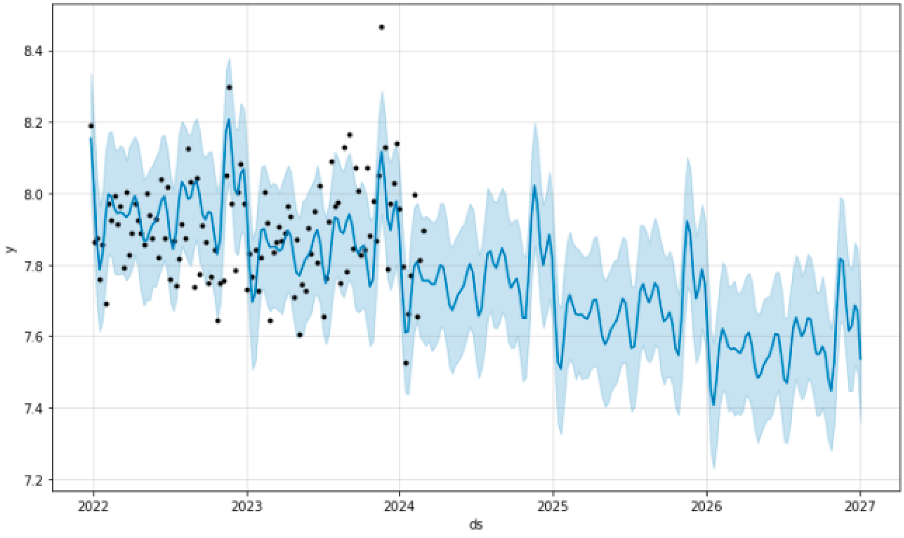
Personally, I take a lot of inspiration from Prophet’s base visualisations as it clearly depicts the actual values vs the model predictions. I usually add annotations or highlight certain points (both future and past) for significant moments.
Example of Prophet output.
3. Storytelling
Don’t just present data; tell a story. Highlight the context, key findings, and potential implications of your forecasts. Understand your audience and frame the narrative in a way that is relevant to the specific goals and challenges.
Focus on the “Why” before the “How”
What is the overall objective you’re trying to achieve with the forecast
How will the forecasts be used to inform decision-making?
What are the potential consequences of inaccurate forecasts?
Acknowledge the limitations and uncertainties in the model’s predictions
Highlight the Journey, not just the Destination
Always tie in the journey to the main task at hand.
Share key challenges you encountered during data pre-processing or model selection and how you overcame them.
Highlight any unexpected insights you discovered along the way.
Make it Relatable and Actionable
Speak the language of your audience.
Quantify the potential impact of your forecasts on metrics like revenue, cost savings, or resource allocation.
Offer clear recommendations and actionable steps stakeholders can take based on your insights.
Remember, the key to successful forecasting goes far beyond the accuracy of the model, to its ability to empower stakeholders to make informed decisions. Time-series forecasting is a powerful tool, so use it wisely and carefully!
Unless otherwise noted, all images are by the author.
This post was created in collaboration with Max Rabin.
This is the second part of a series of posts on the topic of maximizing the utility of scarce AI resources. In the first post we noted the increasing limitations on the ability to scale up AI resources at will and, as a consequence, the growing trend of AI development teams to guarantee AI compute capacity by means such as building up an in-house AI server farm and/or reserving dedicated instances in the cloud. The scarcity of AI compute resources motivates the design of specialized scheduling solutions to minimize idle time and prioritize critical workloads. Please see our previous post in which we proposed a detailed list of requirements for such solutions. The approach we took there was to leverage the existing priority-based scheduler that comes with Kubernetes and align our training development workflow to its use. In this post we explore the option of maintaining our existing framework for training AI models and enhancing it with our own custom implementation of a priority-based scheduler. Importantly, the need for this type of solution is often motivated not just by the scarcity of AI resources, but also by the desire to increase control over the orchestration and prioritization of training workloads so as to reduce development costs. For example, even in a scenario of abundant capacity, you may choose to limit your use to a fixed number of training instances so as to cap your training expenditure.
For the purposes of this post, we will assume that our training framework of choice is AWS’s managed service for AI model training, Amazon SageMaker. The solution we will propose will use additional AWS services such as Amazon DynamoDB and AWS Lambda. The choice to demonstrate our solution using AWS services should not be viewed as endorsement. There are many cloud-based service offerings available and the best one for you will depend on the particular details of your project. Similar solutions to the one that we will describe can be designed on other cloud-based environments and/or using alternative cloud-based services.
The Traditional Method for Starting Up SageMaker Training Jobs
Traditionally, we would start up a SageMaker training job using the Amazon SageMaker Python SDK. In the code block below we use the SageMaker SDK (version 2.208) to run a PyTorch training workload on a single instance of type p5.48xlarge.
When the estimator.fit() function is called, the SageMaker library uploads our code to Amazon S3 and then transforms the request to a boto3 SageMaker client create_training_job request (see here).
This method for starting up training jobs is dependent on the availability of the requested resources for its success. In our scenario of scarce AI resources, it is likely to fail more often than not. Although this can be partially mitigated by retaining provisioned compute instances for successive workloads, the API does not provide the appropriate tooling for maximizing their utility. Let’s suppose that we wish to utilize precisely two p5.48xlarge instances. To simplify our discussion, let’s assume that each training workload runs on a single instance. Typically, during an AI model development cycle there will be periods when there are more than two training workloads that are waiting to be processed. The existing API would try to start up a third p5.48xlarge instance and would most likely fail due to its limited availability. Even when there is instance availability, we may wish to limit our training to just our two designated instances to increase our control over the costs of training.
We require a new API for submitting jobs for training, one that does not immediately start up a new p5.48xlarge instance, but rather enters the jobs to a priority queue. And we need an associated job scheduler that manages the use of our two resources while prioritizing critical workloads.
Importantly, please note that as of the time of this writing, Amazon SageMaker does not support the option of training on reserved Amazon EC2 instances. And although Amazon SageMaker Savings Plans has similar properties to instance reservations, it does not guarantee instance capacity. In a previous post we addressed this limitation and proposed using SageMaker managed warm pools as an alternative method for retaining access to provisioned instances. For the remainder of the post, we will assume that we are able to attain two instances of our choice whether it be through this or some other method.
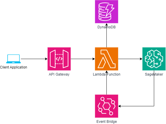
We start by using Amazon API Gateway to define a private REST API for submitting training job requests. We name the API training-job-queue. Later, we will add a POST method called add-job and modify our training-job creation code to use this method instead of the SageMaker client create_training_job API. The code block below contains the definition of the private API resource in SAM. In practice you will likely want to specify access limitations to the API and/or a method of authorization.
We define a function that creates a table entry from a given training job request. We assume that request contains the same contents as the input to the create_training_job API in JSON format. We further assume that the priority of the workload is entered as a key-value tag in the training job definition.
The REST API add-job method that we will soon define will be programmed to call the add_job_entry function.
We define a second function that extracts the pending jobs from the database and returns them in order of priority. In the case that multiple jobs have the same priority, they are ordered according to the amount of time they have been waiting in the queue.
from boto3.dynamodb.conditions import Attr

# Get a list of all pending jobs sorted by priority
def get_pending_jobs():
    response = table.scan(
        ProjectionExpression='jobName, priority, entryTime',
        FilterExpression=Attr('jobState').ne('running')
    )
    jobs = response.get('Items', [])

    # sort jobs, first by priority (descending) and then by entryTime
    sorted_jobs = sorted(jobs,
                         key=lambda x: (-x['priority'], x['entryTime']))

    return sorted_jobs
The following utility functions will come in handy in the next sections.
# Get a jobName -> priority mapping of all running jobs def get_running_jobs_dict(): # Get all running jobs response = table.scan( ProjectionExpression="jobName, priority", FilterExpression=Attr('jobState').eq('running') ) jobs = response.get('Items', [])
running_jobs = {job['jobName']: job['priority'] for job in jobs}
return running_jobs
# Print the queue state def print_queue_state(): response = table.scan( ProjectionExpression='jobName, jobState, priority' ) jobs = response.get('Items', [])
print_table = [] for job in jobs: print_table.append([job['jobName'], job['jobState'], job['priority']])
# sort by priority sorted_table = sorted(print_table, key=lambda x: -x[2]) # Print the table from tabulate import tabulate print(tabulate(sorted_table, headers=['Job Name', 'State', 'Priority']))
# get job state or None if the job does not exist def get_job_state(job_name): response = table.get_item( Key={'jobName': job_name}, ProjectionExpression='jobState' ) job = response.get('Item') return job.get('jobState') if job else None
# update the job state def update_job_state(job_name, new_state): table.update_item( Key={'jobName': job_name}, UpdateExpression="SET jobState = :new_state", ExpressionAttributeValues={":new_state": new_state} ) print(f'Update job {job_name} to {new_state}')
# remove a job entry def remove_job(job_name): table.delete_item( Key={'jobName': job_name} ) print(f'Removed job {job_name} from queue')
Both our choice of DynamoDB and its usage (e.g., our use of the Scan API rather than the Query API) assume that the overall number of jobs in our queue will be in the dozens, at most. For a larger scale solution, you may be better off with a heavier duty database (e.g., one that performs the sorting operation for you) or a more sophisticated use of DynamoDB (e.g., see here).
Define the Training Job Queue Manager
The main component of our solution is the training job scheduler. Here we implement a rather simple manager that performs the following steps:
Extract the list of queued jobs, ordered by priority. If none exist, return.
Discover unused instance capacity. For each free instance, start one pending job on SageMaker. If no jobs remain after that, return.
Calculate the number of SageMaker jobs in the Stopping state. If greater than the number of pending jobs, return.
Assess the need for preemption of running SageMaker jobs by comparing their priorities to those of our pending jobs.
# set the limit on total number of instances/jobs
MAX_CAPACITY = 2

sagemaker = boto3.client('sagemaker')

# apply a queue stamp to identify that the job came from the queue
def apply_qstamp(job_name):
    return f'{job_name}-qstamp-{datetime.now().strftime("%d%H%M")}'

# strip the queue stamp
def strip_qstamp(job_name):
    return job_name.split('-qstamp-')[0]

# start a SageMaker job and update job entry in queue
def start_job(job_name):
    print(f'start job {job_name}')
    job_details = get_job_details(job_name)
    job_details['TrainingJobName'] = apply_qstamp(job_name)
    if(job_details):
        # start job with detail from queue
        # (you may optinally overwrite fields such as the iam role)
        response = sagemaker.create_training_job(**job_details)
        if response['ResponseMetadata']['HTTPStatusCode'] == 200:
            print(f'started job {job_name}')
            update_job_state(job_name, 'running')

# preempt a SageMaker job and update job entry in queue
def preempt_job(job_name):
    print(f'preempt job {job_name}')
    response = sagemaker.stop_training_job(TrainingJobName=job_name)
    if response['ResponseMetadata']['HTTPStatusCode'] == 200:
        print(f'preempted job {job_name}')
        update_job_state(strip_qstamp(job_name), 'preempted')

# get SageMaker jobs
def get_sagemaker_jobs(status):
    running = sagemaker.list_training_jobs(StatusEquals=status)
    return running.get('TrainingJobSummaries', [])

# queue manager
def manage_queue():
    # extract pending jobs to run
    pending = get_pending_jobs()

    if not pending:
        return

    if len(pending) > MAX_CAPACITY:
        pending = pending[:MAX_CAPACITY]

    # get running sagemaker jobs
    running = get_sagemaker_jobs('InProgress')
    total_running = len(running)

    # get stopping sagemaker jobs
    stopping = get_sagemaker_jobs('Stopping')
    total_stopping = len(stopping)

    # calculate the number of free instances
    free_slots = MAX_CAPACITY - total_running - total_stopping

    jobs_to_start = min(len(pending), free_slots)

    # for each free instance, start a job
    for i in range(jobs_to_start):
        start_job(pending[i].get('jobName'))

    still_pending = pending[jobs_to_start:]

    if not still_pending:
        return

    # assume that 'total_stopping' number of jobs will start soon
    test_for_preemption = len(still_pending) - total_stopping
    if test_for_preemption <= 0:
        return

    # check if preemption is required
    test_priority = still_pending[total_stopping:]

    running_jobs = get_running_jobs_dict()
    priority_dict = {}
    for job in running:
        job_name = job['TrainingJobName']
        priority_dict[job_name] = running_jobs[strip_qstamp(job_name)]

    # sort running jobs from lowest to highest priority
    sorted_running = sorted(priority_dict.items(), key=lambda item: item[1])

    index = 0
    while index < test_for_preemption and
          test_priority[index].get('priority') > sorted_running[index][1]:
        preempt_job(sorted_running[index][0])
        index = index + 1
Important notes:
Our implementation is highly optimistic in the sense that we assume that all the jobs that are inserted are valid and that we will be able to start them up on SageMaker without issue. In practice, appropriate error handling should be added (e.g., removing faulty jobs from the queue with appropriate logging).
In a production environment, we would need to take into consideration the likely occurrence of a race condition when our queue_manager is triggered by multiple concurrent events. There are several ways of addressing this problem (e.g., see here) including enforcing atomicity (e.g., by setting our Lambda function concurrency to one), using some form of locking mechanism (e.g., as done here), or making our function idempotent. Here we have taken the approach of what we call “optimistic idempotence”, where we rely on appropriate use of the API and on the idempotency of our underlying calls to the SageMaker APIs.
We emphasize that our implementation is naïve. In practice, we recommend a more sophisticated algorithm that 1) accounts for the use of different types of instances and jobs that require more than one instance, 2) takes all edge cases into consideration, and 3) is tailored towards the specific needs of your project.
Define the AWS Lambda Function
The next component of the solution is the Lambda function. The following code block includes the SAM definition of our serverless function. We program the function to run on two different types of events: any call to add-job on our private API gateway and a change to the state of a SageMaker training job.
  ManagedTrainingJobQueue:
    Type: AWS::Serverless::Function
    Properties:
      CodeUri: job-queue/ # the directory containing our index.py file
      Handler: index.lambda_handler
      Runtime: python3.12
      Architectures:
        - arm64 # use graviton
      Policies: # allow access to SageMaker and DynamoDB
        - !Sub "arn:${AWS::Partition}:iam::aws:policy/AmazonSageMakerFullAccess"
        - DynamoDBCrudPolicy:
            TableName: !Ref DynamoSMQueue
      Events:
        CreateTraining:
          Type: Api
          Properties:
            Path: /add-job
            Method: post
            RestApiId: !Ref InternalAPI
        SageMakerEvent:
          Type: EventBridgeRule
          Properties:
            Pattern:
              source:
                - aws.sagemaker
              detail-type:
                - SageMaker Training Job State Change
              detail:
                TrainingJobStatus:
                  - "Completed"
                  - "Failed"
                  - "Stopped"
The lambda_handler function is implemented as follows:
def lambda_handler(event, context):
    # identify source of event and take appropriate action
    if 'requestContext' in event and 'apiId' in event['requestContext']:
        print('Lambda triggerred by API Gateway')
        job_details = json.loads(event.get('body'))
        add_job_entry(job_details)
    elif 'source' in event and event['source'] == 'aws.sagemaker':
        print('Lambda triggerred by SageMaker job state change')
        job_name = event['detail']['TrainingJobName']
        job_status = event['detail']['TrainingJobStatus']
        print(f'{job_name} status changed to {job_status}')

        # strip qstamp from job_name
        job_name = strip_qstamp(job_name)

        if job_status in ['Completed' , 'Failed']:
            remove_job(job_name)
        elif job_status == 'Stopped':
            # check if it was manually stopped or preempted by queue manager
            if get_job_state(job_name) == 'preempted':
                print(f'job {job_name} preemption completed')
            else:
                print(f'job {job_name} {job_status}, remove from queue')
                remove_job(job_name)

    # in all cases invoke queue manager
    manage_queue()
vpce='<vpc endpoint>' # insert id of vpc endpoint region='us-east-1' # specify region url=f'https://{vpce}.execute-api.{region}.vpce.amazonaws.com/prod/add-job' headers = {'x-apigw-api-id': '<api-id>'} # insert api gateway id
class QueueTrainingJobSession(Session): def _intercept_create_request(self, request, create, func_name = None): """This function intercepts the create job request
Args: request (dict): the create job request create (functor): a functor calls the sagemaker client create method func_name (str): the name of the function needed intercepting """ if func_name == 'train': submit_to_training_queue(request) else: super()._intercept_create_request(request,create,func_name)
To test our solution we submit the following sequence of jobs. After each call we print the status of the queue (using the print_queue_state function) and sleep for twenty seconds.
Start job1 with priority 1.
Start job2 with priority 2.
Start job3 with priority 1.
Start job4 with priority 3.
The first two jobs are immediately submitted to SageMaker and updated to the running state. Since the third job has low priority and we have precisely two training instances, it remains in the pending state and waits its turn. After submitting the first three jobs, the queue state appears as:
Job Name    State      Priority
----------  -------  ----------
job2        running           2
job1        running           1
job3        pending           1
The fourth job we submit has a higher priority than all of the jobs in the queue. Consequently, the running job with the lowest priority, job1, is preempted. The corresponding SageMaker job is stopped and once the instance is released, the queue state becomes:
Job Name    State        Priority
----------  ---------  ----------
job4        running             3
job2        running             2
job1        preempted           1
job3        pending             1
The SageMaker job running job2 is the first to finish, job2 is removed from the queue, and our preempted job is resumed:
Job Name    State      Priority
----------  -------  ----------
job4        running           3
job1        running           1
job3        pending           1
Once job4 is completed, it too is removed from the queue, making room for job3. The remaining jobs are also run to completion, ultimately leaving our queue empty.
Summary
The increasing difficulty of acquiring AI compute capacity has forced AI development teams to reevaluate the processes they use for training AI models. The approach we have demonstrated in this post is to augment the traditional APIs for training models with a custom-made priority queue and an associated job scheduler. Importantly, the proposal we have put forth should be viewed as a general scheme, not as a production-worthy solution. Appropriate modifications and enhancements would be required to address the specifics needs of your project.
We use cookies on our website to give you the most relevant experience by remembering your preferences and repeat visits. By clicking “Accept”, you consent to the use of ALL the cookies.
This website uses cookies to improve your experience while you navigate through the website. Out of these, the cookies that are categorized as necessary are stored on your browser as they are essential for the working of basic functionalities of the website. We also use third-party cookies that help us analyze and understand how you use this website. These cookies will be stored in your browser only with your consent. You also have the option to opt-out of these cookies. But opting out of some of these cookies may affect your browsing experience.
Necessary cookies are absolutely essential for the website to function properly. These cookies ensure basic functionalities and security features of the website, anonymously.
Cookie
Duration
Description
cookielawinfo-checkbox-analytics
11 months
This cookie is set by GDPR Cookie Consent plugin. The cookie is used to store the user consent for the cookies in the category "Analytics".
cookielawinfo-checkbox-functional
11 months
The cookie is set by GDPR cookie consent to record the user consent for the cookies in the category "Functional".
cookielawinfo-checkbox-necessary
11 months
This cookie is set by GDPR Cookie Consent plugin. The cookies is used to store the user consent for the cookies in the category "Necessary".
cookielawinfo-checkbox-others
11 months
This cookie is set by GDPR Cookie Consent plugin. The cookie is used to store the user consent for the cookies in the category "Other.
cookielawinfo-checkbox-performance
11 months
This cookie is set by GDPR Cookie Consent plugin. The cookie is used to store the user consent for the cookies in the category "Performance".
viewed_cookie_policy
11 months
The cookie is set by the GDPR Cookie Consent plugin and is used to store whether or not user has consented to the use of cookies. It does not store any personal data.
Functional cookies help to perform certain functionalities like sharing the content of the website on social media platforms, collect feedbacks, and other third-party features.
Performance cookies are used to understand and analyze the key performance indexes of the website which helps in delivering a better user experience for the visitors.
Analytical cookies are used to understand how visitors interact with the website. These cookies help provide information on metrics the number of visitors, bounce rate, traffic source, etc.
Advertisement cookies are used to provide visitors with relevant ads and marketing campaigns. These cookies track visitors across websites and collect information to provide customized ads.