Tag: AI

A Comprehensive Guide to Modeling Techniques in Mixed-Integer Linear Programming
Bruno Scalia C. F. Leite
Convert ideas into mathematical expressions to solve operations research problems

Photo by Aaron Lefler on Unsplash

Numerical optimization is at the core of quantitative techniques in decision science. It encompasses a set of frameworks to optimize one or more objectives under some prescribed set of circumstances.

Two major categories of optimization problems are Linear and Nonlinear Programming. These categories are distinguished by how the mathematical relationships between the decision variables are established in the objective(s) and constraints. Management sciences and operations research make extensive use of linear models, whereas nonlinear programming problems tend to arise naturally in the physical sciences and engineering (Nocedal & Wright, 2006).

Mathematical models often require the incorporation of discrete decisions and integer values. These have been especially explored in the context of linear models as efficient algorithms were proposed throughout the years. When a Linear Program (LP) includes integrality constraints, it is classified as an Integer or a Mixed-Integer Linear Program (MILP). Fortunately, we have several solvers available to solve these problems, including open-source alternatives such as HiGHS and SCIP.

Although mathematical models are imperfect representations of reality, they can be useful in guiding decisions. Therefore, this article aims to address how to describe common formulations and expressions encountered in MILP in mathematical terms.

The following sections will cover:
This article will be a more abstract text on mathematical models than a code-applied guide. However, you might find several practical examples of how to solve numerical optimization models in my GitHub repository.

Before you start, remember you might have a better understanding of this text if you are already familiar with Linear Programming. You can find an interesting overview of the subject in my previous article.

Linear programming: Theory and applications

Now let us dive in!

Logical statements

In integer programming (IP) models, logical statements can be translated into linear constraints to capture specific conditions or relationships among the decision variables. Let us consider at first logical statements involving binary decision variables.

Implications

Let us start with the statement “if x then y”. It must ensure that if x is True (value of 1), y must also be True. Otherwise, y can be either 0 or 1. It can be described by a simple inequality stating that y is greater than or equal to x.

Implication constraint in integer programming. (Image by the author).

Logical NOT

The expression for “not y” must return its opposite. So, in case y is 1, it must return 0. Otherwise, it should return 1.

Logical NOT in integer programming. (Image by the author).

The “not” statement can be combined with an implication constraint, for instance, “if x then not y”.

Implication constraint combined with logical NOT in integer programming. (Image by the author).

Logical AND

To compute the logical “and”, let us introduce a variable z, which is True if both x and y are True. These are the same rules to describe the product between two binary variables, as x times y only equals 1 if both are equal to 1. This occurs in the Facility Dispersion Problem when computing an active edge connecting two nodes.

Logical AND constraints in integer programming. (Image by the author).

Logical OR

Now, to compute the logical “or”, z must be True if either x or y is True. We must then ensure that it is greater than or equal to each of them and that it is smaller than their sum.

Logical OR constraints in integer programming. (Image by the author).

Setup costs and batch sizes

Next, let us introduce setup costs and batch sizes, which are similar to implication constraints but in a context with real-valued and integer/binary variables. Consider a nonnegative variable x and a condition where setup costs apply if x is greater than zero. To mathematically represent this, we state that y multiplied by a large value M should be greater than or equal to x.

Setup costs implication constraint in mixed-integer linear programming. (Image by the author).

If x is greater than zero, the inequality is only satisfied if y is 1. This occurs for instance in the Dynamic Lot-size Problem, in which we balance between setup and holding inventory costs.

Machine setup costs incurred for producing one or multiple items. (Image by the author).

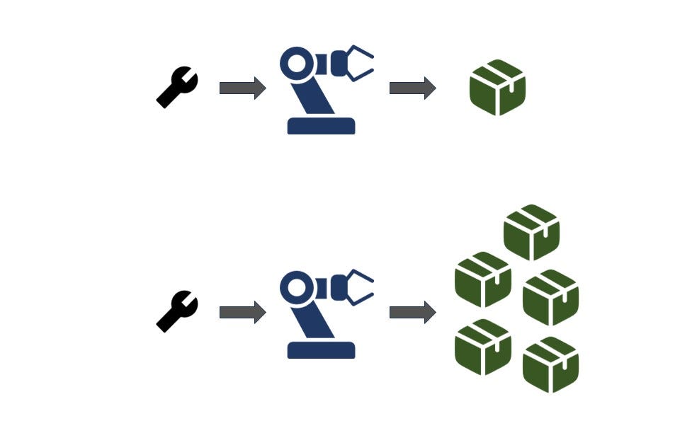
The M term — usually denoted the “big M” — should be a natural upper bound for x. It is important to define it using the smallest possible value such that the constraint is nonbinding if y equals 1. Avoiding too large values can improve linear relaxation, which has a positive effect on solver performance, besides avoiding numerical errors.

For scenarios involving multiple integer batches with limited capacity each (e.g., supply trips to a customer) we can use a similar expression. Now consider y is an integer variable denoting the number of batches performed and Q the capacity of each. The decision variable x still represents a nonnegative real value. We can write the same equation to capture our decision rules.

Batch size constraint in mixed-integer linear programming. (Image by the author).

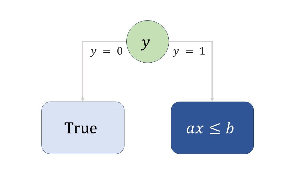
Conditional Expressions — “if-then” rules

Now imagine we want an inequality to be binding when a binary variable y is 1, else nonbinding. Once again, we can include a large value M to capture this condition.

Conditional expression in mixed-integer linear programming. (Image by the author).

In case y equals 1, the term multiplying M becomes zero and the original constraint is binding. Otherwise, M is multiplied by 1, therefore it assumes an arbitrarily large value such that the original constraint is nonbinding for any feasible value of x considering the context of the problem.

Conditional expression (inequality) that must hold when y equals one. (Image by the author).

These expressions will arise quite often in mixed-integer programming models, and some of the most common applications are detailed here.

Disjunctive rules — “if-then-else”

Disjunctive constraints are a series of connected “if-then” constraints. Additional rules ensure that either one or the other is satisfied.

Disjunctive expressions in mixed-integer linear programming. (Image by the author).

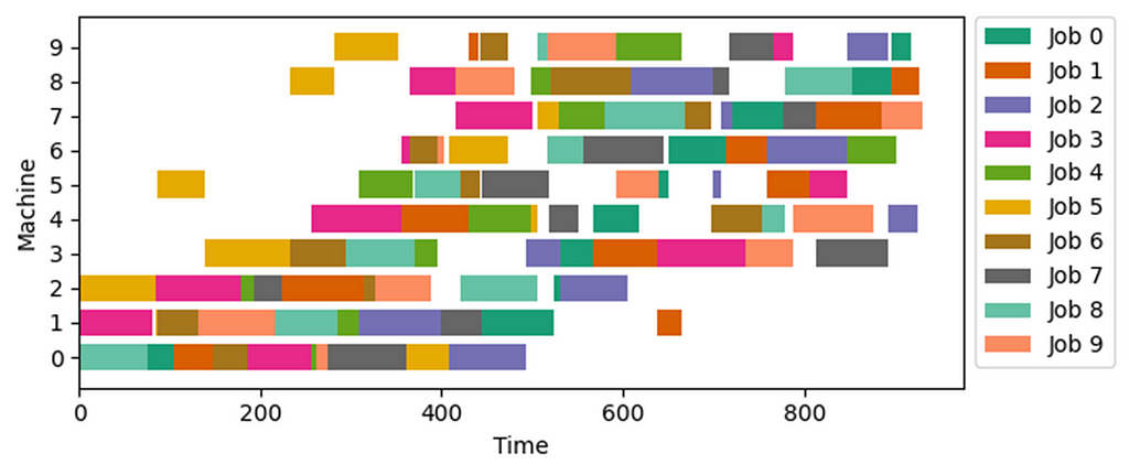
Precedence and sequences

Consider now a decision as to which operation, i or j, happens first. In some sequencing models, we can include a real-valued decision variable for the start of each operation x, another variable or a fixed parameter for its duration d, and a binary decision variable (precedence) y which is 1 if i occurs before j.

Precedence constraint in mixed-integer linear programming. (Image by the author).

These expressions will be useful in the Disjunctive Job-shop Scheduling Model and the Traveling Salesman Problem using the MTZ Formulation (Miller et al., 1960).

Gaant plot for the optimal solution of Job-shop scheduling problem with 10 jobs and 10 machines. (Image by the author).

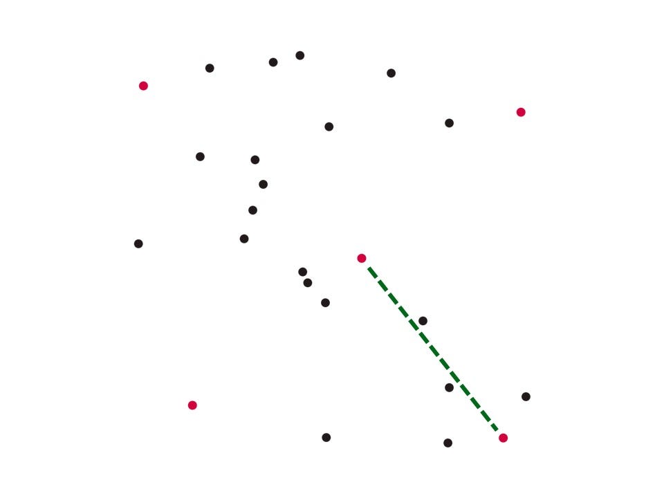
Min-max and Max-min objectives

These objectives involve the minimization of the maximum value of a set of expressions or the maximization of their minimum value. In simple terms, our goal is to keep the worst-case scenario as good as possible.

In the case of the Min-max expressions, we can create a scalar decision variable z and ensure that it is always greater than or equal to attributes d from a set of options I if the corresponding item i is selected.

Min-max expression in mixed-integer linear programming. (Image by the author).

When handling Max-min expressions, consider now z a scalar lesser than or equal to the attributes of all selected items. In both scenarios, we introduce the big M to ensure that, in case the item is not selected, the constraint becomes nonbinding. A good choice of M would be the difference between the maximum value of d (from the whole set of items) and the property of item i.

Max-min expression in mixed-integer linear programming. (Image by the author).

These expressions arise for instance in the Facility Dispersion Problem considering binary variables to indicate that a given arc or edge is active.

Maximizing the minimum distance between any five points selected in Euclidean instance of the p-dispersion problem. (Image by the author).

Discrete planning horizons

Several operations research problems include planning over a discrete horizon. In such situations, actions taken at a given moment from the timeline will affect how decisions should be performed in the future. For instance, production and inventory planning usually includes balancing between holding inventory costs, setup costs, stock coverage, and demand forecast, among other aspects. The amount produced of a given product at a given moment is usually a decision to be taken and it should affect the product availability not only when produced but also in the future when considering the possibility of stocking goods.

Inventory balance

To calculate inventory balance, let us define a discrete planning horizon T with instants t. The inventory at a given moment will be a decision variable I indexed by the elements of the set T. If we define inputs (for instance the number of items produced) and outputs (corresponding demand or items transported) of a given moment as x and d respectively, we can compute the final inventory at a given moment as the final inventory of the previous moment plus inputs minus outputs.

Graphical representation of inventory balance in a discrete planning horizon. (Image by the author).

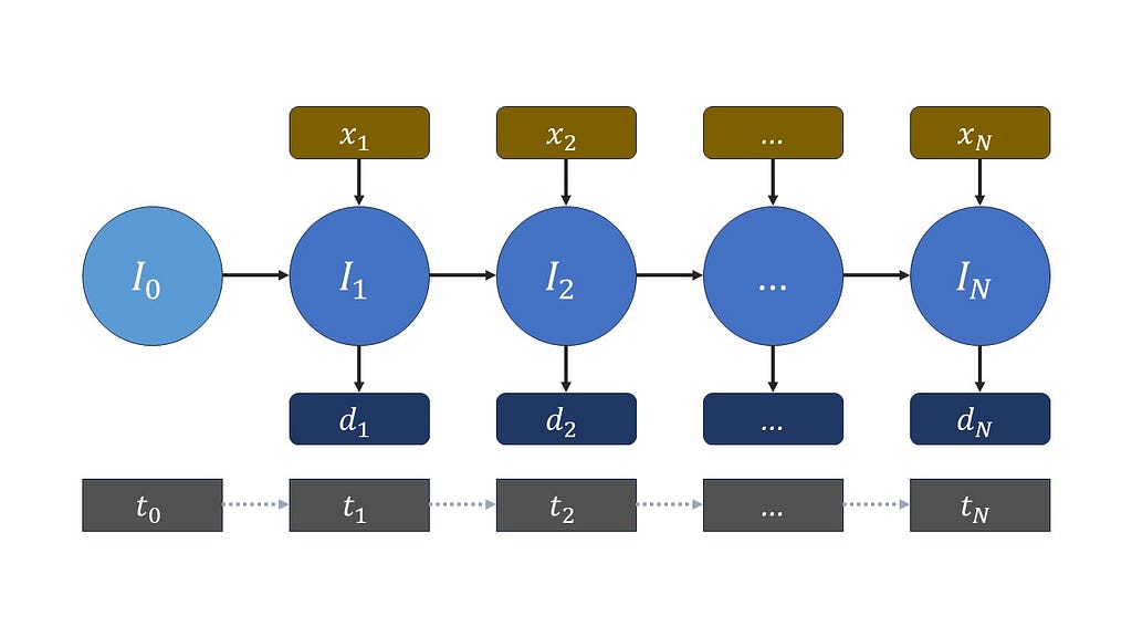
Remember the inputs and outputs might be fixed parameters of the problem or also decision variables.

We can put it in equation form as the following.

Simple inventory balance equation. (Image by the author).

A great example to illustrate this is the Dynamic Lot-Size model. However, more complex decisions might be involved in the process and new elements should be included in the inventory balance equations then. One example will be presented right next.

Inventory with backlogs

Now suppose we have deterministic demands d for each moment t, but we might decide to postpone some of them to reduce our costs (for instance setup costs or fixed charges in transportation systems). These might become backlogs in an inventory balance equation, usually with some associated cost in the objective function(s). Once again consider our inputs are represented by x, but now we are also going to include a non-negative decision variable for backlogs b, also indexed by t. The new inventory balance equation becomes the following.

Inventory balance with backlogs. (Image by the author).

Then it is up to the optimization solver to define when a demand should be postponed to reduce overall costs.

Starts and Endings

Some planning processes include scheduling activities that start at a certain moment and might last for more than one instant in the discrete planning horizon. When inserting these decisions in an optimization model, usually it is up to the model to define when the activity starts, when it ends, and possibly its corresponding duration. Therefore, we must include some binary decision variables to represent these decisions.

To a better understanding of the modeling expressions, let us visually represent an activity that starts at a given moment, is active during some instants of the planning horizon, and then ends.

Activity scheduled in a discrete planning horizon. (Image by the author).

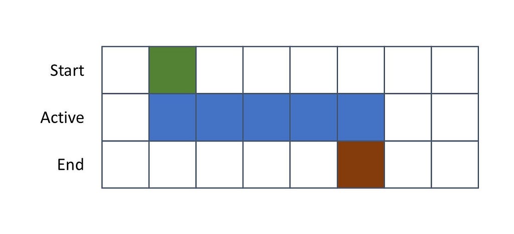
Notice that an activity starts in a moment in which it is active but it must be inactive in the previous instant. Conversely, at its ending, there’s no rule regarding the previous instant but it must be inactive in the following one.

To write that into mathematical expressions, let us use three groups of decision variables — all of them indexed by the elements of the planning horizon T. The variable x will be used to denote a moment in which the activity is active, y will denote its start, and z denote its ending.

To obtain a tight linear relaxation and help the solver during Branch & Bound, three groups of constraints will be created to establish the relationship between x and y, and the same between x and z.

To identify starts:

Set of constraints to identify the starts of an activity in a discrete planning horizon. (Image by the author).

And to identify endings:

Set of constraints to identify the endings of an activity in a discrete planning horizon. (Image by the author).

Additional implication constraints might be included in the first and last instants to ensure the desired relationships between x, y, and z in these moments.

Linearization techniques

Some problems include nonlinear expressions that cannot be incorporated directly into a MILP model. Fortunately, there are strategies involving the use of binary variables that allow us to linearize some nonlinear expressions. Two usual applications will be presented right next.

Product of real-valued and binary variables

Now, suppose we have a continuous decision variable x bounded between feasible limits L and U. Also suppose a binary decision variable y and a support decision variable z which should compute the product between x and y. When y is 1, z should assume the value of x, otherwise 0.

If y is 1, z must be greater than or equal to x (and its natural lower limit) and also lesser than or equal to x (and its natural upper limit). The only way to satisfy these inequalities is, therefore, if z is equal to x.

Now if y is 0, the last two inequalities ensure that z equals 0, while the first two inequalities ensure that any value of x between its natural bounds is feasible.

Therefore, using these inequalities, one can linearize the product between a binary and a real-valued decision variable.

Piecewise linear approximations

Now suppose we want to compute the value of a function defined in piecewise linear segments. It can be an approximation for a general nonlinear expression or simply a strategy to compute segmented linear expressions such as in contracts with distinct levels of unitary costs varying according to the volume of transactions. The idea is illustrated below by the approximation of the sigmoid function by 5 linear segments.

Sigmoid function and its corresponding piecewise linear approximation using 5 intervals. (Image by the author).

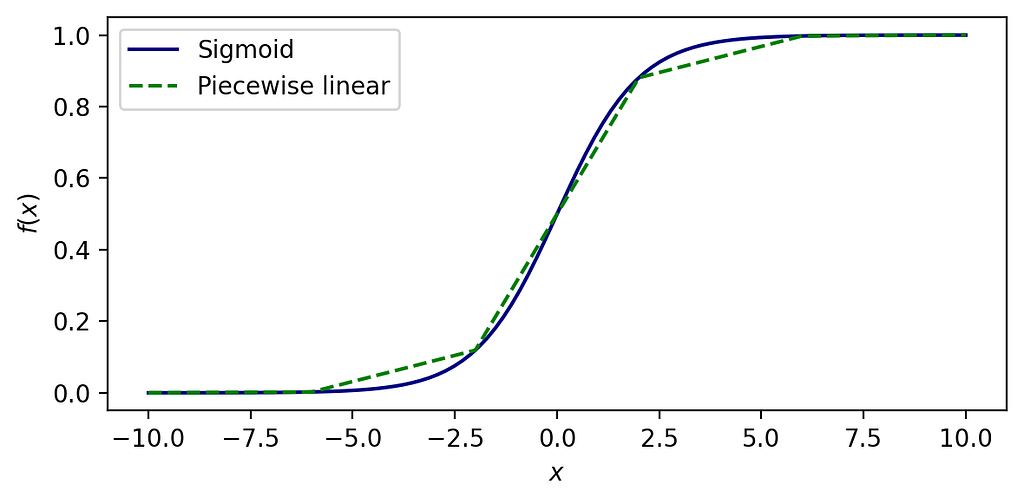
Consider a generic function f(x) defined in a given domain of a real-valued variable x between l and u. Now consider this function is discretized over N segments of arbitrary size. Each segment of index i lies between interpolation points x of indexes i and i+1, such that there are N+1 interpolation points. We now include parameters to define the linear equation of each segment:
- aᵢ: the slope of the ith linear segment
- bᵢ: the intercept of the ith linear segment
Our goal is that the decision variable y assumes the value of f(x). To do so, we also include auxiliary decision variables index by i within {1, 2, …, N}:
- zᵢ: a binary decision variable that is an indicator that x lies within the ith linear segment (closed interval).
- sᵢ: a real-valued decision variable that assumes the value of x in case it lies within the ith linear segment (closed interval).
The variable x should lie within one of the segments created, therefore a constraint must ensure that exactly one z variable is active.

Constraint ensures that one segment is active in a piecewise linear function. (Image by the author).

Now we must ensure that sᵢ equals x when zᵢ equals 1, and also compute y based on the values of sᵢ and the corresponding parameters of each segment.

Piecewise linear function constraints. (Image by the author).

Thus, using these expressions one can compute the value of a generic piecewise linear function f(x) to a real-valued decision variable y in a way that a mixed-integer linear programming solver can interpret.

Further reading

The algorithm at the core of most MILP solvers is called Branch & Bound. It efficiently explores a rooted search tree of discrete decisions without enumerating all possibilities. You might find a comprehensive introduction to this topic in my previous article.

A Gentle Introduction to Branch & Bound

Some models might resort to other techniques, such as Delayed Column Generation, which aims to solve models with a number of decision variables too large to be explicitly enumerated from the start. An introduction on this topic with a coding example can be found in a previous article too.

Column Generation in Linear Programming and the Cutting Stock Problem

Now referring to traditional books on the subject, the interested reader might refer to Numerical Optimization (Nocedal & Wright, 2006) and Linear and Nonlinear Programming (Luenberger & Ye, 2008) for a deeper understanding of optimization algorithms over continuous domain — which are often components of submodels solved in integer programming. The book Integer Programming (Wolsey, 2020) is often referred to as “the bible” of its corresponding subject. It is a great reference to understand better how exact algorithms on discrete search spaces are designed going deeper into Branch & Bound, cutting planes, and much more. The book Operations research: applications and algorithms (Winston & Goldberg, 2004) is a great alternative for those eager to see more applied examples besides a great overview of theoretical aspects.

Conclusions

Mixed-Integer Linear Programming (MILP) is a relevant area in numerical optimization with relevant applications, especially in management sciences and operations research. This article covered key expressions of MILP including Logical statements, Setup costs, Conditional expressions, Discrete planning horizons, and Linearization techniques. By combining these elements, the reader should be able to formulate real-world problems as optimization models that can be tackled by MILP solvers.

References

Luenberger, D. G. & Ye, Y., 2008. Linear and Nonlinear Programming. 3rd ed. Stanford: Springer.

Nocedal, J. & Wright, S. J., 2006. Numerical Optimization. 2nd ed. New York: Springer New York.

Winston, W. L. & Goldberg, J. B., 2004. Operations research: applications and algorithms. 4th ed. Belmont, CA: Thomson Brooks/Cole Belmont.

Wolsey, L. A., 2020. Integer Programming. 2nd ed. John Wiley & Sons.

A Comprehensive Guide to Modeling Techniques in Mixed-Integer Linear Programming was originally published in Towards Data Science on Medium, where people are continuing the conversation by highlighting and responding to this story.
Originally appeared here:
A Comprehensive Guide to Modeling Techniques in Mixed-Integer Linear Programming

Go Here to Read this Fast! A Comprehensive Guide to Modeling Techniques in Mixed-Integer Linear Programming
March 11, 2024
Optimisation: Unpacking Queueing Theory in its Simplest Terms

Khin Yadanar Lin

Have you ever found yourself waiting in line at a supermarket, a restaurant, or a bank, wishing your turn would come just a bit faster?

Continue reading on Towards Data Science »

Originally appeared here:
Optimisation: Unpacking Queueing Theory in its Simplest Terms

Go Here to Read this Fast! Optimisation: Unpacking Queueing Theory in its Simplest Terms

March 11, 2024
Making Causal Discovery work in real-world business settings
Ryan O’Sullivan
Causal AI, exploring the integration of causal reasoning into machine learning

What is this series of articles about?

Welcome to my series on Causal AI, where we will explore the integration of causal reasoning into machine learning models. Expect to explore a number of practical applications across different business contexts.

In the first article we explored using Causal Graphs to answer causal questions. This time round we will delve into making Causal Discovery work in real-world business settings.

If you missed the first article on Causal Graphs, check it out here:

Using Causal Graphs to answer causal questions

Introduction

This article aims to help you navigate the world of causal discovery.

It is aimed at anyone who wants to understand more about:
- What causal discovery is, including what assumptions it makes.
- A deep dive into conditional independence tests, the building blocks of causal discovery.
- An overview of the PC algorithm, a popular causal discovery algorithm.
- A worked case study in Python illustrating how to apply the PC algorithm.
- Guidance on making causal discovery work in real-world business settings.
The full notebook can be found here:

causal_ai/notebooks/making causal discovery work in real world business settings.ipynb at main · raz1470/causal_ai

What is Causal Discovery?

In my last article, I covered how causal graphs could be used to answer causal questions.

Often referred to as a DAG (directed acyclic graph), a causal graph contains nodes and edges — Edges link nodes that causally related.

There are two ways to determine a causal graph:
- Expert domain knowledge
- Causal discovery algorithms
We don’t always have the expert domain knowledge to determine a causal graph. In this notebook we will explore how to take observational data and determine the causal graph using causal discovery algorithms.

Algorithms

Causal discovery is a heavily researched area in academia with four groups of methods proposed:

It isn’t clear from currently available research which method is best. One of the challenges in answering this question is the lack of realistic ground truth benchmark datasets.

Image by author

In this blog we are going to focus on understanding the PC algorithm, a constraint-based method that uses conditional independence tests.

Assumptions

Before we introduce the PC algorithm, let’s cover the key assumptions made by causal discovery algorithms:
1. Causal Markov Condition: Each variable is conditionally independent of its non-descendants, given its direct causes. This tells us that if we know the causes of a variable, we don’t gain any additional power by knowing the variables that are not directly influenced by those causes. This fundamental assumption simplifies the modelling of causal relationships enabling us to make causal inferences.
2. Causal Faithfulness: If statistical independence holds in the data, then there is no direct causal relationships between the corresponding variables. Testing this assumption is challenging and violations may indicate model misspecification or missing variables.
3. Causal Sufficiency: Are the variables included sufficient to make causal claims about the variables of interest? In other words, we need all confounders of the variables included to be observed. Testing this assumption involves sensitivity analysis which assesses the impact of potentially unobserved confounders.
4. Acyclicity: No cycles in the graph.
In practice, while these assumptions are necessary for causal discovery, they are often treated as assumptions rather than directly tested.

Even with making these assumptions, we can end up with a Markov equivalence class. We have a Markov equivalence class when we have multiple causal graphs each as likely as each other.

Conditional Independence tests

Conditional independence tests are the building blocks of causal discovery and are used by the PC algorithm (which we will cover shortly).

Let’s start by understanding independence. Independence between two variables implies that knowing the value of one variable provides no information about the value of the other. In this case, it is fairly safe to assume that neither directly causes the other. However, if two variables aren’t independent, it would be wrong to blindly assume causation.

Conditional independence tests can be used to determine whether two variables are independent of each other given the presence of one or more other variables. If two variables are conditionally independent, we can then infer that they are not causally related.

The Fisher’s exact test can be used to determine if there is a significant association between two variables whilst controlling for the effects of one or more additional variables (use the additional variables to split the data into subsets, the test can then be applied to each subset of data). The null hypothesis assumes that there is no association between the two variables of interest. A p-value can then be calculated and if it is below 0.05 the null hypothesis will be rejected suggesting that there is significant association between the variables.

Identifying spurious correlations

We can use an example of a spurious correlation to illustrate how to use conditional independence tests.

Two variables have a spurious correlation when they have a common cause e.g. High temperatures increasing the number of ice cream sales and shark attacks.
```
np.random.seed(999)

# Create dataset with spurious correlation
temperature = np.random.normal(loc=0, scale=1, size=1000)
ice_cream_sales = 2.5 * temperature + np.random.normal(loc=0, scale=1, size=1000)
shark_attacks = 0.5 * temperature + np.random.normal(loc=0, scale=1, size=1000)
df_spurious = pd.DataFrame(data=dict(temperature=temperature, ice_cream_sales=ice_cream_sales, shark_attacks=shark_attacks))

# Pairplot
sns.pairplot(df_spurious, corner=True)
```
Image by author
```
# Create node lookup variables
node_lookup = {0: 'Temperature',
               1: 'Ice cream sales',
               2: 'Shark attacks'                                                                          
 }

total_nodes = len(node_lookup)

# Create adjacency matrix - this is the base for our graph
graph_actual = np.zeros((total_nodes, total_nodes))

# Create graph using expert domain knowledge
graph_actual[0, 1] = 1.0 # Temperature -> Ice cream sales
graph_actual[0, 2] = 1.0 # Temperature -> Shark attacks
     
plot_graph(input_graph=graph_actual, node_lookup=node_lookup)
```
Image by author

The following conditional independence tests can be used to determine the causal graph:
```
# Run first conditional independence test
test_id_1 = round(gcm.independence_test(ice_cream_sales, shark_attacks, conditioned_on=temperature), 2)

# Run second conditional independence test
test_id_2 = round(gcm.independence_test(ice_cream_sales, temperature, conditioned_on=shark_attacks), 2)

# Run third conditional independence test
test_id_3 = round(gcm.independence_test(shark_attacks, temperature, conditioned_on=ice_cream_sales), 2)
```
Image by author

Although we don’t know the direction of the relationships, we can correctly infer that temperature is causally related to both ice cream sales and shark attacks.

PC algorithm

The PC algorithm (named after its inventors Peter and Clark) is a constraint-based causal discovery algorithm that uses conditional independence tests.

It can be summarised into 2 main steps:
1. It starts with a fully connected graph and then uses conditional independence tests to remove edges and identify the undirected causal graph (nodes linked but with no direction).
2. It then (partially) directs the edges using various orientation tricks.
We can use the previous spurious correlation example to illustrate the first step:
- Start with a fully connected graph
- Test ID 1: Accept the null hypothesis and delete edge, no causal link between ice cream sales and shark attacks
- Test ID 2: Reject the null hypothesis and keep the edge, causal link between ice cream sales and temperature
- Test ID 3: Reject the null hypothesis and keep the edge, causal link between shark attacks and ice cream sales
Evaluating results

One of the key challenges in causal discovery is evaluating the results. If we knew the causal graph, we wouldn’t need to apply a causal discovery algorithm! However, we can create synthetic datasets to evaluate how well causal discovery algorithms perform.

There are several metrics we can use to evaluate causal discovery algorithms:

Image by author
- True positives: Identify causal link correctly
- False positives: Identify causal link incorrectly
- True negatives: Correctly identify no causal link
- False negatives: Incorrectly identify no causal link
- Reversed edges: Identify causal link correctly but in the wrong direction
We want a high number of True positives, but this should not be at the expense of a high number of False positives (as when we come to build an SCM, wrong causal links can be very damaging). Therefore GScore seems to capture this well whilst giving an interpretable ratio between 0 and 1.

Call Centre case study

We will revisit the call centre case study from my previous article. First of all, we determine the causal graph (to be used as ground truth) and then use our knowledge of the data-generating process to create some samples.

The ground truth causal graph and generated samples will enable us to evaluate the PC algorithm.
```
# Create node lookup for channels
node_lookup = {0: 'Demand',
               1: 'Call waiting time',
               2: 'Call abandoned', 
               3: 'Reported problems',                   
               4: 'Discount sent',
               5: 'Churn'                                                                             
 }

total_nodes = len(node_lookup)

# Create adjacency matrix - this is the base for our graph
graph_actual = np.zeros((total_nodes, total_nodes))

# Create graph using expert domain knowledge
graph_actual[0, 1] = 1.0 # Demand -> Call waiting time
graph_actual[0, 2] = 1.0 # Demand -> Call abandoned
graph_actual[0, 3] = 1.0 # Demand -> Reported problems
graph_actual[1, 2] = 1.0 # Call waiting time -> Call abandoned
graph_actual[1, 5] = 1.0 # Call waiting time -> Churn
graph_actual[2, 3] = 1.0 # Call abandoned -> Reported problems
graph_actual[2, 5] = 1.0 # Call abandoned -> Churn
graph_actual[3, 4] = 1.0 # Reported problems -> Discount sent
graph_actual[3, 5] = 1.0 # Reported problems -> Churn
graph_actual[4, 5] = 1.0 # Discount sent -> Churn

plot_graph(input_graph=graph_actual, node_lookup=node_lookup)
```
Image by author
```
def data_generator(max_call_waiting, inbound_calls, call_reduction):
    '''
     A data generating function that has the flexibility to reduce the value of node 0 (Call waiting time) - this enables us to calculate ground truth counterfactuals

    Args:
        max_call_waiting (int): Maximum call waiting time in seconds
        inbound_calls (int): Total number of inbound calls (observations in data)
        call_reduction (float): Reduction to apply to call waiting time

    Returns:
        DataFrame: Generated data
    '''
    
    df = pd.DataFrame(columns=node_lookup.values())

    df[node_lookup[0]] = np.random.randint(low=10, high=max_call_waiting, size=(inbound_calls)) # Demand
    df[node_lookup[1]] = (df[node_lookup[0]] * 0.5) * (call_reduction) + np.random.normal(loc=0, scale=40, size=inbound_calls) # Call waiting time
    df[node_lookup[2]] = (df[node_lookup[1]] * 0.5) + (df[node_lookup[0]] * 0.2) + np.random.normal(loc=0, scale=30, size=inbound_calls) # Call abandoned
    df[node_lookup[3]] = (df[node_lookup[2]] * 0.6) + (df[node_lookup[0]] * 0.3) + np.random.normal(loc=0, scale=20, size=inbound_calls) # Reported problems
    df[node_lookup[4]] = (df[node_lookup[3]] * 0.7) + np.random.normal(loc=0, scale=10, size=inbound_calls) # Discount sent
    df[node_lookup[5]] = (0.10 * df[node_lookup[1]] ) + (0.30 * df[node_lookup[2]]) + (0.15 * df[node_lookup[3]]) + (-0.20 * df[node_lookup[4]]) # Churn

    return df

# Generate data
np.random.seed(999)
df = data_generator(max_call_waiting=600, inbound_calls=10000, call_reduction=1.00)

# Pairplot
sns.pairplot(df, corner=True)
```
Image by author

Applying the PC algorithm

The Python package gCastle has several causal discovery algorithms implemented, including the PC algorithm:

trustworthyAI/gcastle at master · huawei-noah/trustworthyAI

When we feed the algorithm our samples we receive back the learned causal graph (in the form of an adjacency matrix).
```
# Apply PC method to learn graph
pc = PC(variant='stable')
pc.learn(df)
graph_pred = pc.causal_matrix

graph_pred
```
Image by author

gCastle also has several evaluation metrics available, including gScore. The GScore of our learned graph is 0! Why has it done so poorly?
```
# GScore
metrics = MetricsDAG(
    B_est=graph_pred, 
    B_true=graph_actual)
metrics.metrics['gscore']
```
Image by author

On closer inspection of the learned graph, we can see that it correctly identified the undirected graph and then struggled to orient the edges.
```
plot_graph(input_graph=graph_pred, node_lookup=node_lookup)
```
Image by author

Evaluating the undirected graph

To build on the learning from applying the PC algorithm, we can use gCastle to extract the undirected causal graph that was learned.
```
# Apply PC method to learn skeleton
skeleton_pred, sep_set = find_skeleton(df.to_numpy(), 0.05, 'fisherz')

skeleton_pred
```
Image by author

If we transform our ground truth graph into an undirected adjacency matrix, we can then use it to calculate the Gscore of the undirected graph.
```
# Transform the ground truth graph into an undirected adjacency matrix
skeleton_actual = graph_actual + graph_actual.T
skeleton_actual = np.where(skeleton_actual > 0, 1, 0)
```
Using the learned undirected causal graph we get a GScore of 1.00.
```
# GScore
metrics = MetricsDAG(
    B_est=skeleton_pred, 
    B_true=skeleton_actual)
metrics.metrics['gscore']
```
Image by author

We have accurately learned an undirected graph — could we use expert domain knowledge to direct the edges? The answer to this will vary across different use cases, but it is a reasonable strategy.
```
plot_graph(input_graph=skeleton_pred, node_lookup=node_lookup)
```
Image by author

Making Causal Discovery work in real-world business settings

We need to start seeing causal discovery as an essential EDA step in any causal inference project:
- However, we also need to be transparent about its limitations.
- Causal discovery is a tool that needs complementing with expert domain knowledge.
Be pragmatic with the assumptions:
- Can we ever expect to observe all confounders? Probably not. However, with the correct domain knowledge and extensive data gathering, it is feasible that we could observe all the key confounders.
Pick an algorithm where we can apply constraints to incorporate expert domain knowledge — gCastle allows us to apply constraints to the PC algorithm:
- Initially work on identifying the undirected causal graph and then share this output with domain experts and use them to help orient the graph.
Be cautious when using proxy variables and consider enforcing constraints on relationships we strongly believe exist:
- For example, if include Google trends data as a proxy for product demand, we may need to enforce constraints in terms of this driving sales.
Future work
- What if we have non-linear relationships? Can the PC algorithm handle this?
- What happens if we have unobserved confounders? Can the FCI algorithm deal with this situation effectively?
- How do constraint-based, score-based, functional-based and gradient-based methods compare?
Follow me if you want to continue this journey into Causal AI — In the next article we will understand how Double Machine Learning can help de-bias treatment effects.

Making Causal Discovery work in real-world business settings was originally published in Towards Data Science on Medium, where people are continuing the conversation by highlighting and responding to this story.
Originally appeared here:
Making Causal Discovery work in real-world business settings

Go Here to Read this Fast! Making Causal Discovery work in real-world business settings
March 11, 2024
How To Create A Successful Data Presentation

Rashi Desai

Present your data like a pro in five easy steps…

Continue reading on Towards Data Science »

Originally appeared here:
How To Create A Successful Data Presentation

Go Here to Read this Fast! How To Create A Successful Data Presentation

March 11, 2024
Supercharged pandas: Tracing dependencies with a novel approach
Ji Wei Liew
Supercharged Pandas: Tracing Dependencies with a Novel Approach

An object-oriented approach to manage multiple files and dataframes, and tracing dependencies.

Photo by Sibel Yıldırım on Unsplash

How will this benefit you:

This article describes an object-oriented approach for data analysis. It outlines 2 novel approaches: (a) reduce repetitive file reads by assigning dataframes to the attributes of the Reports object, and (b) trace dependent methods recursively to construct attributes. These approaches have allowed me to be highly productive in what I do and I hope that you will reap similar benefits.

Who should read this:
- You have to analyze the same data set over a long period of time.
- You need to build reports by combining data from different sources and prepare statistics.
- You have co-workers who tend to ask you, “How did you arrive at this data?” and you cannot recall the N steps in Excel that you took to prepare the report.
- You have been using pandas for a while and you suspect that there is a more efficient way of doing things.
What’s in this article?
- Monolithic script: how it begins
- Reusable functions: how it progresses
- Objects, methods and attributes: how it evolves
- Tracing upstream dependencies: a novel approach
Preamble

It is rather difficult to explain what I am trying to do, so please bear with me if the first half of this article doesn’t make sense. I promise that towards the end, it will be all worth it.

Monolithic script: how it begins

Suppose you have 3 csv files: file1.csv, file2.csv, file3.csv. You write some code to read each one of them, and then merge them in a particular order.
```
df1 = pd.read_csv('file1.csv')
df2 = pd.read_csv('file2.csv')
df3 = pd.read_csv('file3.csv')

df1_2 = pd.merge(df1, df2, on='a', how='left')
df1_2_3 = pd.merge(df1_2, df3, on='b', how='inner')
```
This works perfect, and you get on with life. Next, your boss gives you file4.csv which is supposed to be merged with file1.csv to build a separate report. No issues, you know the drill, you update the code:
```
df1 = pd.read_csv('file1.csv')
df2 = pd.read_csv('file2.csv')
df3 = pd.read_csv('file3.csv')
df4 = pd.read_csv('file4.csv')

df1_2 = pd.merge(df1, df2, on='a', how='left')
df1_2_3 = pd.merge(df1_2, df3, on='b', how='inner')
df1_4 = pd.merge(df1, df4, on='a', how='left')
```
The code runs smoothly and you get the desired output. Boss pats you on the back and jokingly says, “That’s quick, can you be even faster?”

You look up at your boss, but all you can see is a train of expletives flashing across your eyes. You fight the visceral urge to pick one to be processed by your biological audio output device. You triumphed in doing so and summoned all the hypocritical chakra to fake a smile and respond cheerfully, “Sure, let me give it a shot.”

As the train of expletives fades into the horizon and as you exhaust all your chakra, you noticed a glimmer of hope: there is no need to read file2.csv and file3.csv if you are only interested in df1_4. It dawn upon you that this flagrant expenditure of precious time and computing power, contradicts with your commitment towards sustainability and you begin to contemplate how to make the code more efficient by reading only what is necessary.

Reusable functions: how it progresses

You recall the programming classes that you took N years ago and proceeded to write some functions:
```
files = {1: 'file1.csv', 2: 'file2.csv', 3:'file3.csv', 4:'file4.csv'}

def get_df(x):
    return pd.read_csv(files[x])

def get_df1_2():
    df1 = get_df(1)
    df2 = get_df(2)
    return pd.merge(df1, df2, on='a', how='left')  

def get_df1_2_3():
    df1_2 = get_df1_2()
    df3 = get_df(3)
    return pd.merge(df1_2, df3, on='b', how='inner')

def get_df1_4():
    df1 = get_df(1)
    df4 = get_df(4)
    return pd.merge(df1, df4, on='a', how='left')
```
You are pleased with yourself. Although the number of lines of code has more than doubled, you take comfort in the fact that it will be more manageable in the long run. Also, you justify this approach because you can get specific output dataframes and each one of them will only read the required tables and nothing else. You feel a chill down your spine, as an inner voice challenges your conscious thoughts. “Are you sure?” he barked in a commanding tone, reminiscent of a drill sergeant. Silence hung densely in the air, and all you can hear is the spinning of the imaginary cogs in your mind… Suddenly, your eyes lit up and noticed that if you need df1_2 and df1_4, then file1.csv will be read twice! Roar!

Objects, methods and attributes: how it evolves

Once again, you recall the programming lessons in college and remembered that you can resolve this by creating a Reports object. After a dataframe has been read, it can be set as an attribute of the Reports object so that it can be accessed later.
```
files = {1: 'file1.csv', 2: 'file2.csv', 3:'file3.csv', 4:'file4.csv'}

class Reports:
    
    def __init__(self):
        self.df1 = pd.read_csv(files[1])

    def get_df1_2(self):
        self.df2 = pd.read_csv(files[2])
        self.df1_2 = pd.merge(self.df1, self.df2, on='a', how='left')
        return self.df1_2

    def get_df1_4(self):
        self.df4 = pd.read_csv(files[4])
        self.df1_4 = pd.merge(self.df1, self.df4, on='a', how='left')

    def get_df1_2_3(self):
        self.get_df1_2()  
        self.df3 = pd.read_csv(files[3])
        self.df1_2_3 = pd.merge(self.df1_2, self.df3, on='b', how='inner')
```
Voila! You have solved the problem of reading the same file several times. But there is yet another problem: get_df1_2_3 can get very complicated if it has to go through many steps, e.g. filtering, selecting, boolean-masking, removal of duplicates, etc.

Tracing upstream dependencies: a novel approach

You take a deep breath and wonder… is there a way for the code to figure out that if self.df1_2 has not been set, then it should call self.get_df1_2()? More generally, when an attribute being accessed is not present, can we identify which method is responsible for setting it, and then call the method? If this can be achieved, then one can use x=Reports(); x.df1_2_3 to get to the required dataframe in one command.

Isn’t that worth fighting for? Isn’t that worth dying? — Morpheus, The Matrix Reloaded, 2003

Like a mad scientist at work, you begin hammering away at your keyboard, occasionally looking up to make imaginary drawings of programming abstractions and connecting them with your fingers. From your peripheral, you notice the look of bewilderment — or perhaps disgust, but you couldn’t tell — from a co-worker you never knew. You channel all your focus to enter flow state, oblivious to what is happening around you. The building could have caught fire, but you wouldn’t know as long as your trusty Notepad++ continues to display every key you enter.
```
files = {'df1': 'file1.csv', 'df2': 'file2.csv',
         'df3': 'file3.csv', 'df4': 'file4.csv'}

class Reports:
    
    def __init__(self):
        self._build_shortcuts()
    
    def _read(self, k):
        setattr(self, k, pd.read_csv(files[k]))  

    def _build_shortcuts(self):
        # Dict: Method -> list of attributes
        dict0 = {'get_df1_2': ['df1_2'],
                 'get_df1_4': ['df1_4'],
                 'get_df1_2_3': ['df1_2_3']}

        # Dict: Attribute -> method which creates the attribute
        dict1 = {v:k for k, values in dict0.items() for v in values}
        self._shortcuts = dict1

    def __getattr__(self, attr):
        if not attr in self.__dict__: # if the attr has not been created...
            if attr in self._shortcuts: 
                func = self._shortcuts[attr] 
                # `func` is the method responsible for creating attr
                self.__getattribute__(func)()
                return self.__getattribute__(attr)
            elif attr in files:
                self._read(attr)
                return self.__getattribute__(attr)
            else:
                raise AttributeError
        else:
            return self.__getattribute__(attr)
  
    def get_df1_2(self):
        self.df1_2 = pd.merge(self.df1, self.df2, on='a', how='left')
        return self.df1_2

    def get_df1_4(self):
        self.df1_4 = pd.merge(self.df1, self.df4, on='a', how='left')
        return self.df1_4
    
    def get_df1_2_3(self):
        self.df1_2_3 = pd.merge(self.df1_2, self.df3, on='b', how='inner')
        return self.df1_2_3
```
You take a moment to admire your creation, its elegance and simplicity. For a split second, you dream about how this will benefit coders and data analysts. As you ride the hot-air balloon of euphoria, the inner voice descends upon you like shackles on a prisoner. “Stay grounded,” he said, “as you may not be the first to come up with such an idea.” You buckle down and begin documenting your work, consciously aware that you may not understand what you have written a few days later.

__init__() does not read files. It merely calls build_shortcuts().
- _build_shortcuts() & __getattr__ work hand-in-hand to simplify the code in subsequent methods.
- _build_shortcuts() takes a dictionary with methods as keys and list of attributes as values, then inverts it to form a dictionary with attributes as keys and methods which sets the attributes as values.
- __getattr__ does quite a bit of magic. When one calls self.<attr>, if attr is not present in self.__dict__ but is in self._shortcuts, then it identifies the method that is responsible for creating self.<attr> and calls the method. Whenever you create a new method, if it sets a new attribute, then all you have to do is to update dict0 in self._build_shortcuts(). If it is in the keys of the files dictionary, then it reads the corresponding file and sets the key as the attribute of the Reports object.
- Without explicitly writing a loop or recursion, __getattr__ and self._shortcuts work together to trace the upstream dependencies!
For now, this is a superior approach for the following reasons:
- Files are read only when absolutely required, minimal time wasted.
- When files are read, they are read only once, and data written to the attribute.
- When calling an attribute, if it is not created, it will find the method responsible for setting the attribute, and then set it.
Additional benefit

Besides being able to access the desired dataframes in one command, you can also add other attributes[1] to the values of dict0 in _build_shortcuts().

For example, you may be interested in the list of unique values of column a in df1_2. Simply add it to the list, and you can use x = Reports(); x.unique_values_in_a.
```
    ...
    
    def _build_shortcuts(self):

        # Added 'unique_items_in_a' to the first list.
        dict0 = {'get_df1_2': ['df1_2', 'unique_values_in_a'],
                 'get_df1_4': ['df1_4'],
                 'get_df1_2_3': ['df1_2_3']}


        dict1 = {v:k for k, values in dict0.items() for v in values}
        self._shortcuts = dict1
    ...

    def get_df1_2(self):
        self.df1_2 = pd.merge(self.df1, self.df2, on='a', how='left')
        # Added the list of unique values of column 'a'
        self.unique_values_in_a = self.df1_2['a'].unique().tolist()
        return self.df1_2
```
Conclusion

What does it mean for you?

I highly encourage you to try this approach the next time you are required to analyze data which involving multiple dataframes.
- For python novices, you can just copy-and-paste the Reports class, __init__, __getattr__ and _build_shortcuts method. Obviously, you will need to write your own methods and updatedict0 in _build_shortcuts.
- For python experts, I would love to hear your view on my approach and if you are doing something similar, or better.
Disclaimer

This narrative is merely for illustrative purposes and does not in any way shape or form represent my or my firm’s views or reflect in any way experiences in my firm or with my clients.

This is the first time that I’ve used such a writing style, if you like it, do show your appreciation by clapping, following and subscribing. Thank you!

[1] Many thanks to Tongwei for proofreading and suggesting this.

Supercharged pandas: Tracing dependencies with a novel approach was originally published in Towards Data Science on Medium, where people are continuing the conversation by highlighting and responding to this story.
Originally appeared here:
Supercharged pandas: Tracing dependencies with a novel approach

Go Here to Read this Fast! Supercharged pandas: Tracing dependencies with a novel approach
March 11, 2024
Craft A Customized Word Cloud Trivia Game with Python

Lee Vaughan

Tailor game night to your interests!

Continue reading on Towards Data Science »

Originally appeared here:
Craft A Customized Word Cloud Trivia Game with Python

Go Here to Read this Fast! Craft A Customized Word Cloud Trivia Game with Python

March 10, 2024
An Overview of the LoRA Family
Dorian Drost
LoRA, DoRA, AdaLoRA, Delta-LoRA, and more variants of low-rank adaptation.

LoRA comes in different shapes and varieties. Photo by Lucas George Wendt on Unsplash.

Low-Rank Adaptation (LoRA) can be considered a major breakthrough towards the ability to train large language models for specific tasks efficiently. It is widely used today in many applications and has inspired research on how to improve upon its main ideas to achieve better performance or train models even faster.

In this article, I want to give an overview of some variants of LoRA, that promise to improve LoRAs capabilities in different ways. I will first explain the basic concept of LoRA itself, before presenting LoRA+, VeRA, LoRA-FA, LoRA-drop, AdaLoRA, DoRA, and Delta-LoRA. I will introduce the basic concepts and main ideas each, and show, how these approaches deviate from the original LoRA. I will spare technical details, unless they are important for the basic concepts, and will also not discuss evaluations in detail. For readers interested, I linked the original papers at the end.

Lora

The main idea of LoRA is to add two smaller tunable matrices A and B next to the pre-trained weight matrix W, without changing the parameters of W. Image from [1].

Low-Rank Adaption (LoRA) [1] is a technique, that is widely used today to train large language models (LLMs). Large language models come with the capability to predict tokens of natural language given a natural language input. This is an astonishing capability, but for solving many problems this is not enough. Most of the time, you want to train an LLM on a given downstream task, such as classifying sentences or generating answers to given questions. The most straightforward way of doing that is fine-tuning, where you train some of the layers of the LLM with data of the desired task. That means training very big models with millions to billions of parameters though.

LoRA gives an alternative way of training that is much faster and easier to conduct due to a drastically reduced number of parameters. Next to the parameter weights of an already pre-trained LLM layer, LoRA introduces two matrices A and B, that are called adapters and that are much smaller. If the original matrix of parameters W is of size d x d, the matrices A and B are of size d x r and r x d, where r is much smaller (typically below 100). The parameter r is called the rank. That is, if you use LoRA with a rank of r=16, these matrices are of shape 16 x d. The higher the rank, the more parameters you train. That can lead to better performance on the one hand but needs more computation time on the other.

Now that we have these new matrices A and B, what happens with them? The input fed to W is also given to B*A, and the output of B*A is added to the output of the original matrix W. That is, you train some parameters on top and add their output to the original prediction, which allows you to influence the model’s behavior. You don’t train W anymore, which is why we sometimes say that W is frozen. Importantly, the addition of A and B is not only done at the very end (which would just add a layer on top) but can be applied to layers deep inside the neural network.

That is the main idea of LoRA, and its biggest advantage is, that you have to train fewer parameters than in fine-tuning, but still get comparable performance. One more technical detail I want to mention at this place: At the beginning, the matrix A is initialized with random values of mean zero, but with some variance around that mean. The matrix B is initialized as a matrix of complete zeros. This ensures, that the LoRA matrices don’t change the output of the original W in a random fashion from the very beginning. The update of A and B on W’s output should rather be an addition to the original output, once the parameters of A and B are being tuned in the desired direction. However, we will later see that some approaches deviate from this idea for different reasons.

LoRA as just explained is used very often with today’s LLMs. However, by now there are many variants of LoRA that deviate from the original method in different ways and aim at improving speed, performance, or both. Some of these I want to present to you in the following.

LoRA+

LoRA+ introduces different learning rates for the two matrices A and B, here indicated by the parameter λ. Image from [2].

LoRA+ [2] introduces a more efficient way of training LoRA adapters by introducing different learning rates for matrices A and B. Most of the time, when training a neural network, there is just one learning rate that is applied to all weight matrices the same way. However, for the adapter matrices used in LoRA, the authors of LoRA+ can show, that it is suboptimal to have that single learning rate. The training becomes more efficient by setting the learning rate of matrix B much higher than that of matrix A.

There is a theoretical argument to justify that approach, that mainly bases on numerical caveats of a neural network’s initialization if the model becomes very wide in terms of the number of its neurons. However, the math required to prove that is quite complicated (if you are really into it, feel free to take a look at the original paper [2]). Intuitively, you may think that matrix B, which is initialized with zero, could use bigger update steps than the randomly initialized matrix A. In addition, there is empirical evidence for an improvement by that approach. By setting the learning rate of matrix B 16 times higher than that of matrix A, the authors have been able to gain a small improvement in model accuracy (around 2%), while speeding up the training time by factor two for models such as RoBERTa or Llama-7b.

VeRA

VeRA doesn’t train A and B, but initializes them to a random projection and trains additional vectors d and b instead. Image from [3].

With VeRA (Vector-based Random Matrix Adaptation) [3], the authors introduce an approach to drastically reduce the parameter size of the LoRA adapters. Instead of training the matrices A and B, which is the core idea of LoRA in the first place, they initialize these matrices with shared random weights (i.e. all the matrices A and B in all the layers have the same weights) and add two new vectors d and b. Only these vectors d and b are trained in the following.

You may wonder how this can work at all. A and B are matrices of random weights. How should they contribute anything to the model’s performance, if they are not trained at all? This approach is based on an interesting field of research on so-called random projections. There is quite some research that indicates that in a large neural network only a small fraction of the weights is used to steer the behavior and lead to the desired performance on the task the model was trained for. Due to the random initialization, some parts of the model (or sub-networks) are contributing more towards the desired model behavior from the very beginning. During the training, all parameters are trained though, as it is now known which are the important subnetworks. That makes training very costly, as most of the parameters that are updated don’t add any value to the model’s prediction.

Based on this idea, there are approaches to only train these relevant sub-networks. A similar behavior can be obtained by not training the sub-networks themselves, but by adding projection vectors after the matrix. Due to the multiplication of the matrix with the vector, this can lead to the same output as tuning some sparse parameters in the matrix would. That is exactly what the authors of VeRA propose by introducing the vectors d and b, which are trained, while the matrices A and B are frozen. Also, in contrast to the original LoRa approach, matrix B is not set to zero anymore but is initialized randomly just as matrix A.

This approach naturally leads to a number of parameters that is much smaller than the full matrices A and B. For example, if you introduce LoRA-layers of rank 16 to GPT-3, you would have 75.5M parameters. With VeRA, you only have 2.8M (a reduction of 97%). But how is the performance with such a small number of parameters? The authors of VeRA performed an evaluation with some common benchmarks such as GLUE or E2E and with models based on RoBERTa and GPT2 Medium. Their results suggest, that the VeRA model yields performance that is only marginally lower than models that are fully finetuned or that use the original LoRa technique.

LoRA-FA

LoRA-FA freezes matrix A and only trains matrix B. Image from [4].

Another approach, LoRA-FA [4], which stands for LoRA with Frozen-A, is going in a similar direction as VeRA. In LoRA-FA, the matrix A is frozen after initialization and hence serves as a random projection. Instead of adding new vectors, matrix B is trained though, after being initialized with zeros (just as in the original LoRA). This halves the number of parameters while having comparable performance to normal LoRA.

LoRa-drop

LoRA-drop uses the output of B*A to decide, which LoRA-layers are worth to be trained at all. Image from [5].

In the beginning, I explained, that you can add Lora matrices to any layer in the neural network. LoRA-drop [5] introduces an algorithm to decide which layers are worth to be enhanced by LoRA, and for which this is not worth the effort. Even if training LoRA adapters is much cheaper than finetuning the whole model, the more LoRA adapters you add, the more expensive is the training, still.

LoRA-drop consists of two steps. In the first step, you sample a subset of the data and train the LoRA adapters for a few iterations. Then you calculate the importance of each LoRA adapter as B*A*x, where A and B are the LoRA matrices, and x is the input. That is simply the output of the LoRA adapters that is added to the output of the frozen layer each. If this output is big, it changes the behavior of the frozen layer more drastically. If it is small, this indicates that the LoRA adapter has only little influence on the frozen layer and could as well be omitted.

Given that importance, you now select the LoRA layers that are most important. The are different ways of doing that. You can sum up the importance values until you reach a threshold, which is controlled by a hyperparameter, or you just take the top n LoRA layers with the highest importance for a fixed n. In any case, in the next step, you conduct the full training on the whole dataset (remember that you used a subset of data for the previous steps) but only on those layers that you just selected. The other layers are fixed to a shared set of parameters that won’t be changed anymore during training.

The algorithm of LoRA-drop hence allows to training a model with just a subset of the LoRA layers. The authors propose empirical evidence that indicates only marginal changes in accuracy, compared to training all LoRA layers, but at reduced computation time due to the smaller number of parameters that have to be trained.

AdaLoRA

AdaLoRA allows to adapt the rank of the LoRA matrices dynamically. Photo by Hasmik Ghazaryan Olson on Unsplash

There are alternative ways how to decide which LoRA parameters are more important than others. In this section, I will present AdaLoRA [6], which stands for Adaptive LoRa. What part of LoRA is adaptive here? It is the rank (i.e. the size) of the LoRA matrices. The main problem is the same as in the previous section: It may not be worth adding LoRA matrices A and B to each layer, but for some layers, the LoRA training may be more important (i.e. may lead to more change in the model’s behavior) than for others. To decide on that importance, the authors of AdaLoRA propose to consider the singular values of the LoRA matrices as indicators of their importance.

What is meant by that? First, we have to understand, that a matrix multiplication can also be seen as applying a function to a vector. When dealing with neural networks, this is quite obvious: Most of the time you use neural networks as functions, i.e. you give an input (say, a matrix of pixel values) and obtain a result (say, a classification of an image). Under the hood, this function application is powered by a sequence of matrix multiplications. Now, let’s say you want to reduce the number of parameters in such a matrix. That will change the function’s behavior, but you want it to change as little as possible. One way to do that is to compute the eigenvalues of the matrix, which tell you how much variance is captured by the rows of the matrix each. You may then decide to set some rows to zero, that capture only a small fraction of the variance, and hence don’t add much information to the function. This is the main idea of AdaLoRA since the aforementioned singular values are exactly the square roots of the eigenvalues. That is, based on the singular values, AdaLoRA decides which rows of which LoRA matrices are more important, and which can be omitted. This effectively shrinks the rank of some matrices, which have many rows that don’t contribute much. However, note an important difference to LoRA-drop from the previous section: In LoRA-drop, the adapter of a layer is selected to either be trained fully, or not trained at all. AdaLoRA can also decide to keep adaptors for some layers but with lower rank. That means, in the end, different adaptors can have different ranks (whereas in the original LoRA approach, all adaptors have the same rank).

There are some more details to the AdaLoRA approach, which I omitted for brevity. I want to mention two of them though: First, the AdaLoRA approach does not calculate the singular values explicitly all the time (as that would be very costly), but decomposes the weight matrices with a singular value decomposition. This decomposition is another way of representing the same information as in a single matrix, but it allows to get the singular values directly, without costly computation needed. Second, AdaLoRA does not decide on the singular values alone but also takes into account the sensitivity of the loss to certain parameters. If setting a parameter to zero has a large influence on the loss, this parameter is said to have high sensitivity. When deciding where to shrink the rank, the mean sensitivity of a row’s elements is taken into consideration in addition to the singular value.

Empirical evidence for the value of the approach is given by comparing AdaLoRA with standard LoRA of the same rank budget. That is, both approaches have the same number of parameters in total, but these are distributed differently. In LoRA, all matrices have the same rank, while in AdaLoRA, some have a higher and some have a lower rank, which leads to the same number of parameters in the end. In many scenarios, AdaLoRA yields better scores than the standard LoRA approach, indicating a better distribution of trainable parameters on parts of the model, that are of particular importance for the given task. The following plot gives an example, of how AdaLoRA distributed the ranks for a given model. As we see, it gives higher ranks to the layers towards the end of the model, indicating that adapting these is more important.

On different layers of the network, the LoRA matrices are given different ranks. On later layers, the ranks are higher, in general. Image from [6].

DoRA

In DoRA, the weight matrix W is decomposed into magnitude m and direction V, which are tuned independently. Image from [7].

Another approach to modify LoRa to get better performance is Weight-Decomposed Low-Rank Adaption, or DoRA [7]. DoRA starts with the idea, that each matrix can be decomposed into the product of a magnitude and a direction. For a vector in 2D space, you can easily visualize that: A vector is nothing else than an arrow starting at the position of zero and ending at a certain point in the vector space. With the vector’s entries, you specify that point, e.g. by saying x=1 and y=1, if your space has two dimensions x and y. Alternatively, you could describe the very same point in a different way by specifying a magnitude and an angle (i.e. a direction), such as m=√2 and a=45°. That means that you start at point zero and move in the direction of 45° with an arrow length of √2. That will lead you to the same point (x=1,y=1).

This decomposition into magnitude and direction can also be done with matrices of higher order. The authors of DoRA apply this to the weight matrices that describe the updates within the training steps for a model trained with normal fine-tuning and a model trained with LoRA adapters. A comparison of these two techniques we see in the following plot:

Finetuning and LoRA differ in the relationship between the changes in magnitude and direction. Image from [7].

We see two plots, one for a fine-tuned model (left) and one for a model trained with LoRA adapters (right). On the x-axis, we see the change in direction, on the y-axis we see the change in magnitude, and each scatter point in the plots belongs to one layer of the model. There is an important difference between the two ways of training. In the left plot, there is a small negative correlation between the update in direction and the update in magnitude, while in the right plot, there is a positive relationship, which is much stronger. You may wonder which is better, or whether this has any meaning at all. Remember, that the main idea of LoRA is to achieve the same performance as finetuning, but with fewer parameters. That means, ideally we want LoRA’s training to share as many properties with fine-tuning as possible, as long as this does not increase the costs. If the correlation between direction and magnitude is slightly negative in fine-tuning, this may be a desirable property for LoRA as well, if it is achievable. In other words, if the relationship between direction and magnitude is different in LoRA compared to full fine-tuning, this may be one of the reasons why LoRA sometimes performs less well than fine-tuning.

The authors of DoRA introduce a method to train magnitude and direction independently by separating the pretrained matrix W into a magnitude vector m of size 1 x d and a direction matrix V. The direction matrix V is then enhanced by B*A, as known from the standard LoRA approach, and m is trained as it is, which is feasible because it has just one dimension. While LoRA tends to change both magnitude and direction together (as indicated by the high positive correlation between these two), DoRA can more easily adjust the one without the other, or compensate changes in one with negative changes in the other. We can see the relationship between direction and magnitude is more like the one in finetuning:

For DoRA, the relationship between magnitude and direction is more like that in finetuning. Image from [7].

On several benchmarks, DoRA outperforms LoRA in accuracy. Decomposing the weight updates into magnitude and direction may allow DoRA to perform a training that is closer to the training done in fine-tuning, while still using the smaller parameters space introduced by LoRA.

Delta-LoRA

Delta-LoRA doesn’t freeze the matrix W but updates it with the gradient obtained from B*A. Image from [8].

Delta-LoRA [8] introduces yet another idea to improve LoRA. This time, the pre-trained matrix W comes into play again. Remember that the main idea in LoRA is to not (!) tune the pre-trained matrix W, as that is too costly (and that would be normal fine-tuning). That is why LoRA introduced new smaller matrices A and B. However, those smaller matrices have less capability to learn the downstream task, which is why the performance of a LoRA-trained model is often lower than the performance of a fine-tuned model. Tuning W during training would be great, but how can we afford that?

The authors of Delta-LoRA propose to update the matrix W by the gradients of A*B, which is the difference between A*B in two consecutive time steps. This gradient is scaled with some hyperparameter λ, which controls, how big the influence of the new training on the pre-trained weights should be, and is then added to W (while α and r (the rank) are hyperparameters from the original LoRA setup):

W is updated with the difference of AB in two consecutive steps. Image from [8].

That introduces more parameters to be trained at almost no computational overhead. We do not have to calculate the gradient for the whole matrix W, as we would within finetuning, but update it with a gradient we already got in the LoRA training anyway. The authors compared this method on a number of benchmarks using models like RoBERTA and GPT-2 and found a boost in performance over the standard LoRA approach.

Summary

Congrats. You’ve made it to the end. Photo by david Griffiths on Unsplash

We just saw a number of approaches, that vary the core idea of LoRA to reduce computation time or improve performance (or both). In the end, I will give a short summary of the different approaches:
- LoRA introduces low-rank matrices A and B that are trained, while the pre-trained weight matrix W is frozen.
- LoRA+ suggests having a much higher learning rate for B than for A.
- VeRA does not train A and B, but initializes them randomly and trains new vectors d and b on top.
- LoRA-FA only trains matrix B.
- LoRA-drop uses the output of B*A to determine, which layers are worth to be trained at all.
- AdaLoRA adapts the ranks of A and B in different layers dynamically, allowing for a higher rank in these layers, where more contribution to the model’s performance is expected.
- DoRA splits the LoRA adapter into two components of magnitude and direction and allows to train them more independently.
- Delta-LoRA changes the weights of W by the gradient of A*B.
The field of research on LoRA and related methods is very rich and vivid, with new contributions every other day. In this article, I wanted to explain the core ideas of some approaches. Naturally, that was only a selection of such, that is far away from being a complete review.

I hope that I have been able to share some knowledge with you and possibly inspire you to new ideas. LoRA and related methods are a field of research with great potential, as we saw. New breakthroughs in improving performance or computation time in training large language models can be expected soon, I suppose.

References and Further Reading

These are the papers on the concepts explained in this article:
For some core ideas on random projection, as mentioned in the section on VeRA, this is one of the major contributions to the field:
- Frankle, J., & Carbin, M. (2018). The lottery ticket hypothesis: Finding sparse, trainable neural networks. arXiv preprint arXiv:1803.03635.
For a more fine-grained explanation of LoRA and DoRA, I can recommend this article:
- https://magazine.sebastianraschka.com/p/lora-and-dora-from-scratch
Like this article? Follow me to be notified of my future posts.

An Overview of the LoRA Family was originally published in Towards Data Science on Medium, where people are continuing the conversation by highlighting and responding to this story.
Originally appeared here:
An Overview of the LoRA Family

Go Here to Read this Fast! An Overview of the LoRA Family
March 10, 2024
Understanding Data Quality and Why Teams Struggle with It

Elliott Stam

Data quality: the catch-all term for business logic, reliability, validity, and consistency

Continue reading on Towards Data Science »

Originally appeared here:
Understanding Data Quality and Why Teams Struggle with It

Go Here to Read this Fast! Understanding Data Quality and Why Teams Struggle with It

March 10, 2024
Automated Prompt Engineering

Ian Ho

A mixture of reflections, lit reviews and an experiment (just for fun) on Automated Prompt Engineering for Large Language Models

Continue reading on Towards Data Science »

Originally appeared here:
Automated Prompt Engineering

Go Here to Read this Fast! Automated Prompt Engineering

March 10, 2024
Can’t Believe How Easy It Is To Plot Such A Data Visualisation In Python

Christopher Tao

Basic usage of the library PyCirclize — Circos Diagrams

Continue reading on Towards Data Science »

Originally appeared here:
Can’t Believe How Easy It Is To Plot Such A Data Visualisation In Python

Go Here to Read this Fast! Can’t Believe How Easy It Is To Plot Such A Data Visualisation In Python

March 10, 2024

Cookie	Duration	Description
cookielawinfo-checkbox-analytics	11 months	This cookie is set by GDPR Cookie Consent plugin. The cookie is used to store the user consent for the cookies in the category "Analytics".
cookielawinfo-checkbox-functional	11 months	The cookie is set by GDPR cookie consent to record the user consent for the cookies in the category "Functional".
cookielawinfo-checkbox-necessary	11 months	This cookie is set by GDPR Cookie Consent plugin. The cookies is used to store the user consent for the cookies in the category "Necessary".
cookielawinfo-checkbox-others	11 months	This cookie is set by GDPR Cookie Consent plugin. The cookie is used to store the user consent for the cookies in the category "Other.
cookielawinfo-checkbox-performance	11 months	This cookie is set by GDPR Cookie Consent plugin. The cookie is used to store the user consent for the cookies in the category "Performance".
viewed_cookie_policy	11 months	The cookie is set by the GDPR Cookie Consent plugin and is used to store whether or not user has consented to the use of cookies. It does not store any personal data.

Tag: AI

Convert ideas into mathematical expressions to solve operations research problems

Logical statements

Implications

Logical NOT

Logical AND

Logical OR

Setup costs and batch sizes

Conditional Expressions — “if-then” rules

Disjunctive rules — “if-then-else”

Precedence and sequences

Min-max and Max-min objectives

Discrete planning horizons

Inventory balance

Inventory with backlogs

Starts and Endings

Linearization techniques

Product of real-valued and binary variables

Piecewise linear approximations

Further reading

Conclusions

References

Causal AI, exploring the integration of causal reasoning into machine learning

What is this series of articles about?

Introduction

What is Causal Discovery?

Algorithms

Assumptions

Conditional Independence tests

Identifying spurious correlations

PC algorithm

Evaluating results

Call Centre case study

Applying the PC algorithm

Evaluating the undirected graph

Making Causal Discovery work in real-world business settings

Future work

Supercharged Pandas: Tracing Dependencies with a Novel Approach

An object-oriented approach to manage multiple files and dataframes, and tracing dependencies.

How will this benefit you:

Who should read this:

What’s in this article?

Preamble

Monolithic script: how it begins

Reusable functions: how it progresses

Objects, methods and attributes: how it evolves

Tracing upstream dependencies: a novel approach

Additional benefit

Conclusion

What does it mean for you?

Disclaimer

LoRA, DoRA, AdaLoRA, Delta-LoRA, and more variants of low-rank adaptation.

Lora

LoRA+

VeRA

LoRA-FA

LoRa-drop

AdaLoRA

DoRA

Delta-LoRA

Summary

References and Further Reading