Tag: AI

There is a new quantization algorithm in town! The Additive Quantization of Language Models (AQLM) [1] quantization procedure was released in early February 2024 and has already been integrated to HuggingFace Transformers (as of version 4.38.0–21/02/2024) and HuggingFace PEFT (as of version 0.9.0–28/02/2024). This means that checkpoints quantized using AQLM can be loaded using these libraries and HuggingFace Transformers can be used to quantize compatible checkpoints using AQLM.

In this blog post, we will examine the key results presented in the AQLM paper [1] and provide a detailed overview of the key concepts behind this new quantization technique.

In this article, we will first review the key results presented in the AQLM paper. Next, we will examine the motivations for quantizing large language models for inference. We will then dive into the details of Multi-Codebook Quantization (MCQ), a technique uniquely leveraged by AQLM for weight quantization. After breaking down the memory footprint of AQLM models and examining key quantization parameters, we will explain the AQLM quantization procedure step-by-step. Finally, we will discuss the concept of Pareto efficiency as it relates to model quantization, providing perspective on how AQLM pushes the boundaries of Pareto-optimal quantization.

AQLM Performance

Existing weight-only quantization algorithms could technically quantize model weights down to the 2-bit range. However, they failed at effectively preserving model accuracy. AQLM is a new weight-only post-training quantization (PTQ) algorithm that sets a new state-of-the-art for the 2 bit-per-parameter range. It also provides smaller benchmark improvements compared to existing methods for the 3-bit and 4-bit ranges (Table 1). Specifically, AQLM outperforms popular algorithms like GPTQ [2] as well as more recent but lesser known methods such as QuIP [3] and QuIP# [4]. AQLM authors also claim that their quantization algorithm pushes the Pareto frontier of the tradeoff between model accuracy and memory footprint below 3 bits per parameter for the first time.

The table below summarizes the performance of AQLM when compressing the Llama-2–70B model to 4-bit, 3-bit, and 2-bit per parameter. Performance is measured by perplexity on the WikiText2 [5] and C4 [6]. datasets (lower is better) as well as zero-shot accuracy on the WinoGrande [7] and HellaSwag [8] benchmarks (higher is better). For comparison, the performance of QuIP#, the top competing method, is shown for 4-bit and 2-bit compression. Since the available QuIP# implementation does not support 3-bit compression, SpQR [9]is included as the comparison method for AQLM at 3 bits.

While quantization can sometimes reduce inference latency compared to FP16, this is not guaranteed. In benchmarks, AQLM-quantized models showed moderate latency improvements, with speedups ranging from 1.2x to 2x in most cases, and up to 3.05x in the best case. However, latency reduction was not the focus of AQLM’s designers. Their priority was maximizing accuracy within a target model size, rather than optimizing for speed. Consequently, the latency gains from AQLM quantization are noticeable but not as dramatic as the improvements from other existing quantization algorithms.

Nevertheless, AQLM marks an important step towards making large language models more accessible on consumer hardware and mobile devices. For example, when quantizing a 7B model from 16-bit half precision formats like FP16 (16 bits or 2 bytes per parameter) down to just 2 bits per parameter (0.25 bytes per parameter), the memory footprint is reduced by a factor of 8x — decreasing from 14GB down to only 1.75GB.

Why and what do we quantize?

PTQ methods fall into two categories: those that quantize just the model weights, and those that quantize both weights and activations. AQLM falls into the first category, only quantizing weights. Model weights are static by definition, so they can be quantized offline before deployment and even distributed on platforms such as the HuggingFace Model Hub. Activations encompass everything else, including the key-value (KV) cache, and are only known at runtime during inference.

The first checkpoints quantized (mostly to 2 bits) using AQLM have started to appear on the HF Hub. However, TheBloke, a popular model quantizer, has not yet included this quantization technique in his set of quantization methods.

When quantizing LLMs weights, not all the weights are actually quantized. Only the parameters that make up the bulk of the parameter count, like the large projection matrices of both the attention and feed-forward layers, are typically quantized. Other parameters are usually kept in native precision.

When opting for weight-only quantization, efficient mixed precision kernels for matrix multiplications are usually not available. As a result, quantized weights are dequantized at runtime after being fetched from memory. Depending on the overhead of dequantization, the latency reductions from lower data transfer can be partially preserved or completely offset.

There are four main benefits associated with the reduced weight memory footprint of quantized models for LLM inference:

By reducing the weight’s memory footprint, quantizing large language model weights for inference provides four main benefits:

• Reduced hardware requirements for model serving: A quantized model can be served using less expensive GPUs or even made accessible on consumer devices or mobile platforms.
• Increased space for the KV cache to enable larger batch sizes and/or sequence lengths.
• Faster decoding latency. As the decoding process is memory bandwidth bound, less data movement from reduced weight sizes directly improves this, unless offset by dequantization overhead.
• A higher compute-to-memory access ratio (through reduced data movement), known as arithmetic intensity. This allows for fuller utilization of available compute resources during decoding.

What is Multi-Codebook Quantization (MCQ)?

AQLM applies Multi-Codebook Quantization (MCQ) to compress the weights of LLMs. Originally, MCQ was developed to enable efficient nearest neighbor search on vector databases. It works by splitting each vector of the database into subgroups (sub-vectors), which are in turn approximated using learned vectors named codewords. A codebook is a set of such codewords. This allows similarity computations to be performed efficiently using the finite set of codewords instead of the full vector database.

In AQLM, the vectors that are quantized correspond to the rows of the weight matrices. That is, AQLM quantizes the output channels of each weight matrix using MCQ.

Note: It should be noted that AQLM uses the W.X notation convention (W and X are the weight and activation matrices respectively), whereas some other quantization papers use the reverse X.W convention. This means the output channels that AQLM quantizes correspond to the rows of the weight matrix, while in X.W notation, they would be the columns.

Each row of the weight matrix of shape (d_out, d_in) is divided into sub-vectors called groups of size (1, g). Assuming the codebooks have already been learned, AQLM approximates each group as the sum of M same-size codewords that are stored at native precision. Each codeword belongs to a different codebook, each codebook containing 2^B codewords. To reconstruct a group using the learned codebooks, we actually only need to store the index of each constituent codeword in its codebook. This index can be represented as a 2^B-dimensional one-hot vector called a code. So each group is represented by M one-hot code vectors of size 2^B. Storing such a one-hot vector requires B bits. Therefore, the total memory footprint to store the compressed representation of each group is M x B bits.

The process of building the quantized representation in AQLM is summarized in Figure 1. It should be noted that before splitting each output channel into groups, the output channels are scaled by a learned scaling factor.

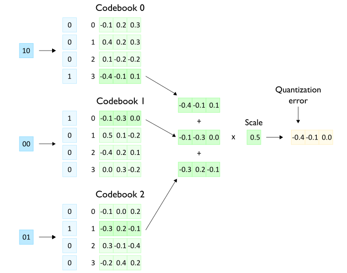
As mentioned previously, at inference time, the matrix multiplication with activations X uses dequantized, native-precision parameters rather than the quantized code vectors. As shown in Figure 2, the dequantization process works by decompressing the code vectors back into one-hot index vectors to retrieve the corresponding codewords from each codebook. These codewords are summed together, then scaled to reproduce the original, half-precision weight values for computation.

Memory footprint of AQLM-quantized models

Most importantly, what is the achieved average number of bits per parameter using AQLM? To store an AQLM-quantized weight matrix, the following information needs to be stored:

• M codebooks, each containing 2^B codewords stored at native 16-bit precision. Each codeword has size (1, g).
• d_out scaling factors, each stored as a 16-bit float
• M code vectors of B bits each to encode each group, of which there are total d_out x d_in/g.

Therefore, the average number of bits per parameter can be calculated with the following formula:

It should be noted that the formula above calculates the average bits per parameter for a single weight matrix, i.e. a single layer, not the entire model.

Let’s look at each term’s contribution for different configurations (Table 2) taking Llama-2–70B feed-forward layer as an example :

To understand how each term contributes for different configurations, let’s examine a specific example: the feed-forward layer of the Llama-2–70B model (d_in=8 192 and d_out=28 672). Table 2 shows the breakdown of each term’s contribution across different configurations for this layer.

The scaling factor terms are always negligible in their contribution. The average number of bits per parameter is primarily dictated by the codes encoding each group. The codebook terms generally have a small contribution, unless both B and g are set to relatively high values (as in Scenario D).

Key AQLM quantization parameters

The group size g, number of codebooks M, and codebook size B are hyperparameters in AQLM’s quantization process. Assuming the code terms dominate the average bits per parameter, we can approximate the total as B.M/g. This means multiple combinations of g, M, and B can satisfy the same overall bit budget. To select the optimal configuration, we need to examine how these parameters impact model performance.

Note: The names of AQLM-quantized models follow a XBit-MxB naming scheme such as ISTA-DASLab/gemma-2b-AQLM-2Bit-1×16-hf for the 2-bit quantized version of Gemma-2B using one codebook with 65 536 (2¹⁶) codewords. Knowing the total bit budget, M and B, we can easily derive g.

Regarding latency, the higher the number of codewords, the slower, i.e. the lower the latency speedup. For example, matrix-vector multiplication of the 2-bit 1×16 (65 536 codewords total) Llama-7B model on GPU (Nvidia RTX 3090) shows a x1.31 speedup compared to the FP16 model, whereas the same size 2×8 (512 codewords total) model achieves a x1.57 speedup.

However, decreasing the number of codewords negatively impacts model accuracy. As an example, the paper demonstrates that the 1×16 Llama-7B model (2-bit range) achieves a perplexity score of 6.29 on WikiText2 [5], while the 2×8 variant of the same model scores 7.98 on the same dataset. In comparison, the FP16 version scores 5.12.

Now, considering a fixed total bit budget (e.g. 2 bits) and codebook size B (e.g. B=8), there are multiple valid (M, g) pairs that satisfy the budget constraint. For instance, with B=8, the pairs (1, 4), (2, 8), …, (8, 32), etc. are valid configurations. The paper demonstrates that within a given budget, larger (M, g) values correlate with lower perplexity, i.e. reduced quantization errors, although with diminishing returns. This reveals a latency-accuracy tradeoff — higher M improves accuracy but also increases latency.

Note: For many quantization methods, the average bits per parameter is dictated by the precision used to store parameters, such as INT8, INT4, INT3, etc. This only allows a few discrete average bits sizes. In contrast, AQLM provides much more flexibility — by adjusting the g, M, and B hyperparameters, a wider range of average bits can be achieved with finer granularity (as shown in Table 3).

Note: Leaving model accuracy aside, it is likely that not all configurations are equally efficient. For instance, if the value of B is not a multiple of 8, then each stored code does not utilize all the bits across the bytes needed to represent it

The AQLM quantization procedure

In the previous section, we assumed the codebooks and codes were already learned in order to demonstrate how AQLM builds a compressed representation. In practice, quantizing a model with AQLM involves learning these codebooks. Once the codebooks have been learned, compressing a weight matrix using the process described above is straightforward.

For an input half-precision weight matrix W, the AQLM quantization process learns: M codebooks C, d_out scaling factors s, and for each group, M code vectors b . These are learned by minimizing the following loss function:

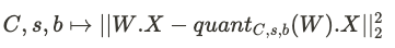
To learn the codebooks and the codes, calibration data (i.e. training data) is required. The authors use a few hundred 4096-length sequences from the RedPajama-v1 dataset [10] as calibration data. Performance is measured by evaluating perplexity on the WikiText2 [5] and C4 [6] datasets, which serve as validation sets.

Looking at technicalities of this particular training would take us too far into the peculiarities of codebook learning. We will just cover the AQLM training (and therefore quantization) procedure main steps.

The AQLM algorithm actually applies to each Transformer decoder block. For a given decoder block, quantization is a two-step process:

1. Codebooks, scaling factors and codes are learned for each linear layer in the block. In each case, the loss function minimization occurs in two stages: 1. The codes are learned first using the initialized codebooks and scaling factors. The codebooks here are fixed, initialized with a residual k-means approach. 2. With the codes learned from the first stage remaining fixed, the codebooks and scaling factors are then updated starting from their initialized values.
2. After quantizing each linear layer in a decoder block, the block’s codebooks, scaling factors, and non-quantized parameters (like normalization layer scales/biases) undergo further fine-tuning. The codes remain frozen at this stage. This fine-tuning uses input and output activations recorded before quantization and allows joint optimization of the parameters across layers. Optimizing jointly accounts for interactions between quantization errors across layers, which is important at very low bitrates where quantization errors are relatively larger.

Pareto optimality

The AQLM authors claim to have pushed the Pareto frontier for the tradeoff between model accuracy (measured by perplexity for example) and memory footprint below 3 bits per weight for the first time. While an important achievement, what does this milestone represent?

Pareto optimality refers to an efficient state where one metric cannot be improved without negatively impacting another metric. For example, consider a system described by two desirable characteristics. A Pareto-optimal state is one where there exists no modification that could improve one characteristic without worsening the other. Conversely, if a change could positively affect one characteristic at no cost to the other, that would be considered Pareto-inefficient, as a more optimal state is possible. The Pareto frontier plots all such Pareto-optimal states.

When applied to model quantization, each model variant (quantized or full-precision) represents a state described by its accuracy and memory footprint. The Pareto frontier comprises the set of (usually quantized) models with the optimal tradeoff between accuracy and size. On this frontier, there exists no way to further compress model size without losing accuracy, or improve accuracy without increasing memory requirements.

For example, the paper shows Llama-2–13B quantized using AQLM to 2 bits per weight achieves 5.65 perplexity, while 4-bit AQLM quantization of Llama-2–7B achieves 5.21 perplexity. Both occupy ~1.7GB, but the 2-bit model has worse accuracy. Therefore at this footprint, the 4-bit model is more efficient — higher accuracy for the same 1.7GB size.

How is that possible? These Pareto efficiency limitations stem from the difficulty quantization techniques face in avoiding substantial accuracy losses at extremely low bit-per-parameter values.

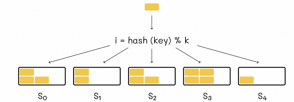
If we assume all quantization techniques could perfectly preserve model accuracy, then each time a new technique achieves higher compression, the Pareto frontier would simply shift to include only models quantized using that latest technique (Figure 3).

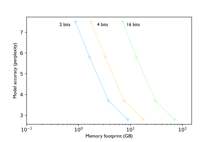
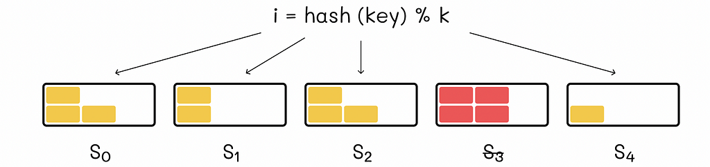
However, because quantization leads to losses in model accuracy, achieving higher compression does not necessarily mean reaching the Pareto frontier if the accuracy loss is too great compared to other existing techniques (Figure 4).

Pushing the Pareto frontier below 3 bits per weight means that existing sub-3-bit quantized models were not Pareto optimal — for a given model memory footprint, accuracy was not maximized. The authors determine 2.5 bits as the optimal rate for the Llama-2 family with AQLM. In other words, Llama-2 models that are quantized to use an average of 2.5 bits per parameter using AQLM sit on the Pareto frontier.

Conclusion

In this post, we introduced AQLM, a new quantization algorithm that applies Multi-Codebook Quantization (MCQ) to large language models for the first time. AQLM sets a new state-of-the-art for model compression in the 2-bit per parameter range and achieves Pareto optimality with sub-3-bit models for the first time.

With its groundbreaking compression rates and maintenance of accuracy, AQLM represents a major step forward in deploying large language models efficiently and making large language models more accessible to consumer hardware and mobile devices.

AQLM is already supported by the HuggingFace Transformers and PEFT libraries, making it easy for developers to leverage AQLM’s advantages!

[1]: V. Egiazarian et al., Extreme Compression of Large Language Models via Additive Quantization (2024), arXiv preprint arXiv:2401.06118

[2]: E. Frantar et al., GPTQ: Accurate Post-Training Quantization for Generative Pre-trained Transformers (2022), ICLR 2023

[3]: J. Chee et al., QuIP: 2-Bit Quantization of Large Language Models With Guarantees (2023), NeurIPS 2023 spotlight

[4]: A. Tseng, QuIP#: Even Better LLM Quantization with Hadamard Incoherence and Lattice Codebooks (2024), arXiv preprint arXiv:2402.04396

[5]: S. Merity et al., Pointer Sentinel Mixture Models (2016), ICLR 2017 Poster

[6]: C. Raffel et al., Exploring the Limits of Transfer Learning with a Unified Text-to-Text Transformer (2019), JMLR 2020

[7]: K. Sagaguchi et al., WinoGrande: An Adversarial Winograd Schema Challenge at Scale (2021), ACM 2021

[8]: R. Zellers et al., HellaSwag: Can a Machine Really Finish Your Sentence? (2019), ACL 2019

[9]: T. Dettmers et al., SpQR: A Sparse-Quantized Representation for Near-Lossless LLM Weight Compression (2023), arXiv preprint arXiv:2306.03078

[10]: Together Computer, RedPajama: an Open Dataset for Training Large Language Models (2023), https://github.com/togethercomputer/RedPajama-Data

The AQLM Quantization Algorithm, Explained was originally published in Towards Data Science on Medium, where people are continuing the conversation by highlighting and responding to this story.

Layman’s guide to appreciating the concept of association

Recently I’ve been working on a project that aims to screen pairs of variables in the stock market, and see how they show enough correlation potential for us to deep-dive and research further.

Throughout my research, I’ve chanced upon many different methodologies; from the humble Spearman’s/Pearson linear correlation, to the more advanced non-linear methods using Time-Delay Embeddings and even Machine Learning techniques.

And that was when I chanced upon this robust and probabilistic concept known as Mutual Information that helps one to measure the level of association/dependence between two variables. This serves as a good Step 0 tool for model development or associative studies.

Scouring the web to understand further, I’ve realized that while there were excellent mathematical and statistical explanations, there weren’t many traces of intuitive insights on how and why Mutual Information works.

And therefore, here we are,

Welcome to my attempt at helping you break down and appreciate this statistical concept!

The Textbook Definition

Mutual Information is a measure of how much “information” you can get of one variable by observing another variable

I’m sure you’ve seen the above statement, or variants of it, throughout your own research. But what exactly is this “information” that they are talking about? How does it tell me that two variables are associated/dependent?

The definition becomes even more daunting when you look at the formulation:

Fret not! Let’s get into breaking down this concept into digestible chunks using a case study.

“Do people really use umbrellas only when it rains?”

said Bob, your drunk friend during a night out of festivities.

He insists that people carry umbrella only when they feel like it, and not because they need it to shelter them from the rain.

You think that that statement is ludicrous! It challenged every observation you made growing up; every notion of logic within your bones.

You decided to stalk Bob and observe him over the next 5 days during his vacation in tropical Singapore. You want to see if he really walks the talk and lives true to his bodacious claims.

You decide to do so using the concept of Mutual Information.

Bob vs Mutual Information

We can break down the Mutual Information formula into the following parts:

The x, X and y, Y

x and y are the individual observations/values that we see in our data. X and Y are just the set of these individual values. A good example would be as follows:

And assuming we have 5 days of observations of Bob in this exact sequence:

Individual/Marginal Probability

These are just the simple probability of observing a particular x or y in their respective sets of possible X and Y values.

Take x = 1 as an example: the probability is simply 0.4 (Bob carried an umbrella 2 out of 5 days of his vacation).

Joint Probability

This is the probability of observing a particular x and y from the joint probability of (X, Y). The joint probability (X, Y) is simply just the set of paired observations. We pair them up according to their index.

In our case with Bob, we pair the observations up based on which day they occurred.

You may be tempted to jump to a conclusion after looking at the pairs:

Since there are equal-value pairs occurring 80% of the time, it clearly means that people carry umbrellas BECAUSE it is raining!

Well I’m here to play the devil’s advocate and say that that may just be a freakish coincidence:

If the chance of rain is very low in Singapore, and, independently, the likelihood of Bob carrying umbrella is also equally low (because he hates holding extra stuff), can you see that the odds of having (0,0) paired observations will be very high naturally?

So what can we do to prove that these paired observations are not by coincidence?

Joint Versus Individual Probabilities

We can take the ratio of both probabilities to give us a clue on the “extent of coincidence”.

In the denominator, we take the product of both individual probabilities of a particular x and particular y occurring. Why did we do so?

Peering into the humble coin toss

Recall the first lesson you took in statistics class: calculating the probability of getting 2 heads in 2 tosses of a fair coin.

• 1st Toss [ p(x) ]: There’s a 50% chance of getting heads
• 2nd Toss [ p(y) ]: There’s still a 50% chance of getting heads, since the outcome is independent of what happened in the 1st toss
• The above 2 tosses make up your individual probabilities
• Therefore, the theoretical probability of getting both heads in 2 independent tosses is 0.5 * 0.5 = 0.25 ( p(x).p(y) )

And if you actually do maybe 100 sets of that double-coin-toss experiment, you’ll likely see that you get the (heads, heads) result 25% of the time. The 100 sets of experiment is actually your (X, Y) joint probability set!

Hence, when you take the ratio of joint versus combined-individual probabilities, you get a value of 1.

This is actually the real expectation for independent events: the joint probability of a specific pair of values occurring is exactly equal to the product of their individual probabilities! Just like what you were taught in fundamental statistics.

Now imagine that your 100-set experiment yielded (heads, heads) 90% of the time. Surely that can’t be a coincidence…

You expected 25% since you know that they are independent events, yet what was observed is an extreme skew of this expectation.

To put this qualitative feeling into numbers, the ratio of probabilities is now a whopping 3.6 (0.9 / 0.25), essentially 3.6x more frequent than we expected.

As such, we start to think that maybe the coin tosses were not independent. Maybe the result of the 1st toss might actually have some unexplained effect on the 2nd toss. Maybe there is some level of association/dependence between 1st and 2nd toss.

That is what Mutual Information tries to tells us!

Expected Value of Observations

For us to be fair to Bob, we should not just look at the times where his claims are wrong, i.e. calculate the ratio of probabilities of (0,0) and (1,1).

We should also calculate the ratio of probabilities for when his claims are correct, i.e. (0,1) and (1,0).

Thereafter, we can aggregate all 4 scenarios in an expected value method, which just means “taking the average”: aggregate up all ratio of probabilities for each observed pair in (X, Y), then divide it by the number of observations.

That is the purpose of these two summation terms. For continuous variables like my stock market example, we will then use integrals instead.

Logarithm of Ratios

Similar to how we calculate the probability of getting 2 consecutive heads for the coin toss, we are also now calculating the additional probability of seeing the 5 pairs that we observed.

For the coin toss, we calculate by multiplying the probabilities of each toss. For Bob, it’s the same: the probabilities have multiplicative effect on each other to give us the sequence that we observed in the joint set.

With logarithms, we turn multiplicative effects into additive ones:

Converting the ratio of probabilities to their logarithmic variants, we can now simply just calculate the expected value as described above using summation of their logarithms.

Feel free to use log-base 2, e, or 10, it does not matter for the purposes of this article.

Putting It All Together

Let’s now prove Bob wrong by calculating the Mutual Information. I will use log-base e (natural logarithm) for my calculations:

So what does the value of 0.223 tell us?

Let’s first assume Bob is right, and that the use of umbrellas are independent from presence of rain:

• We know that the joint probability will exactly equal the product of the individual probabilities.
• Therefore, for every x and y permutation, the ratio of probabilities = 1.
• Taking the logarithm, that equates to 0.
• Thus, the expected value of all permutations (i.e. Mutual Information) is therefore 0.

But since the Mutual Information score that we calculated is non-zero, we can therefore prove to Bob that he is wrong!

Beyond Linear Correlation

Because Mutual Information is a probabilistic measure of association/dependence, it can work for non-linear correlation studies as well!

Take for example two variables X and Y:

Calculating their Mutual Information score, Spearman’s correlation score, and plotting, we get the following:

Relying on Spearman’s correlation alone, we would think that these 2 variables have nothing to do with each other, but we know for a fact that they are deterministically related (based on my formula above)!

The non-zero Mutual Information score hints us to look deeper, albeit not giving us the explicit form of relation.

It is also robust enough to work on strictly linear correlations:

So, if you are ever unsure what kind of correlation you are expecting going into an X-vs-Y analysis, you can try out Mutual Information as a step zero!

My “Layman” Definition of Mutual Information

With the above examples and breakdown, I hope I managed to help you guys get an intuitive understanding what Mutual Information is and how it works.

If it helps you further, I prefer to summarize Mutual Information as follows:

Mutual Information gives us the additional probability of x and y happening at the same time due to other factors above just their chance of co-occurring.

Mutual Information is very useful in areas such as Feature Selection before building your Machine Learning models, and even text association analyses when used with text embeddings. Therefore, it is paramount that we truly know how it works before adopting it for its myriad of uses.

With your newfound intuition and understanding, I believe you will be able to find other pockets of opportunities to apply this versatile concept as I will with my stock market ventures!

An Intuitive View on Mutual Information was originally published in Towards Data Science on Medium, where people are continuing the conversation by highlighting and responding to this story.