Posted by Yun Zhu and Lijuan Liu, Software Engineers, Google Research
Large language model (LLM) advancements have led to a new paradigm that unifies various natural language processing (NLP) tasks within an instruction-following framework. This paradigm is exemplified by recent multi-task LLMs, such as T0, FLAN, and OPT-IML. First, multi-task data is gathered with each task following a task-specific template, where each labeled example is converted into an instruction (e.g., “Put the concepts together to form a sentence: ski, mountain, skier”) paired with a corresponding response (e.g., “Skier skis down the mountain“). These instruction-response pairs are used to train the LLM, resulting in a conditional generation model that takes an instruction as input and generates a response. Moreover, multi-task LLMs have exhibited remarkable task-wise generalization capabilities as they can address unseen tasks by understanding and solving brand-new instructions.
The demonstration of the instruction-following pre-training of multi-task LLMs, e.g., FLAN. Pre-training tasks under this paradigm improves the performance for unseen tasks.
Due to the complexity of understanding and solving various tasks solely using instructions, the size of multi-task LLMs typically spans from several billion parameters to hundreds of billions (e.g., FLAN-11B, T0-11B and OPT-IML-175B). As a result, operating such sizable models poses significant challenges because they demand considerable computational power and impose substantial requirements on the memory capacities of GPUs and TPUs, making their training and inference expensive and inefficient. Extensive storage is required to maintain a unique LLM copy for each downstream task. Moreover, the most powerful multi-task LLMs (e.g., FLAN-PaLM-540B) are closed-sourced, making them impossible to be adapted. However, in practical applications, harnessing a single multi-task LLM to manage all conceivable tasks in a zero-shot manner remains difficult, particularly when dealing with complex tasks, personalized tasks and those that cannot be succinctly defined using instructions. On the other hand, the size of downstream training data is usually insufficient to train a model well without incorporating rich prior knowledge. Hence, it is long desired to adapt LLMs with downstream supervision while bypassing storage, memory, and access issues.
Certain parameter-efficient tuning strategies, including prompt tuning and adapters, substantially diminish storage requirements, but they still perform back-propagation through LLM parameters during the tuning process, thereby keeping their memory demands high. Additionally, some in-context learning techniques circumvent parameter tuning by integrating a limited number of supervised examples into the instruction. However, these techniques are constrained by the model’s maximum input length, which permits only a few samples to guide task resolution.
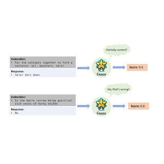
In “Cappy: Outperforming and Boosting Large Multi-Task LMs with a Small Scorer”, presented at NeurIPS 2023, we propose a novel approach that enhances the performance and efficiency of multi-task LLMs. We introduce a lightweight pre-trained scorer, Cappy, based on continual pre-training on top of RoBERTa with merely 360 million parameters. Cappy takes in an instruction and a candidate response as input, and produces a score between 0 and 1, indicating an estimated correctness of the response with respect to the instruction. Cappy functions either independently on classification tasks or serves as an auxiliary component for LLMs, boosting their performance. Moreover, Cappy efficiently enables downstream supervision without requiring any finetuning, which avoids the need for back-propagation through LLM parameters and reduces memory requirements. Finally, adaptation with Cappy doesn’t require access to LLM parameters as it is compatible with closed-source multi-task LLMs, such as those only accessible via WebAPIs.
Cappy takes an instruction and response pair as input and outputs a score ranging from 0 to 1, indicating an estimation of the correctness of the response with respect to the instruction.
Pre-training
We begin with the same dataset collection, which includes 39 diverse datasets from PromptSource that were used to train T0. This collection encompasses a wide range of task types, such as question answering, sentiment analysis, and summarization. Each dataset is associated with one or more templates that convert each instance from the original datasets into an instruction paired with its ground truth response.
Cappy’s regression modeling requires each pre-training data instance to include an instruction-response pair along with a correctness annotation for the response, so we produce a dataset with correctness annotations that range from 0 to 1. For every instance within a generation task, we leverage an existing multi-task LLM to generate multiple responses by sampling, conditioned on the given instruction. Subsequently, we assign an annotation to the pair formed by the instruction and every response, using the similarity between the response and the ground truth response of the instance. Specifically, we employ Rouge-L, a commonly-used metric for measuring overall multi-task performance that has demonstrated a strong alignment with human evaluation, to calculate this similarity as a form of weak supervision.
As a result, we obtain an effective regression dataset of 160 million instances paired with correctness score annotations. The final Cappy model is the result of continuous pre-training using the regression dataset on top of the RoBERTa model. The pre-training of Cappy is conducted on Google’s TPU-v4, with RedCoast, a lightweight toolkit for automating distributed training.
Data augmentation with a multi-task LLM to construct a weakly supervised regression dataset for Cappy’s pre-training and fine-tuning.
Applying Cappy
Cappy solves practical tasks within a candidate-selection mechanism. More specifically, given an instruction and a set of candidate responses, Cappy produces a score for each candidate response. This is achieved by inputting the instruction alongside each individual response, and then assigning the response with the highest score as its prediction. In classification tasks, all candidate responses are inherently predefined. For example, for an instruction of a sentiment classification task (e.g., “Based on this review, would the user recommend this product?: ‘Stunning even for the non-gamer.’”), the candidate responses are “Yes” or “No”. In such scenarios, Cappy functions independently. On the other hand, in generation tasks, candidate responses are not pre-defined, requiring an existing multi-task LLM to yield the candidate responses. In this case, Cappy serves as an auxiliary component of the multi-task LLM, enhancing its decoding.
Adapting multi-task LLMs with Cappy
When there is available downstream training data, Cappy enables effective and efficient adaptation of multi-task LLMs on downstream tasks. Specifically, we fine-tune Cappy to integrate downstream task information into LLM predictions. This process involves creating a separate regression dataset specific to the downstream training data with the same data annotation process used to construct the pre-training data. As a result, the fine-tuned Cappy collaborates with a multi-task LLM, boosting the LLM’s performance on the downstream task.
In contrast to other LLM tuning strategies, adapting LLMs with Cappy significantly reduces the high demand for device memory as it avoids the need for back-propagation through LLM parameters for downstream tasks. Moreover, Cappy adaptation does not rely on the access to LLM parameters, making it compatible with closed-source multi-task LLMs, such as the ones only accessible via WebAPIs. Compared with in-context learning approaches, which circumvent model tuning by attaching training examples to the instruction prefix, Cappy is not restricted by the LLM’s maximum input length. Thus, Cappy can incorporate an unlimited number of downstream training examples. Cappy can also be applied with other adaptation methods, such as fine-tuning and in-context learning, further boosting their overall performance.
Downstream adaptation comparison between Cappy and approaches that rely on an LLM’s parameters, such as fine-tuning and prompt tuning. Cappy’s application enhances multi-task LLMs.
Results
We assess Cappy’s performance across eleven held-out language understanding classification tasks from PromptSource. We demonstrate that Cappy, with 360M parameters, outperforms OPT-175B and OPT-IML-30B, and matches the accuracy of the best existing multi-task LLMs (T0-11B and OPT-IML-175B). These findings highlight Cappy’s capabilities and parameter efficiency, which can be credited to its scoring-based pre-training strategy that integrates contrastive information by differentiating between high-quality and low-quality responses. On the contrary, previous multi-task LLMs depend exclusively on teacher-forcing training that utilizes only the ground truth responses.
The overall accuracy averaged over eleven test tasks from PromptSource. “RM” refers to a pre-trained RLHF reward model. Cappy matches the best ones among existing multi-task LLMs.
We also examine the adaptation of multi-task LLMs with Cappy on complex tasks from BIG-Bench, a set of manually curated tasks that are considered beyond the capability of many LLMs. We focus on all the 45 generation BIG-Bench tasks, specifically those that do not offer pre-established answer choices. We evaluate the performance using the Rouge-L score (representing the overall similarity between model generations and corresponding ground truths) on every test set, reporting the average score across 45 tests. In this experiment, all variants of FLAN-T5 serve as the backbone LLMs, and the foundational FLAN-T5 models are frozen. These results, shown below, suggest that Cappy enhances the performance of FLAN-T5 models by a large margin, consistently outperforming the most effective baseline achieved through sample selection using self-scoring of the LLM itself.
The averaged Rouge-L score over 45 complex tasks within BIG-Bench. The x-axis refers to FLAN-T5 models of different sizes. Every dashed line represents an approach working on FLAN-T5s. Self-scoring refers to using the cross-entropy of LLM to select responses. Cappy enhances the performance of FLAN-T5 models by a large margin.
Conclusion
We introduce Cappy, a novel approach that enhances the performance and efficiency of multi-task LLMs. In our experiments, we adapt a single LLM to several domains with Cappy. In the future, Cappy as a pre-trained model can potentially be used in other creative ways beyond on single LLMs.
Acknowledgments
Thanks to Bowen Tan, Jindong Chen, Lei Meng, Abhanshu Sharma and Ewa Dominowska for their valuable feedback. We would also like to thank Eric Xing and Zhiting Hu for their suggestions.
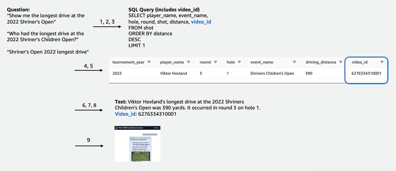
This is a guest post co-written with Scott Gutterman from the PGA TOUR. Generative artificial intelligence (generative AI) has enabled new possibilities for building intelligent systems. Recent improvements in Generative AI based large language models (LLMs) have enabled their use in a variety of applications surrounding information retrieval. Given the data sources, LLMs provided tools […]
In the world of software development, code review and approval are important processes for ensuring the quality, security, and functionality of the software being developed. However, managers tasked with overseeing these critical processes often face numerous challenges, such as the following: Lack of technical expertise – Managers may not have an in-depth technical understanding of […]
Generative AI applications driven by foundational models (FMs) are enabling organizations with significant business value in customer experience, productivity, process optimization, and innovations. However, adoption of these FMs involves addressing some key challenges, including quality output, data privacy, security, integration with organization data, cost, and skills to deliver. In this post, we explore different approaches […]
Note: The code used in this article utilizes three custom scripts, data_cleaning, data_review, and , eda, that can be accessed through a public GitHub repository.
It is like a stretchable fishing net that retains ‘all the big fish’ Zou & Hastie (2005) p. 302
Background
Linear regression is a commonly used teaching tool in data science and, under the appropriate conditions (e.g., linear relationship between the independent and dependent variables, absence of multicollinearity), it can be an effective method for predicting a response. However, in some scenarios (e.g., when the model’s structure becomes complex), its use can be problematic.
To address some of the algorithm’s limitations, penalization or regularization techniques have been suggested [1]. Two popular methods of regularization are ridge and lasso regression, but choosing between these methods can be difficult for those new to the field of data science.
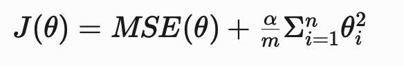
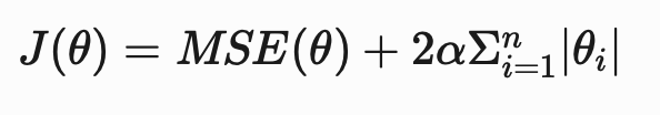
One approach to choosing between ridge and lasso regression is to examine the relevancy of the features to the response variable [2]. When the majority of features in the model are relevant (i.e., contribute to the predictive power of the model), the ridge regression penalty (or L2 penalty) should be added to linear regression.
When the ridge regression penalty is added, the cost function of the model is:
Image by the author
θ = the vector of parameters or coefficients of the model
α = the overall strength of the regularization
m = the number of training examples
n = the number of features in the dataset
When the majority of features are irrelevant (i.e., do not contribute to the predictive power of the model), the lasso regression penalty (or L1 penalty) should be added to linear regression.
When the lasso regression penalty is added, the cost function of the model is:
Image by the author
Relevancy can be determined through manual review or cross validation; however, when working with several features, the process becomes time consuming and computationally expensive.
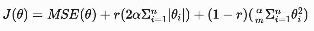
An efficient and flexible solution to this issue is using elastic net regression, which combines the ridge and lasso penalties.
The cost function for elastic net regression is:
Image by the author
r = the mixing ratio between ridge and lasso regression.
When r is 1, only the lasso penalty is used and when r is 0 , only the ridge penalty is used. When r is a value between 0 and 1, a mixture of the penalties is used.
In addition to being well-suited for datasets with several features, elastic net regression has other attributes that make it an appealing tool for data scientists [1]:
Automatic selection of relevant features, which results in parsimonious models that are easy to interpret
Continuous shrinkage, which gradually reduces the coefficients of less relevant features towards zero (opposed to an immediate reduction to zero)
Ability to select groups of correlated features, instead of selecting one feature from the group arbitrarily
Due to its utility and flexibility, Zou and Hastie (2005) compared the model to a “…stretchable fishing net that retains all the big fish.” (p. 302), where big fish are analogous to relevant features.
Now that we have some background, we can move forward to implementing elastic net regression on a real dataset.
Implementation
A great resource for data is the University of California at Irvine’s Machine Learning Repository (UCI ML Repo). For the tutorial, we’ll use the Wine Quality Dataset [3], which is licensed under a Creative Commons Attribution 4.0 International license.
The function displayed below can be used to obtain datasets and variable information from the UCI ML Repo by entering the identification number as the parameter of the function.
pip install ucimlrepo # unless already installed
from ucimlrepo import fetch_ucirepo import pandas as pd
def fetch_uci_data(id): """ Function to return features datasets from the UCI ML Repository.
Parameters ---------- id: int Identifying number for the dataset
Returns ---------- df: df Dataframe with features and response variable """ dataset = fetch_ucirepo(id=id)
description units missing_values 0 None None no 1 None None no 2 None None no 3 None None no 4 None None no 5 None None no 6 None None no 7 None None no 8 None None no 9 None None no 10 None None no 11 score between 0 and 10 None no 12 red or white None no
Based on the variable information, we can see that there are 11 “features”, 1 “target”, and 1 “other” variables in the dataset. This is interesting information — if we had extracted the data without the variable information, we may not have known that there were data available on the family (or color) of wine. At this time, we won’t be incorporating the “color” variable into the model, but it’s nice to know it’s there for future iterations of the project.
The “description” column in the variable information suggests that the “quality” variable is categorical. The data are likely ordinal, meaning they have a hierarchical structure but the intervals between the data are not guaranteed to be equal or known. In practical terms, it means a wine rated as 4 is not twice as good as a wine rated as 2. To address this issue, we’ll convert the data to the proper data-type.
df['quality'] = df['quality'].astype('category')
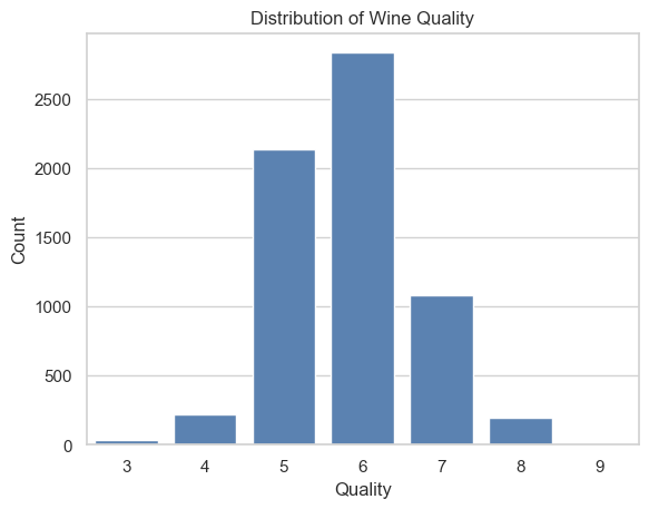
To gain a better understanding of the data, we can use the countplot() method from the seaborn package to visualize the distribution of the “quality” variable.
import seaborn as sns
import matplotlib.pyplot as plt

sns.set_theme(style='whitegrid') # optional

sns.countplot(data=df, x='quality')
plt.title('Distribution of Wine Quality')
plt.xlabel('Quality')
plt.ylabel('Count')
plt.show()
Image by the author
When conducting an exploratory data analysis, creating histograms for numeric features is beneficial. Additionally, grouping the variables by a categorical variable can provide new insights. The best option for grouping the data is “quality”. However, given there are 7 groups of quality, the plots could become difficult to read. To simplify grouping, we can create a new feature, “rating”, that organizes the data on “quality” into three categories: low, medium, and high.
def categorize_quality(value):
 if 0 <= value <= 3:
    return 0 # low rating
 elif 4 <= value <= 6:
    return 1 # medium rating
 else:
    return # high rating

# Create new column for 'rating' data
df['rating'] = df['quality'].apply(categorize_quality)
To determine how many wines are each group, we can use the following code:
Based on the output of the code, we can see that the majority of wines are categorized as “medium”.
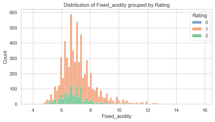
Now, we can plot histograms of the numeric features groups by “rating”. To plot the histogram we’ll need to use the gen_histograms_by_category() method from the eda script in the GitHub repository shared at the beginning of the article.
import eda

eda.gen_histograms_by_category(df, 'rating')
Image by the author
Above is one of the plots generated by the method. A review of the plot indicates there is some skew in the data. To gain a more precise measure of skew, along with other statistics, we can use the get_statistics() method from the data_review script.
Consistent with the histogram, the feature labeled “fixed_acidity” has a skewness of 1.72 indicating significant right-skewness.
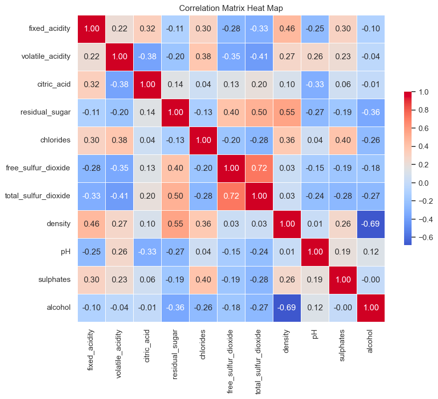
To determine if there are correlations between the variables, we can use another function from the eda script.
eda.gen_corr_matrix_hmap(df)
Image by the author
Although there a few moderate and strong relationships between features, elastic net regression performs well with correlated variables, therefore, no action is required [2].
Data Cleaning
For the elastic net regression algorithm to run correctly, the numeric data must be scaled and the categorical variables must be encoded.
To clean the data, we’ll take the following steps:
Scale the data using the the scale_data() method from the the data_cleaning script
Encode the “quality” and “rating” variables using the the get_dummies() method from pandas
Separate the features (i.e., X) and response variable (i.e., y) using the separate_data() method
Split the data into train and test sets using train_test_split()
from sklearn.model_selection import train_test_split from data_cleaning import scale_data, separate_data
# Separate features and response variable (i.e., 'alcohol') X, y = separate_data(df_encoded, 'alcohol')
# Create test and train sets X_train, X_test, y_train, y_test = train_test_split(X, y, test_size =0.2, random_state=0)
Model Building and Evaluation
To train the model, we’ll use ElasticNetCV() which has two parameters, alpha and l1_ratio, and built-in cross validation. The alpha parameter determines the strength of the regularization applied to the model and l1_ratio determines the mix of the lasso and ridge penalty (it is equivalent to the variable r that was reviewed in the Background section).
When l1_ratio is set to a value of 0, the ridge regression penalty is used.
When l1_ratio is set to a value of 1, the lasso regression penalty is used.
When l1_ratio is set to a value between 0 and 1, a mixture of both penalties are used.
Choosing values for alpha and l1_ratio can be challenging; however, the task is made easier through the use of cross validation, which is built into ElasticNetCV(). To make the process easier, you don’t have to provide a list of values from alpha and l1_ratio — you can let the method do the heavy lifting.
from sklearn.linear_model import ElasticNet, ElasticNetCV
# Build the model elastic_net_cv = ElasticNetCV(cv=5, random_state=1)
# Train the model elastic_net_cv.fit(X_train, y_train)
Mean Squared Error: 0.2999434011721803
R-squared value: 0.7142939720612289
Conclusion
Based on the evaluation metrics, the model performs moderately well. However, its performance could be enhanced through some additional steps, like detecting and removing outliers, additional feature engineering, and providing a specific set of values for alpha and l1_ratio in ElasticNetCV(). Unfortunately, those steps are beyond the scope of this simple tutorial; however, they may provide some ideas for how this project could be improved by others.
Thank you for taking the time to read this article. If you have any questions or feedback, please leave a comment.
References
[1] H. Zou & T. Hastie, Regularization and Variable Selection Via the Elastic Net, Journal of the Royal Statistical Society Series B: Statistical Methodology, Volume 67, Issue 2, April 2005, Pages 301–320, https://doi.org/10.1111/j.1467-9868.2005.00503.x
[2] A. Géron, Hands-On Machine Learning with Scikit-Learn, Keras & Tensorflow: Concepts, Tools, and Techniques to Build Intelligent Systems (2021), O’Reilly.
[3] P. Cortez, A. Cerdeira, F. Almeida, T. Matos, & Reis,J.. (2009). Wine Quality. UCI Machine Learning Repository. https://doi.org/10.24432/C56S3T.
The EU AI Act just passed the European Parliament. You might think, “I’m not in the EU, whatever,” but trust me, this is actually more important to data scientists and individuals around the world than you might think. The EU AI Act is a major move to regulate and manage the use of certain machine learning models in the EU or that affect EU citizens, and it contains some strict rules and serious penalties for violation.
This law has a lot of discussion about risk, and this means risk to the health, safety, and fundamental rights of EU citizens. It’s not just the risk of some kind of theoretical AI apocalypse, it’s about the day to day risk that real people’s lives are made worse in some way by the model you’re building or the product you’re selling. If you’re familiar with many debates about AI ethics today, this should sound familiar. Embedded discrimination and violation of people’s rights, as well as harm to people’s health and safety, are serious issues facing the current crop of AI products and companies, and this law is the EU’s first effort to protect people.
Defining AI
Regular readers know that I always want “AI” to be well defined, and am annoyed when it’s too vague. In this case, the Act defines “AI” as follows:
A machine-based system designed to operate with varying levels of autonomy that may exhibit adaptiveness after deployment and that, for explicit or implicit objectives, infers from the input it receives, how to generate outputs such as predictions, content, recommendations or decisions that can influence physical or virtual environments.
So, what does this really mean? My interpretation is that machine learning models that produce outputs that are used to influence the world (especially people’s physical or digital conditions) fall under this definition. It doesn’t have to adapt live or retrain automatically, although if it does that’s covered.
But if you’re building ML models that are used to do things like…
decide on people’s risk levels, such as credit risk, rule or lawbreaking risk, etc
determine what content people online are shown in a feed, or in ads
differentiate prices shown to different people for the same products
recommend the best treatment, care, or services for people
recommend whether people take certain actions or not
These will all be covered by this law, if your model effects anyone who is a citizen of the EU — and that’s just to name a few examples.
Classifying AI Applications
All AI is not the same, however, and the law acknowledges that. Certain applications of AI are going to be banned entirely, and others subjected to much higher scrutiny and transparency requirements.
Unacceptable Risk AI Systems
These kinds of systems are now called “Unacceptable Risk AI Systems” and are simply not allowed. This part of the law is going into effect first, six months from now.
Behavioral manipulation or deceptive techniques to get people to do things they would otherwise not
Targeting people due to things like age or disability to change their behavior and/or exploit them
Biometric categorization systems, to try to classify people according to highly sensitive traits
Personality characteristic assessments leading to social scoring or differential treatment
“Real-time” biometric identification for law enforcement outside of a select set of use cases (targeted search for missing or abducted persons, imminent threat to life or safety/terrorism, or prosecution of a specific crime)
Predictive policing (predicting that people are going to commit crime in the future)
Broad facial recognition/biometric scanning or data scraping
Emotion inferring systems in education or work without a medical or safety purpose
This means, for example, you can’t build (or be forced to submit to) a screening that is meant to determine whether you’re “happy” enough to get a retail job. Facial recognition is being restricted to only select, targeted, specific situations. (Clearview AI is definitely an example of that.) Predictive policing, something I worked on in academia early in my career and now very much regret, is out.
The “biometric categorization” point refers to models that group people using risky or sensitive traits like political, religious, philosophical beliefs, sexual orientation, race, and so on. Using AI to try and label people according to these categories is understandably banned under the law.
High Risk AI Systems
This list, on the other hand, covers systems that are not banned, but highly scrutinized. There are specific rules and regulations that will cover all these systems, which are described below.
AI in medical devices
AI in vehicles
AI in emotion-recognition systems
AI in policing
This is excluding those specific use cases described above. So, emotion-recognition systems might be allowed, but not in the workplace or in education. AI in medical devices and in vehicles are called out as having serious risks or potential risks for health and safety, rightly so, and need to be pursued only with great care.
Other
The other two categories that remain are “Low Risk AI Systems” and “General Purpose AI Models”. General Purpose models are things like GPT-4, or Claude, or Gemini — systems that have very broad use cases and are usually employed within other downstream products. So, GPT-4 by itself isn’t in a high risk or banned category, but the ways you can embed them for use is limited by the other rules described here. You can’t use GPT-4 for predictive policing, but GPT-4 can be used for low risk cases.
Transparency and Scrutiny
So, let’s say you’re working on a high risk AI application, and you want to follow all the rules and get approval to do it. How to begin?
For High Risk AI Systems, you’re going to be responsible for the following:
Maintain and ensure data quality: The data you’re using in your model is your responsibility, so you need to curate it carefully.
Provide documentation and traceability: Where did you get your data, and can you prove it? Can you show your work as to any changes or edits that were made?
Provide transparency: If the public is using your model (think of a chatbot) or a model is part of your product, you have to tell the users that this is the case. No pretending the model is just a real person on the customer service hotline or chat system. This is actually going to apply to all models, even the low risk ones.
Use human oversight: Just saying “the model says…” isn’t going to cut it. Human beings are going to be responsible for what the results of the model say and most importantly, how the results are used.
Protect cybersecurity and robustness: You need to take care to make your model safe against cyberattacks, breaches, and unintentional privacy violations. Your model screwing up due to code bugs or hacked via vulnerabilities you didn’t fix is going to be on you.
Comply with impact assessments: If you’re building a high risk model, you need to do a rigorous assessment of what the impact could be (even if you don’t mean to) on the health, safety, and rights of users or the public.
For public entities, registration in a public EU database: This registry is being created as part of the new law, and filing requirements will apply to “public authorities, agencies, or bodies” — so mainly governmental institutions, not private businesses.
Testing
Another thing the law makes note of is that if you’re working on building a high risk AI solution, you need to have a way to test it to ensure you’re following the guidelines, so there are allowances for testing on regular people once you get informed consent. Those of us from the social sciences will find this pretty familiar — it’s a lot like getting institutional review board approval to run a study.
Effectiveness
The law has a staggered implementation:
In 6 months, the prohibitions on unacceptable risk AI take effect
In 12 months, general purpose AI governance takes effect
In 24 months, all the remaining rules in the law take effect
Note: The law does not cover purely personal, non-professional activities, unless they fall into the prohibited types listed earlier, so your tiny open source side project isn’t likely to be a risk.
If you do one of the prohibited forms of AI described above:
Fines of up to 35 million Euro or, if you’re a business, 7% of your global revenue from the last year (whichever is higher)
Other violation not included in the prohibited set:
Fines of up to 15 million Euro or, if you’re a business, 3% of your global revenue from the last year (whichever is higher)
Lying to authorities about any of these things:
Fines of up to 7.5 million Euro or, if you’re a business, 1% of your global revenue from the last year (whichever is higher)
Note: For small and medium size businesses, including startups, then the fine is whichever of the numbers is lower, not higher.
What Should Data Scientists Do?
If you’re building models and products using AI under the definition in the Act, you should first and foremost familiarize yourself with the law and what it’s requiring. Even if you aren’t affecting EU citizens today, this is likely to have a major impact on the field and you should be aware of it.
Then, watch out for potential violations in your own business or organization. You have some time to find and remedy issues, but the banned forms of AI take effect first. In large businesses, you’re likely going to have a legal team, but don’t assume they are going to take care of all this for you. You are the expert on machine learning, and so you’re a very important part of how the business can detect and avoid violations. You can use the Compliance Checker tool on the EU AI Act website to help you.
There are many forms of AI in use today at businesses and organizations that are not allowed under this new law. I mentioned Clearview AI above, as well as predictive policing. Emotional testing is also a very real thing that people are subjected to during job interview processes (I invite you to google “emotional testing for jobs” and see the onslaught of companies offering to sell this service), as well as high volume facial or other biometric collection. It’s going to be extremely interesting and important for all of us to follow this and see how enforcement goes, once the law takes full effect.
I’d like to take a moment here and say a few words about a dear friend of mine who passed this week after a tough struggle with cancer. Ed Visel, known online as alistaire, was an outstanding data scientist and gave a ton of his time and talent to the broader data science community. If you asked an R question on StackOverflow in the last decade, there’s a good chance he helped you. He was always patient and kind, because having been a self-made data scientist like me, he knew what it was like to learn this stuff the hard way, and never lost that empathy.
Photo by the author
I had the immense good fortune to work with Ed for a few years, and to be his friend for several more. We lost him far too soon, and my ask is that you help a friend or colleague solve a technical problem in his memory. The data science community is going to be a less friendly place without him.
In addition, if you knew Ed, either online or in person, the family has asked for donations to Severson Dells Nature Center, a place that was special to him.
Setting up a Pypi mirror in an AWS private environment with Terraform
How do you install a Python package in your environment if you don’t have any internet access? I recently came across this issue when creating an AWS Sagemaker Studio environment for my team on AWS.
Building an AWS private environment for Sagemaker
For this particular project, I set up Sagemaker in VPC Only mode with the constraint of keeping the architecture private, which means creating a VPC and private subnets, but no access to the internet.
So all network communications, including application communication with AWS APIs, must go through VPC Endpoint interfaces. This allows for keeping connection secured as data sent and received will never go through the internet using the AWS network backbone instead.
It is particularly suited for limiting exposure to security risks, more particularly when you’re processing personal information, or must comply with some security standards.
Accessing the Pypi package repository from AWS Sagemaker
In my team, Data Scientists use Python as a primary language and sometimes need Python packages that are not provided in Sagemaker’s pre-built Python images, so I’ll focus on this use case. Fortunately, the solution is also working for other languages and repositories like npm.
Your users will typically try to install whatever package they need via pip command. But, as no internet access is allowed, this command will fail because pip won’t be able to contact Pypi.org servers.
Opening internet
One option is to open access to the internet and allow outbound HTTP connections to Fastly CDN IPs used by Pypi.org servers. But, this is not viable in our case as we don’t want any internet connection in the architecture.
This is not a viable option as you’ve to know in advance which Python packages you need to provide, and you’ll somehow have to create public subnets and give the Pypi server mirror access to the internet.
Using AWS Cordeartifact
This is ultimately the solution I came up with and which works in my case.
AWS Codeartifact is the artifact management solution provided by AWS. It is compatible with other AWS services like AWS Service Catalog to control access to resources within an organization.
To use it, you’ll have to create a “domain” which serves as an umbrella to manage access and apply policies across your organization. Then, you’ll have to create a repository that will serve your artifacts to your different applications.
Also, one repository can have upstream repositories. So, if a Python package is not available in the target repository, the demand will be transmitted to the upstream repository to be fulfilled.
More precisely, this workflow takes into account package versions. Official documentation provides a detailed workflow:
If my_repo contains the requested package version, it is returned to the client.
If my_repo does not contain the requested package version, CodeArtifact looks for it in my_repo’s upstream repositories. If the package version is found, a reference to it is copied to my_repo, and the package version is returned to the client.
If neither my_repo nor its upstream repositories contain the package version, an HTTP 404 Not Found response is returned to the client.
Cool right? It will even cache the package version for future requests.
This is precisely the strategy we are going to use, as AWS Codeartifact allows us to define a repository that has an external connection like Pypi as an upstream repository.
Creating AWS Codeartifact resources with Terraform
As AWS Codeartifact is an AWS service, you can easily create a VPC endpoint in your environment VPC to connect to it.
Note: I’m using Terraform v1.6.4 and aws provider v5.38.0
locals { region = "us-east-1" }
resource "aws_security_group" "vpce_sg" { name = "AllowTLS" description = "Allow TLS inbound traffic and all outbound traffic" vpc_id = aws_vpc.your_vpc.id
Then, you’ll have to create the different resources needed for Codeartifact to handle your requests for new Python packages by mirroring Pypi: a domain, a Pypi repository with an external connection, and a repository that defines Pypi as an upstream repository.
Here it is! You can now set up a Pypi mirror for your private environment easily.
To make things usable, you’ll also have to tell pip commands to direct requests to a specific index. Fortunately, AWS created an API to do the heavy lifting for you. Just add this to your code to make it work:
We use cookies on our website to give you the most relevant experience by remembering your preferences and repeat visits. By clicking “Accept”, you consent to the use of ALL the cookies.
This website uses cookies to improve your experience while you navigate through the website. Out of these, the cookies that are categorized as necessary are stored on your browser as they are essential for the working of basic functionalities of the website. We also use third-party cookies that help us analyze and understand how you use this website. These cookies will be stored in your browser only with your consent. You also have the option to opt-out of these cookies. But opting out of some of these cookies may affect your browsing experience.
Necessary cookies are absolutely essential for the website to function properly. These cookies ensure basic functionalities and security features of the website, anonymously.
Cookie
Duration
Description
cookielawinfo-checkbox-analytics
11 months
This cookie is set by GDPR Cookie Consent plugin. The cookie is used to store the user consent for the cookies in the category "Analytics".
cookielawinfo-checkbox-functional
11 months
The cookie is set by GDPR cookie consent to record the user consent for the cookies in the category "Functional".
cookielawinfo-checkbox-necessary
11 months
This cookie is set by GDPR Cookie Consent plugin. The cookies is used to store the user consent for the cookies in the category "Necessary".
cookielawinfo-checkbox-others
11 months
This cookie is set by GDPR Cookie Consent plugin. The cookie is used to store the user consent for the cookies in the category "Other.
cookielawinfo-checkbox-performance
11 months
This cookie is set by GDPR Cookie Consent plugin. The cookie is used to store the user consent for the cookies in the category "Performance".
viewed_cookie_policy
11 months
The cookie is set by the GDPR Cookie Consent plugin and is used to store whether or not user has consented to the use of cookies. It does not store any personal data.
Functional cookies help to perform certain functionalities like sharing the content of the website on social media platforms, collect feedbacks, and other third-party features.
Performance cookies are used to understand and analyze the key performance indexes of the website which helps in delivering a better user experience for the visitors.
Analytical cookies are used to understand how visitors interact with the website. These cookies help provide information on metrics the number of visitors, bounce rate, traffic source, etc.
Advertisement cookies are used to provide visitors with relevant ads and marketing campaigns. These cookies track visitors across websites and collect information to provide customized ads.