In today’s landscape of one-on-one customer interactions for placing orders, the prevailing practice continues to rely on human attendants, even in settings like drive-thru coffee shops and fast-food establishments. This traditional approach poses several challenges: it heavily depends on manual processes, struggles to efficiently scale with increasing customer demands, introduces the potential for human errors, […]
Quantum Machine Learning (QML) represents a fascinating convergence of quantum computing and machine learning technologies. With quantum computing’s potential in mathematics and data processing with complex structure, QML could revolutionize areas like drug discovery, finance, and beyond. This blog delves into the innovative realms of quantum neural networks (QNNs) and quantum kernel techniques, showcasing their unique capabilities through practical Python examples. The blog will not detail the mathematical concepts. For more information do not hesitate to read my latest book Machine Learning Theory and Applications: Hands-on Use Cases with Python on Classical and Quantum Machines, Wiley, 2024.
Quantum kernel methods, introduce a quantum-enhanced way of processing data. By mapping classical data into quantum feature space, these methods utilize the superposition and entanglement properties of quantum mechanics to perform classifications or regression tasks. The use of quantum kernel estimator and quantum variational classifier examples illustrates the practical application of these concepts. QNNs, leveraging quantum states for computation, offer a novel approach to neural network architecture. The Qiskit framework facilitates the implementation of both quantum kernel methods and QNNs, enabling the exploration of quantum algorithms’ efficiency in learning and pattern recognition.
Incorporating Python code examples, this blog aims to provide comprehensive code examples of QML for readers to explore its promising applications, and the challenges it faces. Through these examples, readers can start practicing and gain an appreciation for the transformative potential of quantum computing in machine learning and the exciting possibilities that lie ahead.
First, install qiskit
We will use the open-source SDK Qiskit (https://qiskit.org) which allows working with quantum computers. Qiskit supports Python version 3.6 or later.
In our environment, we can install Qiskit with pip:
pip install qiskit
We can also install qiskit-machine-learning using pip:
To run our code, we can use either simulators or real hardware even if I strongly recommend the use of hardware or push the limits of simulators to improve research in this field. While studying the Qiskit documentation, you will encounter references to the Qiskit Runtime primitives, which serve as implementations of the Sampler and Estimator interfaces found in the qiskit.primitives module. These interfaces facilitate the seamless interchangeability of primitive implementations with minimal code modifications. The initial release of Qiskit Runtime comprises two essential primitives:
Sampler: This primitive generates quasi-probabilities based on input circuits.
Estimator: This primitive calculates expectation values derived from input circuits and observables.
Venturing into quantum approaches for supervised machine learning poses a novel research direction. Classical machine learning extensively utilizes kernel methods, among which the support vector machine (SVM) for classification stands out for its widespread application.
SVMs, known for their role in binary classification, have increasingly been applied to multiclass problems. The essence of binary SVM involves devising a hyperplane to linearly separate n-dimensional data points into two groups, aiming for an optimal margin that distinctively classifies the data into its respective categories. This hyperplane, effective in either the original feature space or a transformed higher-dimensional kernel space, is selected for its capacity to maximize the separation between classes, which involves an optimization problem to maximize the margin, defined as the distance from the nearest data point to the hyperplane on either side. This leads to the formulation of a maximum-margin classifier. The critical data points on the boundary are termed support vectors, and the margin represents a zone typically devoid of data points. An optimal hyperplane too proximate to the data points, indicating a slender margin, undermines the model’s predictive robustness and generalization capability.
To navigate multiclass SVM challenges, methods like the all-pair strategy, which conducts a binary classification for each pair of classes, have been introduced. Beyond straightforward linear classification, nonlinear classifications can be achieved through the kernel trick. This technique employs a kernel function to elevate inputs into a more expansive, higher-dimensional feature space, facilitating the separation of data that is not linearly separable in the input space. The kernel function essentially performs an inner product in a potentially vast Euclidian space, known as the feature space. The goal of nonlinear SVM is to achieve this separation by mapping data to a higher dimension using a suitable mapping. Selecting an appropriate feature map becomes crucial for data that cannot be addressed by linear methods alone. This is where quantum can jump into it. Quantum kernel methods, blending classical kernel strategies with quantum innovations, carve out new avenues in machine learning. Early quantum kernel approaches have focused on encoding data points into inner products or amplitudes in Hilbert space through quantum feature maps. The complexity of the quantum circuit implementing the feature map scales linearly or polylogarithmically with the dataset size.
Quantum Kernel with ZZFeatureMaps
In this first example, we will use the ZZFeatureMap with linear entanglement, we will repeat the data encoding step two times, and we will use feature reduction with principal component analysis. You can of course use other feature reduction, data rescaling or feature selection techniques to improve the accuracy of your models. We will use the breast cancer dataset that you can find here: https://github.com/xaviervasques/hephaistos/blob/main/data/datasets/breastcancer.csv
Let’s describe the steps of the Python script below. This Python script demonstrates an application of integrating quantum computing techniques with traditional machine learning to classify breast cancer data. It represents a hybrid approach, where quantum-enhanced features are used within a classical machine learning workflow. The goal is to predict breast cancer diagnosis (benign or malignant) based on a set of features extracted from the breast mass characteristics.
The way of doing quantum kernel machine learning is very similar to what we do classically as data scientists. We import the necessary libraries (Pandas, NumPy, scikit-learn) and Qiskit for quantum computing and kernel estimation, we load the data, preprocess the data and separate the data into features (X) and target labels (y). A specific step is the quantum feature mapping. The script sets up a quantum feature map using the ZZFeatureMap from Qiskit, configured with specified parameters for feature dimension, repetitions, and entanglement type. Quantum feature maps are critical for translating classical data into quantum states, enabling the application of quantum computing principles for data analysis. Then, the quantum kernel setup consists in configuring a quantum kernel with a fidelity-based approach. It serves as a new method to compute the similarity between data points in the feature space defined by quantum states and potentially capturing complex patterns. The last step comes back to a classic machine learning pipeline with data rescaling with standard scaler, dimension reduction using principal component analysis and the use of support vector classifier (SVC) which utilizes the quantum kernel for classification. We evaluate the model using 5-fold cross-validation.
Let’s code.
# Import necessary libraries for data manipulation, machine learning, and quantum computing
import pandas as pd
import numpy as np
from sklearn.model_selection import train_test_split
from sklearn.preprocessing import LabelEncoder

# Load the dataset using pandas, specifying the file location and delimiter
breastcancer = './breastcancer.csv'
df = pd.read_csv(breastcancer, delimiter=';')

# Remove the 'id' column as it is not useful for prediction, to simplify the dataset
df = df.drop(["id"], axis=1)

# Separate the dataset into features (X) and target label (y)
y = df['diagnosis']  # Target label: diagnosis
X = df.drop('diagnosis', axis=1)  # Features: all other columns

# Convert the diagnosis string labels into numeric values to be used by machine learning models
label_encoder = LabelEncoder()
y = label_encoder.fit_transform(y)

# Quantum computing sections start here
# Set parameters for the quantum feature map
feature_dimension = 2  # Number of features used in the quantum feature map
reps = 2  # Number of repetitions of the feature map circuit
entanglement = 'linear'  # Type of entanglement in the quantum circuit

# Import quantum feature mapping utilities from Qiskit
from qiskit.circuit.library import ZZFeatureMap
qfm = ZZFeatureMap(feature_dimension=feature_dimension, reps=reps, entanglement=entanglement)

# Set up a local simulator for quantum computation
from qiskit.primitives import Sampler
sampler = Sampler()

# Configure quantum kernel using ZZFeatureMap and a fidelity-based quantum kernel
from qiskit.algorithms.state_fidelities import ComputeUncompute
from qiskit_machine_learning.kernels import FidelityQuantumKernel
fidelity = ComputeUncompute(sampler=sampler)
quantum_zz = FidelityQuantumKernel(fidelity=fidelity, feature_map=qfm)

# Create a machine learning pipeline integrating standard scaler, PCA for dimensionality reduction,
# and a Support Vector Classifier using the quantum kernel
from sklearn.pipeline import make_pipeline
from sklearn.preprocessing import StandardScaler
from sklearn.decomposition import PCA
from sklearn.svm import SVC
pipeline = make_pipeline(StandardScaler(), PCA(n_components=2), SVC(kernel=quantum_zz.evaluate))

# Evaluate the model using cross-validation to assess its performance
from sklearn.model_selection import cross_val_score
cv = cross_val_score(pipeline, X, y, cv=5, n_jobs=1)  # n_jobs=1 specifies that the computation will use 1 CPU
mean_score = np.mean(cv)  # Calculate the mean of the cross-validation scores

# Print the mean cross-validation score to evaluate the model's performance
print(mean_score)
We will obtain a mean score validation score of 0.63.
This code is executed with the local simulator. To run on real hardware, replace the following lines:
# Set up a local simulator for quantum computation
from qiskit.primitives import Sampler
sampler = Sampler()
by
# Import necessary classes from qiskit_ibm_runtime for accessing IBM Quantum services
from qiskit_ibm_runtime import QiskitRuntimeService, Sampler

# Initialize the QiskitRuntimeService with your IBM Quantum credentials
# 'channel', 'token', and 'instance' are placeholders for your actual IBM Quantum account details
service = QiskitRuntimeService(channel='YOUR CHANNEL', token='YOUR TOKEN FROM IBM QUANTUM', instance='YOUR INSTANCE')

# Specify the backend you wish to use. This could be a simulator or an actual quantum computer available through IBM Quantum
# 'quantum_backend' should be replaced with the name of the quantum backend you wish to use
backend = service.backend('quantum_backend')

# Import the Options class to customize the execution of quantum programs
from qiskit_ibm_runtime import Options
options = Options()  # Create an instance of Options

# Set the resilience level. Level 1 typically implies some level of error mitigation or resilience against errors
options.resilience_level = 1

# Set the number of shots, which is the number of times the quantum circuit will be executed to gather statistics
# More shots can lead to more accurate results but take longer to execute
options.execution.shots = 1024

# Set the optimization level for compiling the quantum circuit
# Higher optimization levels attempt to reduce the circuit's complexity, which can improve execution but may take longer to compile
options.optimization_level = 3

# Initialize the Sampler, which is used to run quantum circuits and obtain samples from their measurement outcomes
# The Sampler is configured with the specified backend and options
sampler = Sampler(session=backend, options=options)
Quantum Kernel Training
This part will explore the method of Quantum Kernel Alignment (QKA) for the purpose of binary classification. QKA iteratively adjusts a quantum kernel that’s parameterized to fit a dataset, aiming for the largest possible margin in Support Vector Machines (SVM). For further details on QKA, reference is made to the preprint titled “Covariant quantum kernels for data with group structure.” The Python script below is a comprehensive example of integrating traditional machine learning techniques with quantum computing for the prediction accuracy in classifying breast cancer diagnosis. It employs a dataset of breast cancer characteristics to predict the diagnosis (benign or malignant).
The machine learning pipeline is similar to the one used in the quantum kernel with ZZFeatureMaps section. The difference is that we will constructs a custom quantum circuit, integrating a rotational layer with a ZZFeatureMap, to prepare the quantum state representations of the data. The quantum kernel estimation step utilizes Qiskit primitives and algorithms for optimizing the quantum kernel’s parameters using a quantum kernel trained (QKT) and an optimizer.
Let’s code.
# Import necessary libraries for data manipulation, machine learning, and quantum computing
import pandas as pd
import numpy as np
from sklearn.model_selection import train_test_split
from sklearn.preprocessing import LabelEncoder

# Load the dataset using pandas, specifying the file location and delimiter
breastcancer = './breastcancer.csv'
df = pd.read_csv(breastcancer, delimiter=';')

# Remove the 'id' column as it is not useful for prediction, to simplify the dataset
df = df.drop(["id"], axis=1)

# Reduce the dataframe size by sampling 1/3 of the data
df = df.sample(frac=1/3, random_state=1)  # random_state for reproducibility

# Separate the dataset into features (X) and target label (y)
y = df['diagnosis']  # Target label: diagnosis
X = df.drop('diagnosis', axis=1)  # Features: all other columns

# Convert the diagnosis string labels into numeric values to be used by machine learning models
label_encoder = LabelEncoder()
y = label_encoder.fit_transform(y)

# Quantum computing sections start here
# Set parameters for the quantum feature map
feature_dimension = 2  # Number of features used in the quantum feature map
reps = 2  # Number of repetitions of the feature map circuit
entanglement = 'linear'  # Type of entanglement in the quantum circuit

# Define a custom rotational layer for the quantum feature map
from qiskit import QuantumCircuit
from qiskit.circuit import ParameterVector
training_params = ParameterVector("θ", 1)
fm0 = QuantumCircuit(feature_dimension)
for qubit in range(feature_dimension):
    fm0.ry(training_params[0], qubit)

# Use ZZFeatureMap to represent input data
from qiskit.circuit.library import ZZFeatureMap
fm1 = ZZFeatureMap(feature_dimension=feature_dimension, reps=reps, entanglement=entanglement)

# Compose the custom rotational layer with the ZZFeatureMap to create the feature map
fm = fm0.compose(fm1)

# Initialize the Sampler, a Qiskit primitive for sampling from quantum circuits
from qiskit.primitives import Sampler
sampler = Sampler()

# Set up the ComputeUncompute fidelity object for quantum kernel estimation
from qiskit.algorithms.state_fidelities import ComputeUncompute
from qiskit_machine_learning.kernels import TrainableFidelityQuantumKernel
fidelity = ComputeUncompute(sampler=sampler)

# Instantiate the quantum kernel with the feature map and training parameters
quant_kernel = TrainableFidelityQuantumKernel(fidelity=fidelity, feature_map=fm, training_parameters=training_params)

# Callback class for tracking optimization progress
class QKTCallback:
    # Callback wrapper class
    def __init__(self):
        self._data = [[] for i in range(5)]

    def callback(self, x0, x1=None, x2=None, x3=None, x4=None):
        #Capture callback data for analysis
        for i, x in enumerate([x0, x1, x2, x3, x4]):
            self._data[i].append(x)

    def get_callback_data(self):
        #Get captured callback data
        return self._data

    def clear_callback_data(self):
        #Clear captured callback data
        self._data = [[] for i in range(5)]

# Setup and instantiate the optimizer for the quantum kernel
from qiskit.algorithms.optimizers import SPSA
cb_qkt = QKTCallback()
spsa_opt = SPSA(maxiter=10, callback=cb_qkt.callback, learning_rate=0.01, perturbation=0.05)

# Quantum Kernel Trainer (QKT) for optimizing the kernel parameters
from qiskit_machine_learning.kernels.algorithms import QuantumKernelTrainer
qkt = QuantumKernelTrainer(
    quantum_kernel=quant_kernel, loss="svc_loss", optimizer=spsa_opt, initial_point=[np.pi / 2]
)

# Reduce dimensionality of the data using PCA
from sklearn.decomposition import PCA
pca = PCA(n_components=2)
X_ = pca.fit_transform(X)

# Train the quantum kernel with the reduced dataset
qka_results = qkt.fit(X_, y)
optimized_kernel = qka_results.quantum_kernel

# Use the quantum-enhanced kernel in a Quantum Support Vector Classifier (QSVC)
from qiskit_machine_learning.algorithms import QSVC
from sklearn.pipeline import make_pipeline
from sklearn.preprocessing import StandardScaler
qsvc = QSVC(quantum_kernel=optimized_kernel)
pipeline = make_pipeline(StandardScaler(), PCA(n_components=2), qsvc)

# Evaluate the performance of the model using cross-validation
from sklearn.model_selection import cross_val_score
cv = cross_val_score(pipeline, X, y, cv=5, n_jobs=1)
mean_score = np.mean(cv)

# Print the mean cross-validation score
print(mean_score)
We will obtain the following output: 0.6526315789473685
As you certainly observed, there is time differences in execution between QKT and using a quantum kernel with a predefined feature map like ZZFeatureMap even if we reduced the dataframe size by sampling 1/3 of the data and setting the maximum iteration for SPSA to 10. QKT involves not only the use of a quantum kernel but also the optimization of parameters within the quantum feature map or the kernel itself to improve model performance. This optimization process requires iterative adjustments to the parameters, where each iteration involves running quantum computations to evaluate the performance of the current parameter set. This iterative nature significantly increases computational time. When using a predefined quantum kernel like the ZZFeatureMap, the feature mapping is fixed, and there’s no iterative optimization of quantum parameters involved. The quantum computations are performed to evaluate the kernel between data points, but without the added overhead of adjusting and optimizing quantum circuit parameters. This approach is more straightforward and requires fewer quantum computations, making it faster. Each step of the optimization process in QKT requires evaluating the model’s performance with the current quantum kernel, which depends on the quantum feature map parameters at that step. This means multiple evaluations of the kernel matrix, each of which requires a substantial number of quantum computations.
Quantum Neural Networks
This Python script below incorporates quantum neural networks (QNNs) into a machine learning pipeline. In the script, we need to configure the quantum feature map and ansatz (a quantum circuit structure), construct a quantum circuit by appending the feature map and ansatz to a base quantum circuit (this setup is crucial for creating quantum neural networks that process input data quantum mechanically) and create a QNN using the quantum circuit designed for binary classification. Before coming back to the classic machine learning pipeline with data rescaling, data reduction and model evaluation, we employ a quantum classifier which integrates the QNN with a classical optimization algorithm (COBYLA) for training. A callback function is defined to visualize the optimization process, tracking the objective function value across iterations.
Let’s code.
# Importing essential libraries for handling data, machine learning, and integrating quantum computing
import pandas as pd
import numpy as np
from sklearn.model_selection import train_test_split
from sklearn.preprocessing import LabelEncoder
import matplotlib.pyplot as plt  # For data visualization

# Load and prepare the dataset
breastcancer = './breastcancer.csv'
df = pd.read_csv(breastcancer, delimiter=';')  # Load dataset from CSV file
df = df.drop(["id"], axis=1)  # Remove the 'id' column as it's not necessary for analysis

# Splitting the data into features (X) and the target variable (y)
y = df['diagnosis']  # Target variable: diagnosis result
X = df.drop('diagnosis', axis=1)  # Feature matrix: all data except the diagnosis

# Encoding string labels in 'y' into numerical form for machine learning models
label_encoder = LabelEncoder()
y = label_encoder.fit_transform(y)  # Transform labels to numeric

# Quantum feature map and circuit configuration
feature_dimension = 2  # Dimensionality for the feature map (matches PCA reduction later)
reps = 2  # Number of repetitions of the ansatz circuit for depth
entanglement = 'linear'  # Type of qubit entanglement in the circuit

# Initialize an array to store evaluations of the objective function during optimization
objective_func_vals = []

# Define a callback function for visualization of the optimization process
def callback_graph(weights, obj_func_eval):
    """Updates and saves a plot of the objective function value after each iteration."""
    objective_func_vals.append(obj_func_eval)
    plt.title("Objective function value against iteration")
    plt.xlabel("Iteration")
    plt.ylabel("Objective function value")
    plt.plot(range(len(objective_func_vals)), objective_func_vals)
    plt.savefig('Objective_function_value_against_iteration.png')  # Save plot to file

# Example function not directly used in the main workflow, demonstrating a utility function
def parity(x):
    """Example function to calculate parity of an integer."""
    return "{:b}".format(x).count("1") % 2

# Initializing the quantum sampler from Qiskit
from qiskit.primitives import Sampler
sampler = Sampler()  # Used for sampling from quantum circuits

# Constructing the quantum feature map and ansatz for the quantum circuit
from qiskit.circuit.library import ZZFeatureMap, RealAmplitudes
feature_map = ZZFeatureMap(feature_dimension)
ansatz = RealAmplitudes(feature_dimension, reps=reps)  # Quantum circuit ansatz

# Composing the quantum circuit with the feature map and ansatz
from qiskit import QuantumCircuit
qc = QuantumCircuit(feature_dimension)
qc.append(feature_map, range(feature_dimension))  # Apply feature map to circuit
qc.append(ansatz, range(feature_dimension))  # Apply ansatz to circuit
qc.decompose().draw()  # Draw and decompose circuit for visualization

# Creating a Quantum Neural Network (QNN) using the configured quantum circuit
from qiskit_machine_learning.neural_networks import SamplerQNN
sampler_qnn = SamplerQNN(
    circuit=qc,
    input_params=feature_map.parameters,
    weight_params=ansatz.parameters,
    output_shape=2,  # For binary classification
    sampler=sampler
)

# Configuring the quantum classifier with the COBYLA optimizer
from qiskit.algorithms.optimizers import COBYLA
from qiskit_machine_learning.algorithms.classifiers import NeuralNetworkClassifier
sampler_classifier = NeuralNetworkClassifier(
    neural_network=sampler_qnn, optimizer=COBYLA(maxiter=100), callback=callback_graph)

# Setting up K-Fold Cross Validation to assess model performance
from sklearn.model_selection import KFold
k_fold = KFold(n_splits=5)  # 5-fold cross-validation
score = np.zeros(5)  # Array to store scores for each fold
i = 0  # Index counter for scores array
for indices_train, indices_test in k_fold.split(X):
    X_train, X_test = X.iloc[indices_train], X.iloc[indices_test]
    y_train, y_test = y[indices_train], y[indices_test]

    # Applying PCA to reduce the dimensionality of the dataset to match the quantum feature map
    from sklearn.decomposition import PCA
    pca = PCA(n_components=2)  # Reduce to 2 dimensions for the quantum circuit
    X_train = pca.fit_transform(X_train)  # Transform training set
    X_test = pca.fit_transform(X_test)  # Transform test set

    # Training the quantum classifier with the training set
    sampler_classifier.fit(X_train, y_train)

    # Evaluating the classifier's performance on the test set
    score[i] = sampler_classifier.score(X_test, y_test)  # Store score for this fold
    i += 1  # Increment index for next score

# Calculating and displaying the results of cross-validation
import math
print("Cross-validation scores:", score)
cross_mean = np.mean(score)  # Mean of cross-validation scores
cross_var = np.var(score)  # Variance of scores
cross_std = math.sqrt(cross_var)  # Standard deviation of scores

print("Mean cross-validation score:", cross_mean)
print("Standard deviation of cross-validation scores:", cross_std)
Standard deviation of cross-validation scores: 0.09618163326986424
As we can see, in this specific dataset, QNN doesn’t provide a very good classification score.
Conclusion
This idea of this blog is to make it easy to start using quantum machine learning. Quantum Machine Learning is an emerging field at the intersection of quantum computing and machine learning that holds the potential to revolutionize how we process and analyze vast datasets by leveraging the inherent advantages of quantum mechanics. As we showed in our paper Application of quantum machine learning using quantum kernel algorithms on multiclass neuron M-type classification published in Nature Scientific Report, a crucial aspect of optimizing QML models, including Quantum Neural Networks (QNNs), involves pre-processing techniques such as feature rescaling, feature extraction, and feature selection.
These techniques are not only essential in classical machine learning but also present significant benefits when applied within the quantum computing framework, enhancing the performance and efficiency of quantum machine learning algorithms. In the quantum realm, feature extraction techniques like Principal Component Analysis (PCA) can be quantum-enhanced to reduce the dimensionality of the data while retaining most of its significant information. This reduction is vital for QML models due to the limited number of qubits available on current quantum hardware.
Quantum feature extraction can efficiently map high-dimensional data into a lower-dimensional quantum space, enabling quantum models to process complex datasets with fewer resources. Selecting the most relevant features is also a way for optimizing quantum circuit complexity and resource allocation. In quantum machine learning, feature selection helps in identifying and utilizing the most informative features, reducing the need for extensive quantum resources.
This process not only simplifies the quantum models but also enhances their performance by focusing the computational efforts on the features that contribute the most to the predictive accuracy of the model.
Posted by Mike Schaekermann, Research Scientist, Google Research, and Ivor Horn, Chief Health Equity Officer & Director, Google Core
Health equity is a major societal concern worldwide with disparities having many causes. These sources include limitations in access to healthcare, differences in clinical treatment, and even fundamental differences in the diagnostic technology. In dermatology for example, skin cancer outcomes are worse for populations such as minorities, those with lower socioeconomic status, or individuals with limited healthcare access. While there is great promise in recent advances in machine learning (ML) and artificial intelligence (AI) to help improve healthcare, this transition from research to bedside must be accompanied by a careful understanding of whether and how they impact health equity.
Health equity is defined by public health organizations as fairness of opportunity for everyone to be as healthy as possible. Importantly, equity may be different from equality. For example, people with greater barriers to improving their health may require more or different effort to experience this fair opportunity. Similarly, equity is not fairness as defined in the AI for healthcare literature. Whereas AI fairness often strives for equal performance of the AI technology across different patient populations, this does not center the goal of prioritizing performance with respect to pre-existing health disparities.
Health equity considerations. An intervention (e.g., an ML-based tool, indicated in dark blue) promotes health equity if it helps reduce existing disparities in health outcomes (indicated in lighter blue).
In “Health Equity Assessment of machine Learning performance (HEAL): a framework and dermatology AI model case study”, published in The Lancet eClinicalMedicine, we propose a methodology to quantitatively assess whether ML-based health technologies perform equitably. In other words, does the ML model perform well for those with the worst health outcomes for the condition(s) the model is meant to address? This goal anchors on the principle that health equity should prioritize and measure model performance with respect to disparate health outcomes, which may be due to a number of factors that include structural inequities (e.g., demographic, social, cultural, political, economic, environmental and geographic).
The health equity framework (HEAL)
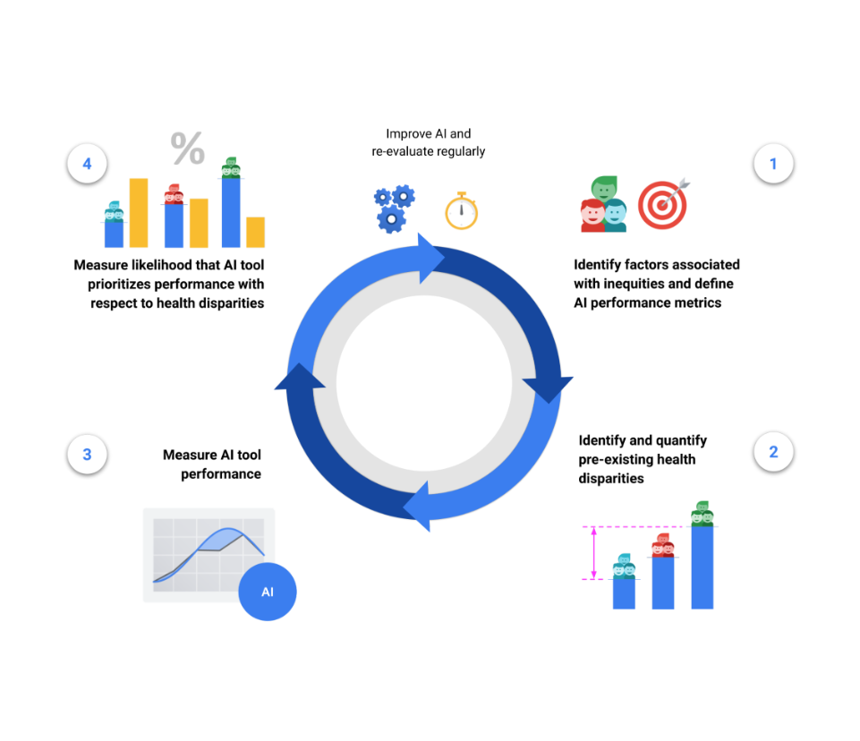
The HEAL framework proposes a 4-step process to estimate the likelihood that an ML-based health technology performs equitably:
Identify factors associated with health inequities and define tool performance metrics,
Identify and quantify pre-existing health disparities,
Measure the performance of the tool for each subpopulation,
Measure the likelihood that the tool prioritizes performance with respect to health disparities.
The final step’s output is termed the HEAL metric, which quantifies how anticorrelated the ML model’s performance is with health disparities. In other words, does the model perform better with populations that have the worse health outcomes?
This 4-step process is designed to inform improvements for making ML model performance more equitable, and is meant to be iterative and re-evaluated on a regular basis. For example, the availability of health outcomes data in step (2) can inform the choice of demographic factors and brackets in step (1), and the framework can be applied again with new datasets, models and populations.
Framework for Health Equity Assessment of machine Learning performance (HEAL). Our guiding principle is to avoid exacerbating health inequities, and these steps help us identify disparities and assess for inequitable model performance to move towards better outcomes for all.
With this work, we take a step towards encouraging explicit assessment of the health equity considerations of AI technologies, and encourage prioritization of efforts during model development to reduce health inequities for subpopulations exposed to structural inequities that can precipitate disparate outcomes. We should note that the present framework does not model causal relationships and, therefore, cannot quantify the actual impact a new technology will have on reducing health outcome disparities. However, the HEAL metric may help identify opportunities for improvement, where the current performance is not prioritized with respect to pre-existing health disparities.
Case study on a dermatology model
As an illustrative case study, we applied the framework to a dermatology model, which utilizes a convolutional neural network similar to that described in prior work. This example dermatology model was trained to classify 288 skin conditions using a development dataset of 29k cases. The input to the model consists of three photos of a skin concern along with demographic information and a brief structured medical history. The output consists of a ranked list of possible matching skin conditions.
Using the HEAL framework, we evaluated this model by assessing whether it prioritized performance with respect to pre-existing health outcomes. The model was designed to predict possible dermatologic conditions (from a list of hundreds) based on photos of a skin concern and patient metadata. Evaluation of the model is done using a top-3 agreement metric, which quantifies how often the top 3 output conditions match the most likely condition as suggested by a dermatologist panel. The HEAL metric is computed via the anticorrelation of this top-3 agreement with health outcome rankings.
We used a dataset of 5,420 teledermatology cases, enriched for diversity in age, sex and race/ethnicity, to retrospectively evaluate the model’s HEAL metric. The dataset consisted of “store-and-forward” cases from patients of 20 years or older from primary care providers in the USA and skin cancer clinics in Australia. Based on a review of the literature, we decided to explore race/ethnicity, sex and age as potential factors of inequity, and used sampling techniques to ensure that our evaluation dataset had sufficient representation of all race/ethnicity, sex and age groups. To quantify pre-existing health outcomes for each subgroup we relied on measurements from publicdatabases endorsed by the World Health Organization, such as Years of Life Lost (YLLs) and Disability-Adjusted Life Years (DALYs; years of life lost plus years lived with disability).
HEAL metric for all dermatologic conditions across race/ethnicity subpopulations, including health outcomes (YLLs per 100,000), model performance (top-3 agreement), and rankings for health outcomes and tool performance. (* Higher is better; measures the likelihood the model performs equitably with respect to the axes in this table.)
HEAL metric for all dermatologic conditions across sexes, including health outcomes (DALYs per 100,000), model performance (top-3 agreement), and rankings for health outcomes and tool performance. (* As above.)
Our analysis estimated that the model was 80.5% likely to perform equitably across race/ethnicity subgroups and 92.1% likely to perform equitably across sexes.
However, while the model was likely to perform equitably across age groups for cancer conditions specifically, we discovered that it had room for improvement across age groups for non-cancer conditions. For example, those 70+ have the poorest health outcomes related to non-cancer skin conditions, yet the model didn’t prioritize performance for this subgroup.
HEAL metrics for all cancer and non-cancer dermatologic conditions across age groups, including health outcomes (DALYs per 100,000), model performance (top-3 agreement), and rankings for health outcomes and tool performance. (* As above.)
Putting things in context
For holistic evaluation, the HEAL metric cannot be employed in isolation. Instead this metric should be contextualized alongside many other factors ranging from computational efficiency and data privacy to ethical values, and aspects that may influence the results (e.g., selection bias or differences in representativeness of the evaluation data across demographic groups).
As an adversarial example, the HEAL metric can be artificially improved by deliberately reducing model performance for the most advantaged subpopulation until performance for that subpopulation is worse than all others. For illustrative purposes, given subpopulations A and B where A has worse health outcomes than B, consider the choice between two models: Model 1 (M1) performs 5% better for subpopulation A than for subpopulation B. Model 2 (M2) performs 5% worse on subpopulation A than B. The HEAL metric would be higher for M1 because it prioritizes performance on a subpopulation with worse outcomes. However, M1 may have absolute performances of just 75% and 70% for subpopulations A and B respectively, while M2 has absolute performances of 75% and 80% for subpopulations A and B respectively. Choosing M1 over M2 would lead to worse overall performance for all subpopulations because some subpopulations are worse-off while no subpopulation is better-off.
Accordingly, the HEAL metric should be used alongside a Pareto condition (discussed further in the paper), which restricts model changes so that outcomes for each subpopulation are either unchanged or improved compared to the status quo, and performance does not worsen for any subpopulation.
The HEAL framework, in its current form, assesses the likelihood that an ML-based model prioritizes performance for subpopulations with respect to pre-existing health disparities for specific subpopulations. This differs from the goal of understanding whether ML will reduce disparities in outcomes across subpopulations in reality. Specifically, modeling improvements in outcomes requires a causal understanding of steps in the care journey that happen both before and after use of any given model. Future research is needed to address this gap.
Conclusion
The HEAL framework enables a quantitative assessment of the likelihood that health AI technologies prioritize performance with respect to health disparities. The case study demonstrates how to apply the framework in the dermatological domain, indicating a high likelihood that model performance is prioritized with respect to health disparities across sex and race/ethnicity, but also revealing the potential for improvements for non-cancer conditions across age. The case study also illustrates limitations in the ability to apply all recommended aspects of the framework (e.g., mapping societal context, availability of data), thus highlighting the complexity of health equity considerations of ML-based tools.
This work is a proposed approach to address a grand challenge for AI and health equity, and may provide a useful evaluation framework not only during model development, but during pre-implementation and real-world monitoring stages, e.g., in the form of health equity dashboards. We hold that the strength of the HEAL framework is in its future application to various AI tools and use cases and its refinement in the process. Finally, we acknowledge that a successful approach towards understanding the impact of AI technologies on health equity needs to be more than a set of metrics. It will require a set of goals agreed upon by a community that represents those who will be most impacted by a model.
Acknowledgements
The research described here is joint work across many teams at Google. We are grateful to all our co-authors: Terry Spitz, Malcolm Pyles, Heather Cole-Lewis, Ellery Wulczyn, Stephen R. Pfohl, Donald Martin, Jr., Ronnachai Jaroensri, Geoff Keeling, Yuan Liu, Stephanie Farquhar, Qinghan Xue, Jenna Lester, Cían Hughes, Patricia Strachan, Fraser Tan, Peggy Bui, Craig H. Mermel, Lily H. Peng, Yossi Matias, Greg S. Corrado, Dale R. Webster, Sunny Virmani, Christopher Semturs, Yun Liu, and Po-Hsuan Cameron Chen. We also thank Lauren Winer, Sami Lachgar, Ting-An Lin, Aaron Loh, Morgan Du, Jenny Rizk, Renee Wong, Ashley Carrick, Preeti Singh, Annisah Um’rani, Jessica Schrouff, Alexander Brown, and Anna Iurchenko for their support of this project.
Traditionally, any natural language processing text classification project would start with gathering instances, defining their respective labels, and training a classification model, such as a logistic regression model, to classify the instances. Currently, the models available in OpenAI can be directly used for classification tasks that would typically require collecting a substantial amount of labeled data to train the model. These pre-trained models can be used for multiple text-processing tasks, including classification, summarization, spell-checking, and keyword identification. We don’t require any labeled data or the need to train a model. Simple, right?
ChatGPT provides a graphical interface for the models implemented by OpenAI. However, what if we want to run those models directly in Python? Well, the available alternative is the OpenAI API, which allows us to access their models from a programming environment. In this article, we will describe with a brief example how we can access the API to detect whether an SMS is spam or not. To accomplish this, we will utilize one of the Open AI models, specifically the GPT-3.5-turbo model.
Creating an Open AI Account
The initial step to access the OpenAI API involves creating an account on OpenAI to obtain the API key required for accessing the models. Upon creating the account, we’ll have $5 of credit at our disposal, which, as we will later observe, will allow us to conduct numerous tests.
In this example, we’ll utilize the free version of OpenAI, which comes with limitations on requests per minute and per day. Adhering to these limits is crucial to avoid Rate Limit Errors. The values for these two parameters are set at 3 requests per minute and 200 per day. While this naturally imposes constraints, particularly for large-scale projects, it suffices for the purposes of this article’s example.
Accessing OpenAI with Python
Once we have created the account, we can access the OpenAI models available for the free version from Python using the OpenAI library. First, we create a function called chat_with_gpt to access the GPT-3.5-turbo model. The input to this function will be the prompt, which we will design later on.
Designing the Prompt
The next step is to create the prompt that we will provide to the GPT-3.5-turbo model. In this particular case, we are interested in two things. Firstly, a value between 0 and 1 indicating the probability of the SMS being spam or not, and secondly, an explanation of the model’s reasoning behind that decision. Additionally, we desire the result in JSON format so that we can later convert it into a dataframe. Below is the template we will use for these predictions.
Reading the SMS Spam Collection Dataset
Now, we need some messages to test how well the OpenAI model predicts whether a message is spam or not. For this purpose, we will use the SMS Spam Collection dataset available on the UCI Machine Learning Repository.
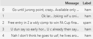
We read the data and convert it into a DataFrame. As observed, the dataset consists of two columns: one containing the messages and the second containing the corresponding labels. ham indicates that the message is not spam, while spam indicates that it is.
Spam Collection dataset (Image created by the author)
Utilizing the GPT-3.5-turbo Model for Spam Detection in Messages
Now, we will use the model to detect whether the messages are spam or not and evaluate how well the pre-trained OpenAI model can predict this problem. As mentioned at the beginning of the article, there are significant limitations regarding the number of requests per minute and per day that we can make with the free version. The dataset contains 5,574 instances, but to test the model, we will only use the first 50 instances. If you have a paid version of OpenAI, you can increase the number of messages tested as the time limitations are much lower.
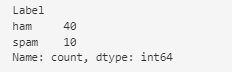
Labels of instances (Image created by the author)
Before making predictions with the model, we have verified that our dataset of 50 instances contains both messages that are spam and messages that are not. In total, there are 40 non-spam messages and 10 spam messages.
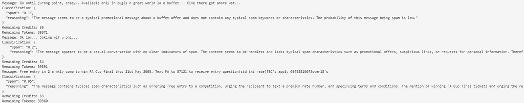
Finally, we proceed to make the prediction. As shown below, we have kept track of the available credits and tokens at all times. Additionally, we have implemented a sleep function in the code for 60 seconds to ensure compliance with the restrictions regarding the number of requests.
The message provided by the model with the prediction has been stored in a variable called prediction. This message is a JSON file with the following structure: { “spam”: “0.1”, “reasoning”: “The message seems to be a typical promotional message about a buffet offer and does not contain any typical spam keywords or characteristics. The probability of this message being spam is low.” }.
Testing output (Image created by the author)
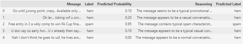
The predictions yield a value between 0 and 1. A value of 0 indicates that the message is not spam, while a value of 1 indicates that it is. To assign the labels, we will use a threshold of 0.5, meaning that a score higher than 0.5 by the model will categorize the message as spam.
Predicted Labels (Image created by the author)
Now, all that’s left is to compare the actual labels with the predicted labels and assess how well the GPT-3.5-turbo model has performed the predictions.
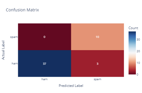
Confusion Matrix (Image created by the author)
Above is the confusion matrix of the model.
For messages that are not spam (ham), the model correctly predicted 37 of them as not spam (true negatives), but misclassified 3 of them as spam (false positives).
For messages that are spam, the model correctly predicted 10 of them as spam (true positives), with no observed false negatives in this case.
The model demonstrates good sensitivity in detecting spam messages, with a few false positives indicating potential areas for improvement in its precision. As shown, the model achieved a 94% accuracy rate, correctly classifying 47 out of 50 instances.
Since we’ve requested the model to provide us with information regarding its reasoning for classifying a message as spam or not, we can examine why it misclassified 3 messages that do not belong to the spam category. Below are the explanations provided by the model:
The message contains unusual language and grammar mistakes commonly associated with spam messages. It also mentions sensitive topics like AIDS, which is a common tactic used in spam messages to evoke emotions and prompt a response. Therefore, there is a high probability of this message being spam.
The message contains suggestive and inappropriate content, which is a common characteristic of spam messages. Additionally, the use of improper grammar and language may indicate that this message is spam. Therefore, the probability of this message being spam is high.
The message contains suggestive content related to personal attributes, which is a common characteristic of spam messages. Additionally, the use of explicit language increases the likelihood of this message being considered spam.
Messages with inappropriate content or numerous spelling errors tend to be classified as spam.
Project Summary
Traditionally, projects requiring text classification began with labeled databases and a model that needed training. The emergence of pre-trained Language Models (LLMs) now offers the possibility of classifying a multitude of texts without the need to train a model beforehand, as these models have already been trained for many use cases. In this article, we have explained how to utilize the OpenAI API to access the GPT-3.5-turbo model and determine whether a set of messages is spam or not. The model was able to classify 94% of the instances correctly, which indicates a high level of accuracy. In the future, it could be worthwhile to evaluate other OpenAI models and explore different prompts that may yield better performance. By the way, the execution of the project only costed $0.007.
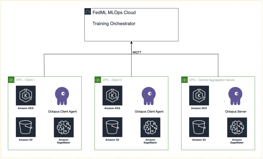
This post is co-written with Chaoyang He, Al Nevarez and Salman Avestimehr from FedML. Many organizations are implementing machine learning (ML) to enhance their business decision-making through automation and the use of large distributed datasets. With increased access to data, ML has the potential to provide unparalleled business insights and opportunities. However, the sharing of […]
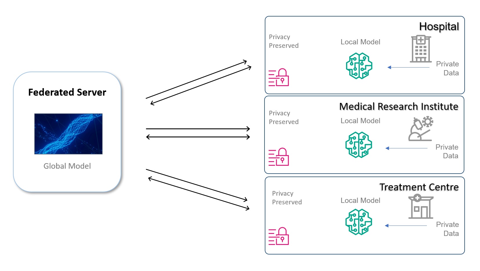
This is a guest blog post written by Nitin Kumar, a Lead Data Scientist at T and T Consulting Services, Inc. In this post, we discuss the value and potential impact of federated learning in the healthcare field. This approach can help heart stroke patients, doctors, and researchers with faster diagnosis, enriched decision-making, and more […]
First-order principles of brain structure for AI assistants
Hello everyone, this article is a written form of a tutorial I conducted two weeks ago with Neurons Lab. If you prefer a narrative walkthrough, you can find the YouTube video here:
As always, you can find the code on GitHub, and here are separate Colab Notebooks:
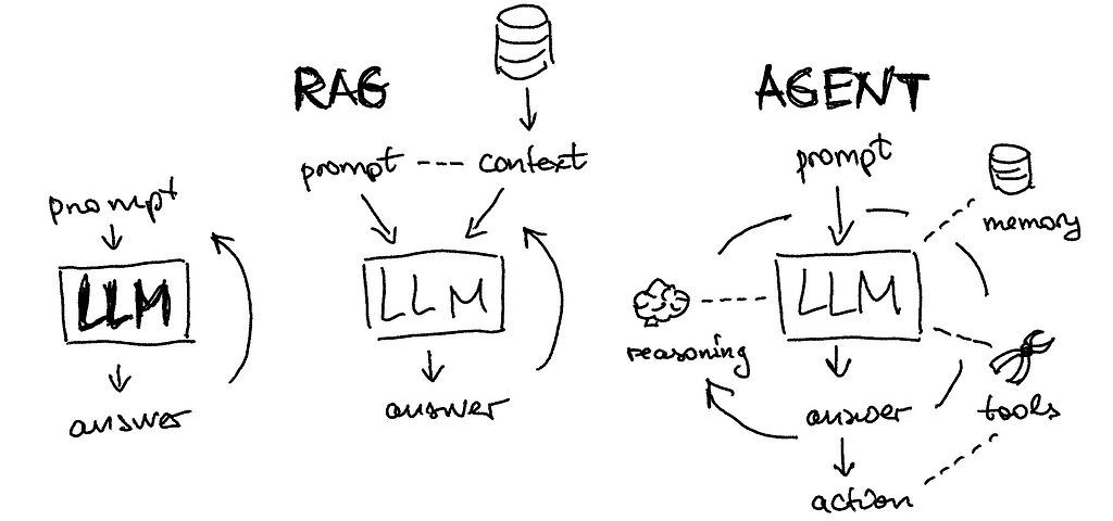
Illustration by author. LLMs are often augmented with external memory via RAG architecture. Agents extend this concept to memory, reasoning, tools, answers, and actions
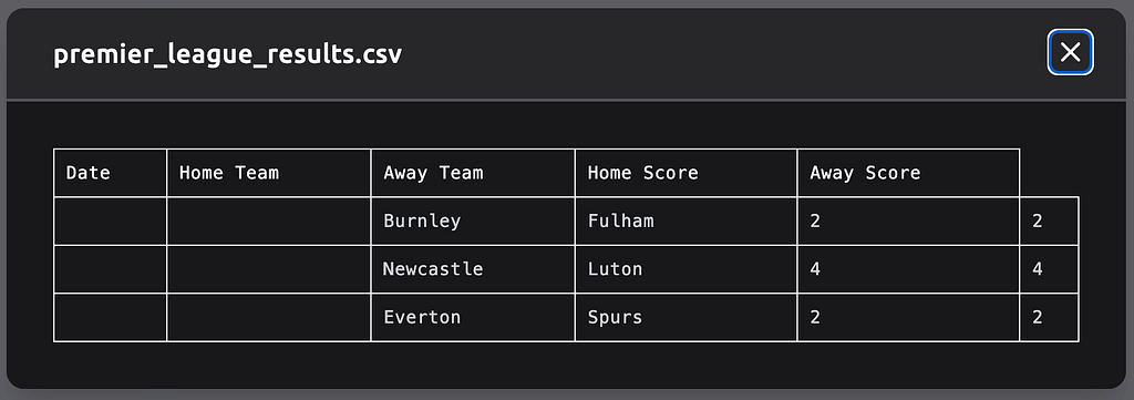
Let’s begin the lecture by exploring various examples of LLM agents. While the topic is widely discussed, few are actively utilizing agents; often, what we perceive as agents are simply large language models. Let’s consider such a simple task as searching for football game results and saving them as a CSV file. We can compare several available tools:
GPT-4 with search and plugins: as you will find in the chat history here, GPT-4 failed to do the task due to code errors
AutoGPT through https://evo.ninja/ at least could generate some kind of CSV (not ideal though):
Since the available tools are not great, let’s learn from the first principles of how to build agents from scratch. I am using amazing Lilian’s blog article as a structure reference but adding more examples on my own.
Step 1: Planning
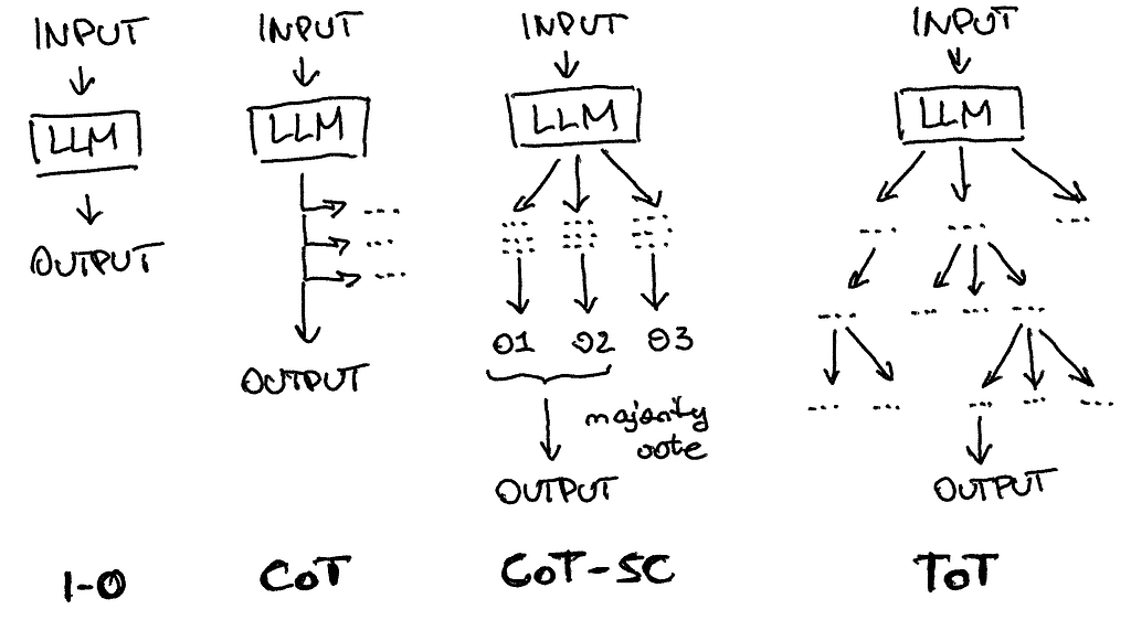
The visual difference between simple “input-output” LLM usage and such techniques as a chain of thought, a chain of thought with self-consistency, a tree of thought
You might have come across various techniques aimed at improving the performance of large language models, such as offering tips or even jokingly threatening them. One popular technique is called “chain of thought,” where the model is asked to think step by step, enabling self-correction. This approach has evolved into more advanced versions like the “chain of thought with self-consistency” and the generalized “tree of thoughts,” where multiple thoughts are created, re-evaluated, and consolidated to provide an output.
In this tutorial, I am using heavily Langsmith, a platform for productionizing LLM applications. For example, while building the tree of thoughts prompts, I save my sub-prompts in the prompts repository and load them:
from langchain import hub from langchain.chains import SequentialChain
You can see in this notebook the result of such reasoning, the point I want to make here is the right process for defining your reasoning steps and versioning them in such an LLMOps system like Langsmith. Also, you can see other examples of popular reasoning techniques in public repositories like ReAct or Self-ask with search:
Reflexion (Shinn & Labash 2023) is a framework to equip agents with dynamic memory and self-reflection capabilities to improve reasoning skills.
Chain of Hindsight (CoH; Liu et al. 2023) encourages the model to improve on its own outputs by explicitly presenting it with a sequence of past outputs, each annotated with feedback.
Step 2: Memory
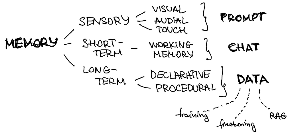
We can map different types of memories in our brain to the components of the LLM agents’ architecture
Sensory Memory: This component of memory captures immediate sensory inputs, like what we see, hear or feel. In the context of prompt engineering and AI models, a prompt serves as a transient input, similar to a momentary touch or sensation. It’s the initial stimulus that triggers the model’s processing.
Short-Term Memory: Short-term memory holds information temporarily, typically related to the ongoing task or conversation. In prompt engineering, this equates to retaining the recent chat history. This memory enables the agent to maintain context and coherence throughout the interaction, ensuring that responses align with the current dialogue. In code, you typically add it as conversation history:
from langchain_community.chat_message_histories import ChatMessageHistory from langchain_core.runnables.history import RunnableWithMessageHistory from langchain.agents import AgentExecutor from langchain.agents import create_openai_functions_agent
Long-Term Memory: Long-term memory stores both factual knowledge and procedural instructions. In AI models, this is represented by the data used for training and fine-tuning. Additionally, long-term memory supports the operation of RAG frameworks, allowing agents to access and integrate learned information into their responses. It’s like the comprehensive knowledge repository that agents draw upon to generate informed and relevant outputs. In code, you typically add it as a vectorized database:
from langchain.text_splitter import RecursiveCharacterTextSplitter from langchain_community.document_loaders import WebBaseLoader from langchain_community.vectorstores import FAISS from langchain_openai import OpenAIEmbeddings
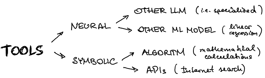
In practice, you want to augment your agent with a separate line of reasoning (which can be another LLM, i.e. domain-specific or another ML model for image classification) or with something more rule-based or API-based
ChatGPT Plugins and OpenAI APIfunction calling are good examples of LLMs augmented with tool use capability working in practice.
Built-in Langchain tools: Langchain has a pleiad of built-in tools ranging from internet search and Arxiv toolkit to Zapier and Yahoo Finance. For this simple tutorial, we will experiment with the internet search provided by Tavily:
from langchain.utilities.tavily_search import TavilySearchAPIWrapper from langchain.tools.tavily_search import TavilySearchResults
Custom tools: it’s also very easy to define your own tools. Let’s dissect the simple example of a tool that calculates the length of the string. You need to use the @tooldecorator to make Langchain know about it. Then, don’t forget about the type of input and the output. But the most important part will be the function comment between “”” “”” — this is how your agent will know what this tool does and will compare this description to descriptions of the other tools:
from langchain.pydantic_v1 import BaseModel, Field from langchain.tools import BaseTool, StructuredTool, tool
@tool def calculate_length_tool(a: str) -> int: """The function calculates the length of the input string.""" return len(a)
You can find examples of how it works in this script, but you also can see an error — it doesn’t pull the correct description of the Neurons Lab company and despite calling the right custom function of length calculation, the final result is wrong. Let’s try to fix it!
Step 4: All together
I am providing a clean version of combining all the pieces of architecture together in this script. Notice, how we can easily decompose and define separately:
All kinds of tools (search, custom tools, etc)
All kinds of memories (sensory as a prompt, short-term as runnable message history, and as a sketchpad within the prompt, and long-term as a retrieval from the vector database)
Any kind of planning strategy (as a part of a prompt pulled from the LLMOps system)
The final definition of the agent will look as simple as this:
As you can see in the outputs of the script (or you can run it yourself), it solves the issue in the previous part related to tools. What changed? We defined a complete architecture, where short-term memory plays a crucial role. Our agent obtained message history and a sketchpad as a part of the reasoning structure which allowed it to pull the correct website description and calculate its length.
Outro
I hope this walkthrough through the core elements of the LLM agent architecture will help you design functional bots for the cognitive tasks you aim to automate. To complete, I would like to emphasize again the importance of having all elements of the agent in place. As we can see, missing short-term memory or having an incomplete description of a tool can mess with the agent’s reasoning and provide incorrect answers even for very simple tasks like summary generation and its length calculation. Good luck with your AI projects and don’t hesitate to reach out if you need help at your company!
We use cookies on our website to give you the most relevant experience by remembering your preferences and repeat visits. By clicking “Accept”, you consent to the use of ALL the cookies.
This website uses cookies to improve your experience while you navigate through the website. Out of these, the cookies that are categorized as necessary are stored on your browser as they are essential for the working of basic functionalities of the website. We also use third-party cookies that help us analyze and understand how you use this website. These cookies will be stored in your browser only with your consent. You also have the option to opt-out of these cookies. But opting out of some of these cookies may affect your browsing experience.
Necessary cookies are absolutely essential for the website to function properly. These cookies ensure basic functionalities and security features of the website, anonymously.
Cookie
Duration
Description
cookielawinfo-checkbox-analytics
11 months
This cookie is set by GDPR Cookie Consent plugin. The cookie is used to store the user consent for the cookies in the category "Analytics".
cookielawinfo-checkbox-functional
11 months
The cookie is set by GDPR cookie consent to record the user consent for the cookies in the category "Functional".
cookielawinfo-checkbox-necessary
11 months
This cookie is set by GDPR Cookie Consent plugin. The cookies is used to store the user consent for the cookies in the category "Necessary".
cookielawinfo-checkbox-others
11 months
This cookie is set by GDPR Cookie Consent plugin. The cookie is used to store the user consent for the cookies in the category "Other.
cookielawinfo-checkbox-performance
11 months
This cookie is set by GDPR Cookie Consent plugin. The cookie is used to store the user consent for the cookies in the category "Performance".
viewed_cookie_policy
11 months
The cookie is set by the GDPR Cookie Consent plugin and is used to store whether or not user has consented to the use of cookies. It does not store any personal data.
Functional cookies help to perform certain functionalities like sharing the content of the website on social media platforms, collect feedbacks, and other third-party features.
Performance cookies are used to understand and analyze the key performance indexes of the website which helps in delivering a better user experience for the visitors.
Analytical cookies are used to understand how visitors interact with the website. These cookies help provide information on metrics the number of visitors, bounce rate, traffic source, etc.
Advertisement cookies are used to provide visitors with relevant ads and marketing campaigns. These cookies track visitors across websites and collect information to provide customized ads.