Mistral AI’s open-source Mixtral 8x7B model made a lot of waves — here’s what’s under the hood
Originally appeared here:
Demystifying Mixtral of Experts

Mistral AI’s open-source Mixtral 8x7B model made a lot of waves — here’s what’s under the hood
Originally appeared here:
Demystifying Mixtral of Experts
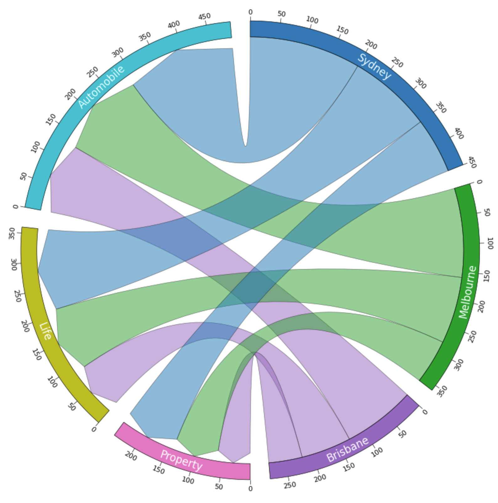

How to draw a fancy chord chart with links using PyCirclize
Originally appeared here:
Probably the Best Data Visualisation for Showing Many-to-Many Proportion In Python
A method to balance multiple objectives for your recommendation output
Originally appeared here:
How to Optimize Recommendation Results with Genetic Algorithm
Go Here to Read this Fast! How to Optimize Recommendation Results with Genetic Algorithm


My tips and experience to become a high quality data scientist
Originally appeared here:
How To Advance In Data Science

I recently decided it was time to make a change in my life. I have been working since I was 14 years old (tell me you are from Gen X without telling me you are from Gen X) and in all of these decades I have always worked for someone else. I very much remember the dot com bust in the early 2000’s when there were plenty of tech layoffs, but it felt mild relative to what is going on today. Perceiving that company loyalty is a thing of the past along with the desire to be my own boss, I decided that it was time to start my own company to do data science and freelancing. What I have discovered in the past 3 months of doing so is that going solo is very viable, even during times of layoffs, with proper planning. So I wanted to write about my experience getting started in the hopes that it can help some others out there who might be having a hard time finding the next thing. This is written from a US perspective, so there are some mechanics that will likely be different in other countries, but the general ideas remain the same.
Before I begin, I want to give a shout out to Brett Trainor, who created an online group called “The Corporate Escapee.” Early in my journey I came across him on TikTok and his videos and other content of his I found really gave me the motivation and courage to take the leap. Check him out!
Let’s face it. Many (most?) of us are raised with the idea that working for a company means job security. So many (most?) of us, when we move between jobs, are moving between companies rather than opportunities. There can be great stability in working for a company. You are guaranteed certain benefits like a paycheck of a known amount provided at regular intervals. You get other things too like health insurance, career guidance and management, training opportunities, retirement savings, etc. In going out on your own, none of those things are guaranteed. So it is no wonder that many (most?) people think of companies as being the most stable and reliable places to work.
This is also rooted in history. For a significant portion of the 20th century retirement was based on a pension and your pension was based on how many years you worked for a company and your salary during that time. The idea was that you were guaranteed income from the company after your retirement. In some cases your pension could even be passed down to your children. It was a great deal! But like the dot com collapse in the early 2000’s, many pension programs were dissolved due to bankruptcy, mismanagement of funds, or other catastrophic investment losses, leading to the loss of retirement by hard working employees. The rise of the 401k retirement system was upon us. That system resulted in a retirement income that was portable, meaning you didn’t have to work your entire career for the same employer to have decent retirement savings. Hence, workers no longer have to rely on a company benefit (pension) to be able to retire.
Going out on your own means that you no longer have the security of these things (salary, 401k contributions, health insurance, etc.). It is natural to be fearful of this. However, in this time of layoffs that rival the early 2000’s, I ask whether that feeling of security working for a company is just a myth?
Also, consider what the job market is like right now. From both my direct experience as well as through conversations within my network I know that open roles for data scientists are presently resulting in thousands of applicants. If you are applying for these roles, the odds of getting a call back are very, very slim. You are literally one of thousands of people they are considering. However, if you go out solo, you will be talking directly to the person making the decisions on contracting. Further, unlike many companies that post open roles and then never hire people into them, if they are talking to you at all it likely is because they have real work that needs to be done. If they are even talking to someone else, it is likely that there are only a small handful of potential applicants. Your odds of getting noticed are much better once you can make contact. For more on how to do this, see my section on networking below.

I have discovered there are many, many benefits of working as a freelancer. As I started writing this section, I realized that it was not possible for me to come up with a ranked list, so this is just my attempt at getting some of them written down.
It really comes down to this: I get to pick what I work on, when I work on it, and for whom I am working. Let’s address these in order.
As my career has evolved, I have developed a deep interest in both natural language processing (NLP) and graphs. It turns out that this is a great combination for working with large language models (LLMs) and generative AI. In my previous roles if I wanted to work on these things I would have needed management permission based on business need for the work to be approved. Now I can specifically seek out work in those areas.
One of the great things about being your own boss is that you make the rules. So if you decide that you are only going to work 4 days per week (or even less!), great. If you don’t want to be sitting at your desk from 9–5, don’t! You have infinite freedom here to define what your work life is like and you can optimize it however you want! In my case, I love to ski and live 5 miles from a world-class ski resort. So I make the rules where I can decide to go out and ski whenever I like — and my boss fully supports that!
As for picking who you work for, what I mean by this is that you are free to take on work for whomever you choose, not just because some manager has directed you to do so.
I have to tell you that in the process of going solo, these freedoms have really been what has been most striking! While I knew in theory that they existed, when you actually start living and working this way you can come to a much better realization of work-life balance. For the first time in my working career I feel like I actually have control over my work and my happiness. I am not subjected to the whims of an employer who may or may not have loyalty to me. And let’s face it, corporate loyalty is a thing of the past.
In the next section we will look at getting started and hopefully some of these benefits become clear.

There are two key things that will help you be successful if you decide to try this out: planning (financial and business) and networking.
There is a lot that should go into this before you strike out on your own. Much of it is financial. You need to know that you will likely be without a paycheck for a bit and it might take you a few months or more to build back to your full, corporate paycheck. So if you have the opportunity to save some money to get you through that time, it will really help.
Second, you should sit down and do the math looking at how much money you need to bring in per month since this will be important in determining your rates. In my case, my goal was to replace my corporate salary. I am the primary breadwinner (and sometimes sole breadwinner since my spouse works a seasonal job) for my family. So I looked at not only my salary, but also the cost of health insurance, how much money I was putting into my retirement savings, and my expected expenses for running the business (to include paying for lawyers and accountants). This determined what my gross income needed to be. Next, you have to know that when you are self employed in the US you will be paying quarterly estimates on your income taxes. This amounts to approximately 35%. Using this I was able to determine what my net income per month needs to be in order to break even on my corporate salary.
Next, you need to consider what your pricing model will be. Will you be charging hourly and then tracking your hours? Will you be on retainer for a fixed fee per month? Maybe you will charge on a per project basis? As you looking to be the person doing the coding (freelance) or advising on how to get a project going (consulting)? Maybe instead you are seeking a fractional role? Getting started, I found it easiest to wrap my head around the hourly freelance concept. People who have been working solo for a while will tell you that this is not ideal and that it is much more desirable to be on retainer. At this stage, my clients prefer hourly billing, so that is what I am doing. So it is easy to see that you can take that break-even monthly net income and work backwards to what hourly rate you should be charging to get there.
But here is a gotcha! I originally thought I would take that amount and assume 40 hours per week to work out the hourly rate. Wrong! You need to build in some slack because, as it turns out, most of us don’t actually work 40 hours per week, even in corporate. For example, I do not charge clients when I have lunch, walk the dog, work out, or pick my kid up from school. I also only bill when I am at my keyboard working on things for my clients and not when I happen to be “sitting around” just thinking about their problems. You also need to allocate time for networking, setting up the next contracts, etc. A mentor told me that a good rule-of-thumb was to assume that you will actually only be billing 60% of the time. This gives you a practical buffer such that you are still hitting your goal net income on a realistic number of billable hours.
So based on this, I set my hourly rate. When I compared that rate to contractors of similar experience levels I had worked with in previous roles, it seemed realistic. (Consider that contracting shops will typically tack on around a third for their fees, so the rate a contractor actually takes home is typically around two thirds of what the contract shop bills for.) I utilized my network and bounced this rate off of them and they all agreed that my hourly rate was appropriate.
In addition to having planned for the finances of the situation, you should also plan out the setup for the business. There are many different ways you can do this and I am not a lawyer so you should consult with one before making your decision. One way you can do this is just to be working as an individual, independent contractor (sometimes referred to as a 1099 based on the tax documentation used in this approach). Another option is to set up an actual business such as an LLC or Corporation. I elected to create an LLC because it provides a certain amount of legal protection and separation between the business’s finances and my personal finances (i.e. it is hard for clients to go after your personal finances if they sue the business). I enlisted the aid of a lawyer to help me set one up in my home state. There are also plenty of online options for doing this where you might be able to do it yourself, but I felt the peace of mind of having a trained professional do this for me was worth it.
I also worked with my accountant who does my family’s personal taxes to help with the business taxes. I cannot say too much about this since I have not submitted my first quarterly estimated payment yet, so that will likely be included in a future post. However, one thing that I can say at this stage is that it is VERY important that you save receipts for EVERYTHING. There are many expenses you will have such as fees paid to the lawyer, computers, web pages and domain names, etc. that are tax deductible. However, they have to be tracked and accounted for. You will save yourself a lot of time later if you start by religiously tracking these things.
Finally, once you have the business set up, it can help setting up a separate bank account for it. While maybe not required, I find this helpful since it really keeps the business finances cleanly separated from my personal finances. When it is time to get paid, the business cuts you a check. Having a debit card linked to that account further helps keep things separate.
We have all been told, practically since infancy, that networking is important. That is especially true when freelancing or consulting. When I decided that I would start my own business and particularly once the LLC was formed, the first thing I did was to reach out to my network to let them know what I was doing. I have been very fortunate in my career, about 23 years to this point, to have met many great people working directly in data science or in companies who regularly work with data scientists. I initially started by quietly talking with a few of my mentors, but then when I was ready I announced on LinkedIn that I had launched the company. I was very fortunate that there were some people in my network who had need for someone to do freelancing LLM work on an hourly basis. Some of the interest came from people I had worked with in the past. Other interest came from people who had seen content of mine online.
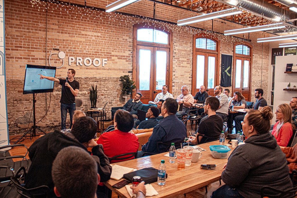
In my opinion, networking is the area where people who have been laid off (or other considering this as an option for layoff protection) might have a more difficult time than financial planning. However, that doesn’t mean that you can’t build your network quickly. Attending (better yet: speaking at) conferences and meetups is a great way to do this. Ideally, you have an employer that is willing to pay for you to go. Even if they aren’t, consider this an investment in yourself and your career. If you are running a solo business already, you can write these trips off. Many of the bigger conferences offer discounts to people who are unemployed. Additionally, most (many? all?) conferences need volunteers to help at them. So even if you are not speaking, you can still have the opportunity to meet and network with people. Writing blog posts and participating in open source projects are also ways to grow your network. Additionally, it can be helpful to have a portfolio of work for others to view.

While I am still new to freelancing, I have learned some things that have helped me in the first few months be more efficient. Pretty much all of them have to do with the philosophy of making it easy for your clients.
You should consider that there are some tools (which are business expenses) that will be expected. First, just like working in corporate you should have an email address specific to your work. For me, I bought a domain name for my business and set up a Google workspace for that domain. This will also help when certain platforms ask for your work email address and scoff at a Gmail address. I then take advantage of Google Sheets for managing my expenses and time tracking. (I might move this to QuickBooks, but haven’t made that transition yet. Ask me after this first round of taxes if it is worth it.)
Next, I found it very helpful to have a means to allow people to easily book time with me. I found Calendly to be a great option for this. If you are going to do this, I would suggest that you place some limits on the hours that people can book with you. Remember that when you are not billing, you are not earning. So try to avoid spending all of your time in prospecting meetings.
I also have put some thought into how to send invoices and receive payment. Again, the idea here is to make it easy for your client to pay you. You can set up accounts with Stripe or Square to do this or QuickBooks can do it for you. However, bear in mind that they will charge fees of something like 3% on the total invoice. This can really add up. Another option for receiving payment is directly via bank transfer/ACH, which can be harder for your clients but does not take off those fees. Be prepared to work with your clients on what works best for them. And bear in mind that having a business banking account, whether for ACH transfer or Stripe/Square/QuickBooks, means that you are not handing out your personal banking information to clients.
Finally, it is important to know that every client will have a different set of tools that they are most comfortable with. Some prefer Slack. Others are very Microsoft-centric, preferring Teams. While I personally have very strong personal preferences, I have found it important to be able to work within any of them. In my case, this means that I had to buy a PC since my Linux machine doesn’t handle Teams very well. C’est la vie.

It is true that I have only been working solo for a few months now. So it is too early for me to say if I have been 100% successful. However, I am incredibly fortunate in that I have thus far achieved all of the goals I have had for my company at this point. And I am greatly enjoying the new found freedom, flexibility, and balance in my life.
While I began this post with a discussion on the fact that many people do not consider freelancing because of the lack of security, I actually find myself feeling much more secure than in the corporate world. For one, I am not subjected to layoffs. In fact, my guess is that more companies will start turning to freelancers, contract employees, and fractional employees because of their layoffs. It is not like they have decreased the amount of work that has to be done just because they have laid people off. They will need people to come in and do that work, even if they are not adding to their head count. Contracts will come and go and constantly securing contracts is part of this lifestyle.
All of that being said, I view my true definition of success as being whether I can sustain this work — and my goal of replacing my corporate salary through my solo endeavors — beyond just my first few contracts. We will not truly know the answer to that for some time. But right now things are looking positive!!!

What I Learned in my First 3 Months as a Freelance Data Scientist was originally published in Towards Data Science on Medium, where people are continuing the conversation by highlighting and responding to this story.
Originally appeared here:
What I Learned in my First 3 Months as a Freelance Data Scientist
Go Here to Read this Fast! What I Learned in my First 3 Months as a Freelance Data Scientist

tl;dr version: A team of students helped design and carry out an experiment to determine whether bowls of Lucky Charms are equally “lucky” over the course of a box of cereal. Turns out, not so much. We estimate a decrease of approximately 2.7 total charms per additional bowl on average. This corresponds to more than a 50% drop-off in charms from the first bowl to the last. The weight of cereal also appears to play a role, and for each 1g of cereal we estimate approximately 0.5 more charms on average with bowl held constant. The interaction between bowl and weight is not statistically significant.
See this GitHub repository for the data, code, photos, etc.
In the early 2010’s there was a kerfuffle on the Internet over an investigation into whether or not “Double Stuf” Oreos were actually double-stuffed. (They’re not.) It was an engaging idea, and a substantial amount of material has been written about it since, see here for starters. The discussion caused enough splash that some teachers were evidently repeating the experiment as an activity in their classrooms, and local students have reported performing similar experiments at their own schools more than 10 years later.
One morning in the summer of 2023 I was eating a bowl of Lucky Charms for breakfast. The box was nearly empty and I sighed to myself, “Can’t wait until this box is done so I can open up a new one…” Now, if you’re anything like me, or millions of other people, then you love Lucky Charms, and you’ve loved them for as long as you can remember, being around for 60 years and all. They truly are Magically Delicious. But sitting there on that summer morning of discontent with a spoon in my hand it struck me that the bowl of cereal I was eating just didn’t quite seem as magical as the earlier bowls had been. It was missing something. (The charms, of course.) Was it my imagination? Could this effect be real? And if so, could it be measured?
I happened to be teaching an undergraduate probability & statistics course at the time and the four students and I were determined to find out.
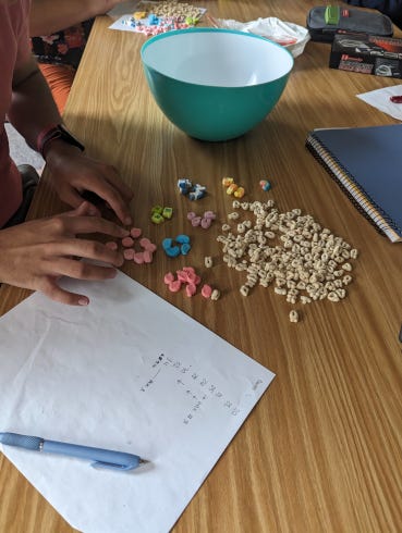
After some discussion, the team decided on the following materials and methods.
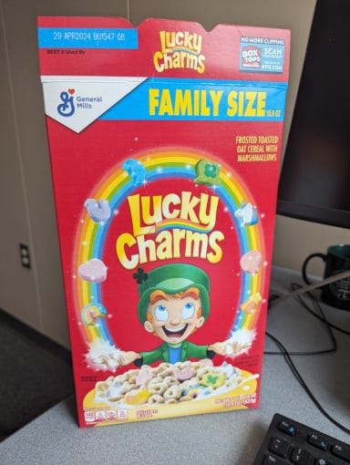
The Lucky Charms were purchased from our local retailer—Wal-Mart. There was nothing special about n = 6 boxes, it was simply the number of boxes a person could carry with two hands to the 6th floor of Cafaro Hall in a single trip. The kitchen scale was for measuring the weight of cereal, which the team thought might be important, and the scale would also help with data collection because we didn’t want to be overly preoccupied with sampling the exact same amount of cereal every time.
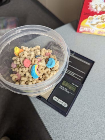
For the purposes of this experiment, a “bowl” was taken to be approximately 1 serving of cereal as recommended by the box (1 cup or 36g), even though it is ridiculous for anybody but a tiny magic leprechaun to get by on 36g of Lucky Charms for breakfast. The team was not especially picky about maintaining bowl size consistency, anything close to 1 cup was considered good enough. We were accounting for mass of cereal with the kitchen scale anyway and were shooting for a healthy range of observed weights.

Each bowl of cereal was poured directly from the box into the plastic container, weighed, and then emptied onto the table surface for counting. The toasted oats were separated from the marshmallows and discarded. Next the following eight (8) charm types were recognized and their number recorded: Pink Hearts, Rainbows, Purple Horseshoes, Blue Moons, Green Clovers, Unicorns, Tasty Red Balloons, and Orange Stars.
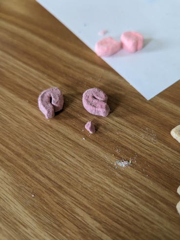
Occasionally there were little marshmallow bits in the bowl; not every charm was 100% intact. To deal with this, the team attempted to classify the bit into the type of charm (Green Clover, Blue Moon, etc.), and if the type could be determined, then that bit was counted as 1 in the respective category. If the bit was nondescript or too small for type identification then it was discarded.
Data were collected during two separate class meetings. The students worked in pairs to pour and count the charms. I helped with the scale and recording a hard copy of weight values as they were called out for entry into the computer. The team got into a data collection groove and by the end of the experiment all 4 students were pouring and counting charms independently.
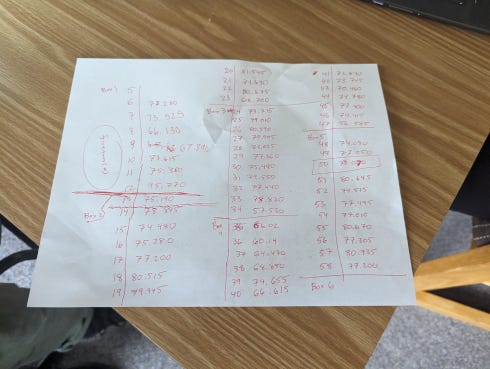
The plastic container + cereal were weighed together each round, and the weight of the container (measured at the start of the experiment) was subtracted from the observed total weight. The charms were entered into their respective columns and totaled.
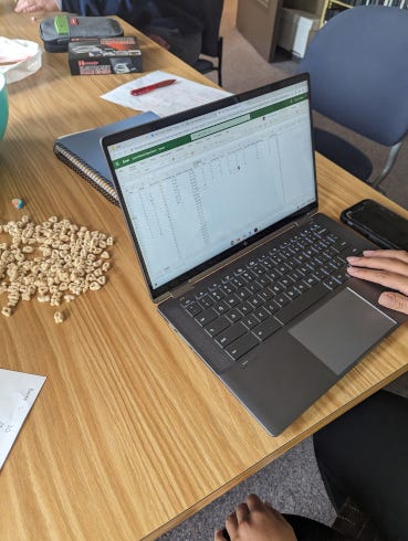
Here is some R code to read in and show the top of the dataset (first 6 rows). The data and all code are shared in this GitHub repository.
library(readxl)
Lucky <- read_excel("Lucky.xlsx")
Lucky$Box <- as.factor(Lucky$Box)
head(Lucky)
Equipped with these data we can report things like the mean observed Weight was approximately 46.3g, the maximum number of a particular charm in any one bowl was 15 (Pink Hearts tied with Purple Horseshoes), and so forth. Indeed, we could spend all day computing statistics on this dataset to our Pink Heart’s content, but at the moment we are primarily focused on Totcharms and how it relates to Bowl and maybe Weight to a lesser extent.
Here is a graph of Totcharms by Bowl, colored by Box:
Lucky |> ggplot(aes(x = Bowl, y = Totcharms, color = Box)) +
  geom_point(size = 3) +
  labs(y = '# Charms') -> p1
p1
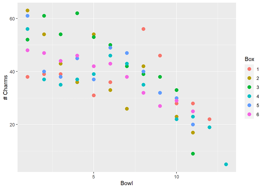
Here we see a clear decreasing trend in Totcharms as Bowl increases, and the pattern is surprisingly linear. There may be a slight curvature. The colors are tricky to pick out, so let’s make a line plot and highlight a couple of series:
sizes <- c(2, 1, 2, 1, 1, 1)
alphas <- c(1, 0.2, 1, 0.2, 0.2, 0.2)
Lucky |> ggplot(aes(x = Bowl, y = Totcharms)) +
  geom_line(aes(colour = Box, linewidth = Box, alpha = Box)) +
  scale_discrete_manual("linewidth", values = sizes) +
  scale_alpha_manual(values = alphas, guide = "none")

There is a general trend downward for all series, but the path to get there varies for individual boxes. Notice how Box 3 starts high and stays high for a few bowls before dropping off smoothly to Bowl 10, crashing promptly afterwards. Look at how Box 1 starts the lowest of the crowd, increases after Bowl 5, peaks at Bowl 8, then nosedives down to Bowl 12. The data would suggest that charms were more concentrated near the top of Box 3, but were more clustered in a pocket near the middle of Box 1. Some boxes bounce around, other boxes drift in more of a straight line downward. Put it all together, though, and the overall trend is decreasing and linear. Note that every box made it at least to Bow1 = 11, but only two boxes had 12 bowls, and a single box (Box 4) lasted to Bow1 = 13.
Now let’s take a look at Totcharms versus Weight:
Lucky |> ggplot(aes(x = Weight, y = Totcharms, color = Box)) +
  geom_point(size = 3) +
  labs(x = 'Weight (g)', y = '# Charms') -> p2
p2

This plot is noisy as we might have guessed. We have a nice range of weights, from a minimum under 30g to a maximum near 70g. Notice there was one bowl that clocked-in extraordinarily heavy. The outlier doesn’t have any obvious explanation, but if we dig a little deeper and plot Weight versus Bowl we may gain some insight:
Lucky |> ggplot(aes(x = Bowl, y = Weight, color = Box)) +
  geom_point(size = 3) + ylim(5, 75) +
  labs(y = 'Weight (g)') -> p3
p3

We see that the extra-heavy bowl was the last Bowl = 12 of Box = 1. The origin of that particular data point has unfortunately been lost to the sands of time, but bearing in mind that it was the first box the team had ever finished, near the end it may have been difficult to judge how much cereal was left, and perhaps all the remainder was dumped into that final bowl—I do the same thing at breakfast all the time when I get close to the end of a box of cereal. If that 12th bowl of 70g had been split into (say) two bowls of 40g and 30g, respectively, then there would have been two boxes that made it all the way to 13 bowls instead of just one, and maybe the models below would have fit the data slightly better. Alas! We will never know. Such is the scientific enterprise.
While there isn’t much of a linear association between Totcharms and Weight by themselves, there is a hidden relationship between Totcharms, Bowl, and Weight which can best be explored with a 3D visualization:
library(plotly)
fig <- plot_ly(Lucky, x = ~Bowl, y = ~Weight, z = ~Totcharms, color = ~Box) |>
  add_markers() |>
  layout(scene = list(xaxis = list(title = 'Bowl'),
                                   yaxis = list(title = 'Weight (g)'),
                                   zaxis = list(title = '# Charms')),
                      legend=list(title=list(text='Box')))
fig
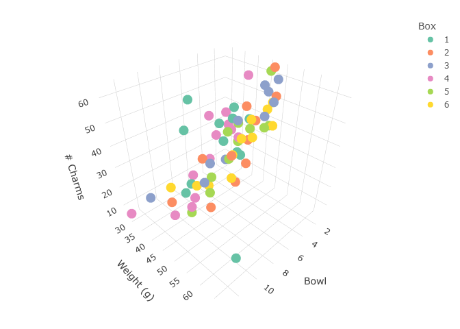
Plots in 3D are super-cool, but the above static display doesn’t do the data justice. I’ve set up an interactive version of the plot at the following link which should work in most mobile/desktop browsers:
Interactive Lucky 3D Scatterplot
Please go there, spin the data around, zoom, pan—check it out. If you spin it around just right you will see that the dots scatter loosely about a flat plane in 3D-space. This is exactly the kind of relationship we are looking for in a multiple linear regression model (we’ll get to that in a minute).
Now let’s try to quantify the linear relationship between these variables. We will start with a simple linear regression model relating Totcharms to Bowl.
Here is the model:
mod1 <- lm(Totcharms ~ Bowl, data = Lucky)
summary(mod1)
##
## Call:
## lm(formula = Totcharms ~ Bowl, data = Lucky)
##
## Residuals:
##      Min       1Q   Median       3Q      Max
## -16.7629  -5.7629  -0.4327   6.2277  22.2277
##
## Coefficients:
##             Estimate Std. Error t value Pr(>|t|)
## (Intercept)  55.1309     2.1237  25.960  < 2e-16 ***
## Bowl         -2.6698     0.2985  -8.945 4.81e-13 ***
## ---
## Signif. codes:  0 '***' 0.001 '**' 0.01 '*' 0.05 '.' 0.1 ' ' 1
##
## Residual standard error: 8.313 on 67 degrees of freedom
## Multiple R-squared:  0.5442, Adjusted R-squared:  0.5374
## F-statistic: 80.01 on 1 and 67 DF,  p-value: 4.807e-13
We see that Bowl is strongly linearly associated with Totcharms. The slope on Bowl is approximately −2.7, in other words, for each additional bowl of Lucky Charms eaten we estimate the average Totcharms to decrease by 2.7 charms. Our coefficient of determination is R² = 0.5442, that is, approximately 54% of the variance in Totcharms is explained by the regression model with Bowl as a predictor. Next we really ought to include a proper residual analysis but we are going to skip it. Suffice it to say that the residual plots are relatively well-behaved. Let’s check out a fitted line plot with confidence bands for the regression line (the default):
p1 + geom_smooth(method = "lm", aes(group=1), colour="black")
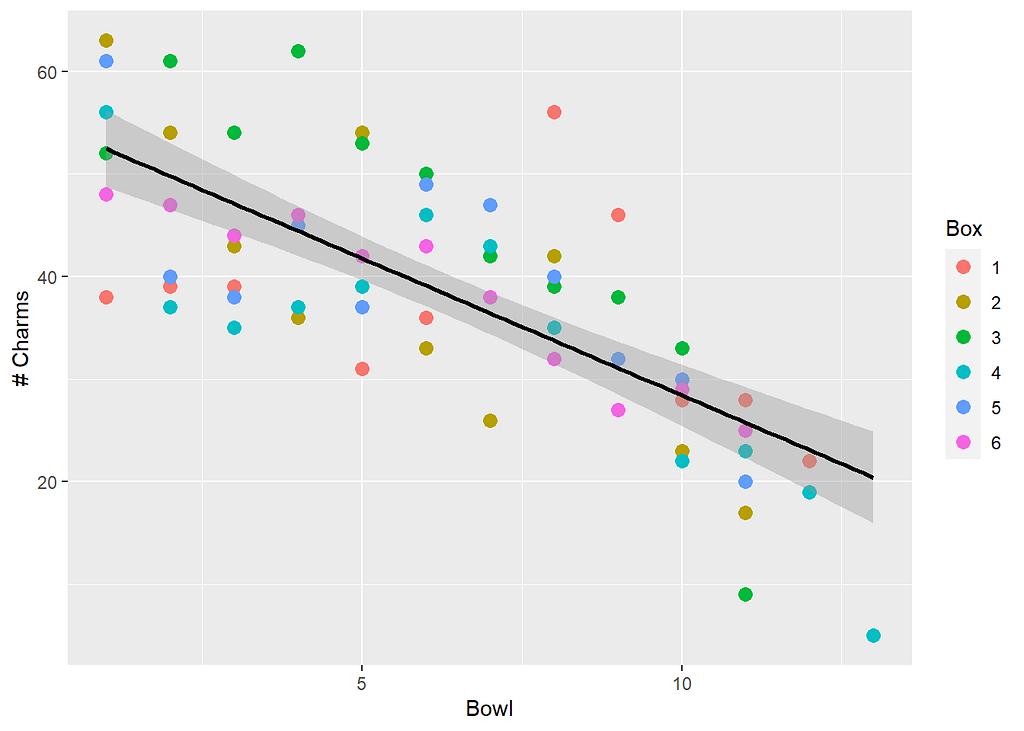
That’s a nice relationship with a clear decreasing trend.
We will do the same thing for Weight, ignoring Bowl for the time being. Here we go:
mod2 <- lm(Totcharms ~ Weight, data = Lucky)
summary(mod2)
##
## Call:
## lm(formula = Totcharms ~ Weight, data = Lucky)
##
## Residuals:
##      Min       1Q   Median       3Q      Max
## -27.0151  -8.7745   0.6901   7.8328  24.4701
##
## Coefficients:
##             Estimate Std. Error t value Pr(>|t|)
## (Intercept)  22.1370    10.5650   2.095   0.0399 *
## Weight        0.3502     0.2256   1.552   0.1254
## ---
## Signif. codes:  0 '***' 0.001 '**' 0.01 '*' 0.05 '.' 0.1 ' ' 1
##
## Residual standard error: 12.1 on 67 degrees of freedom
## Multiple R-squared:  0.0347, Adjusted R-squared:  0.02029
## F-statistic: 2.409 on 1 and 67 DF,  p-value: 0.1254
We do not find Weight to be a very useful predictor of Totcharms on its own, which jives with the scatterplot we saw earlier. We note for reference that the slope on Weight is estimated at 0.3502, that is, each additional 1g of Lucky Charms corresponds to an average Totcharms increase of 0.35 charms. This sounds reasonable: more cereal, more charms. The coefficient of determination is pretty bad: R² = 0.0347, in other words, approximately NONE% of the variance in Totcharms is explained by the regression model with Weight as a predictor. That’s okay; Weight was more of a supplementary device to help control for variability in the cereal amounts. The residual analysis here turns out to be not as bad as it could have been, which is comforting, and we should expect a few problems anyway given the extreme observations on the high/low ends of the weight scale. For the sake of completeness we include another fitted line plot:
p2 + geom_smooth(method = "lm", aes(group=1), colour="black")

I originally planned to use the ggpubr package to put these fitted-line plots together and try to save some space in the discussion, but the plots were cramped and not very informative. Anyway, this is what I was going to do:
library(ggpubr)
ggarrange(p1 + geom_smooth(method = "lm", aes(group=1), colour="black"),
          p2 + geom_smooth(method = "lm", aes(group=1), colour="black"),
          align = 'h', labels=c('A', 'B'), legend = "right",
          common.legend = TRUE)
Now for the fun part: we’ve explored the relationships Totcharms ~ Bowl and Totcharms ~ Weight individually, but what happens if we put them together? Let’s find out:
mod3 <- lm(Totcharms ~ Bowl + Weight, data = Lucky)
summary(mod3)
##
## Call:
## lm(formula = Totcharms ~ Bowl + Weight, data = Lucky)
##
## Residuals:
##      Min       1Q   Median       3Q      Max
## -12.8825  -5.4425  -0.9975   5.2475  26.5304
##
## Coefficients:
##             Estimate Std. Error t value Pr(>|t|)
## (Intercept)  33.3168     6.8655   4.853 7.78e-06 ***
## Bowl         -2.7552     0.2796  -9.855 1.35e-14 ***
## Weight        0.4819     0.1452   3.318  0.00148 **
## ---
## Signif. codes:  0 '***' 0.001 '**' 0.01 '*' 0.05 '.' 0.1 ' ' 1
##
## Residual standard error: 7.754 on 66 degrees of freedom
## Multiple R-squared:  0.6094, Adjusted R-squared:  0.5976
## F-statistic: 51.49 on 2 and 66 DF,  p-value: 3.363e-14
Check it out! Now Bowl and Weight are both strongly linearly associated with Totcharms. The slope on Bowl is almost identical to what it was before, −2.7, but the estimated slope on Weight has now increased to nearly 0.5 charms for each additional 1g of cereal. Our (adjusted) Multiple R² has jumped to almost 60%—this is remarkable considering the small sample size (n = 6), the general noise level of the dataset, and maybe some questionable design choices (every little marshmallow bit counts as 1, etc.). In retrospect, it is kind of amazing that the data didn’t turn out a lot worse. Real data collected by hand in the wild are seldom so good-natured.
The code for this visualization is a bit more involved than the other examples and has been omitted for brevity, but you can check it all out in this GitHub Gist. Let’s get on with the plot:

Again: a super-cool plot but the static version doesn’t do the data justice. Check out the interactive version instead:
Interactive Lucky 3D with Regression Plane
Interactive 3D-plots are a lot of fun. I hope you enjoy playing with the graph as much as I have. As a final remark, in the tl;dr statement we claimed that the interaction between Bowl and Weight is not significant. The reader can confirm it isn’t with the following (output omitted):
summary(lm(Totcharms ~ Bowl * Weight, data = Lucky))
I originally thought that either the whole thing would turn out to be a figment of my imagination or the effect would be too small to detect without LOTS AND LOTS of Lucky Charms. I was wrong on both counts. The effect is real, and it is big enough to detect with a handful of boxes, literally two hands full.
The full model leads us quickly to some startling conclusions. For example, how many charms do we estimate in the first bowl of a box of Lucky Charms? We saw earlier that the average Weight in this study was 46.3g. When Box = 1 the model estimates the average Totcharms to be
33.3168 + (-2.7552)*1 + 0.4819*46.3
## [1] 52.87357
That is, around 53 charms in the first bowl of cereal—Mmm, mouth’s watering already. What about the last bowl? Okay, not every box made it to Bowl 13, but they all made it to Bowl = 11. How many charms?
33.3168 + (-2.7552)*11 + 0.4819*46.3
## [1] 25.32157
WOW. 25.3 charms on average. This corresponds to a 52% reduction in charms from the first bowl to the eleventh. No, it was most definitely not my imagination. Forget multiple linear regression models and fancy 3D plots, a hungry toddler could detect this difference wearing a blindfold.
Next question: Why is there a drop-off? An analysis on physical grounds might go something like this: Consider a box of Lucky Charms to be a simple mechanical mixture of frosted toasted oats and marshmallows. Many external forces agitate the box over the course of its lifetime, such as jostling during transport, placement on the store shelf, and transit to the home, not to mention activity in and around the cupboard. This inevitably leads to a shifting of contents, with the slightly less dense marshmallows migrating toward the top of the box, and the denser toasty oats settling toward the bottom.
This rationale is logical, anyway. But it leaves some related questions unanswered:
These open questions will have to wait for another day.
Since the original experiment in Summer 2023, I’ve rerun the experiment a couple more times with other groups of students. The first was in November 2023 with middle schoolers on YSU MegaMath Day. I failed to give the MegaMath students very specific instructions and before I knew it all teams had removed the plastic bags of cereal from the box and were scooping from the middle of the bag spread flat on the tabletop. I couldn’t blame them; it is easier to scoop cereal from the middle with the bag out in the open. Unfortunately, this approach completely destroys any natural density sort-order that may have have been present, the key underlying element we suspect is at play, which compromises the integrity of the experiment. Plus, I doubt anybody’s parents ever let them eat their Lucky Charms that way.
The second was in February 2024 with high school students at YSU MathFest in a sequence of two workshops. This time I was ready for them. I put together and distributed a data collection sheet (which you can find here) with more detailed guidance. You can check out the extra datasets on GitHub in the extraData directory.
Moving forward, more data are needed to better estimate the Lucky Charm drop-off, and it would be interesting to test strategies for distributing the charms more uniformly throughout the box. If successful, the first bowl of the box might not be so magical, but on the other hand, maybe those final bowls won’t feel like such a chore waiting to open the next brand new box of Lucky Charms!
This experiment and these results would not have been possible without the infectious enthusiasm and tireless attention to detail of all four STAT 3743 students in Summer 2023: Brenna Brocker, Kate Coppola, Gavin Duwe, and Haziq Rabbani. I thank them for hiking down this statistical path with me. I would also like to thank the Department of Mathematics and Statistics at Youngstown State University for supporting both this research and additional data collection at YSU MegaMath Day and YSU MathFest.
In case it isn’t already abundantly clear, the author is a Lucky Charms fan, so too are the 4 students. The outcomes reported here were not and are not meant as a critique of General Mills, Inc., its subsidiaries, their factory production standards, nor the fine humans and robots gainfully employed there. We are all bound by the same Laws of Physics, and that includes boxes of breakfast cereal.
And full disclosure: I’ve taken a peek at the extra data collected in the reruns of the experiment. From what I can tell the effect is still present, but it isn’t as dramatic. I don’t know if this is because the effect is truly smaller than what we originally estimated, or if it is somehow related to the data collection protocol in the middle/high school setting. Only time — and more data — will tell.
In putting together this article I tried to keep a record of the places I went to find code to build the plots that I wanted and below is a mostly complete list, but maybe I missed some links. If you notice something I missed, then please alert me in the comments and I will fix it.
How Lucky is a Bowl of Lucky Charms? was originally published in Towards Data Science on Medium, where people are continuing the conversation by highlighting and responding to this story.
Originally appeared here:
How Lucky is a Bowl of Lucky Charms?
Go Here to Read this Fast! How Lucky is a Bowl of Lucky Charms?
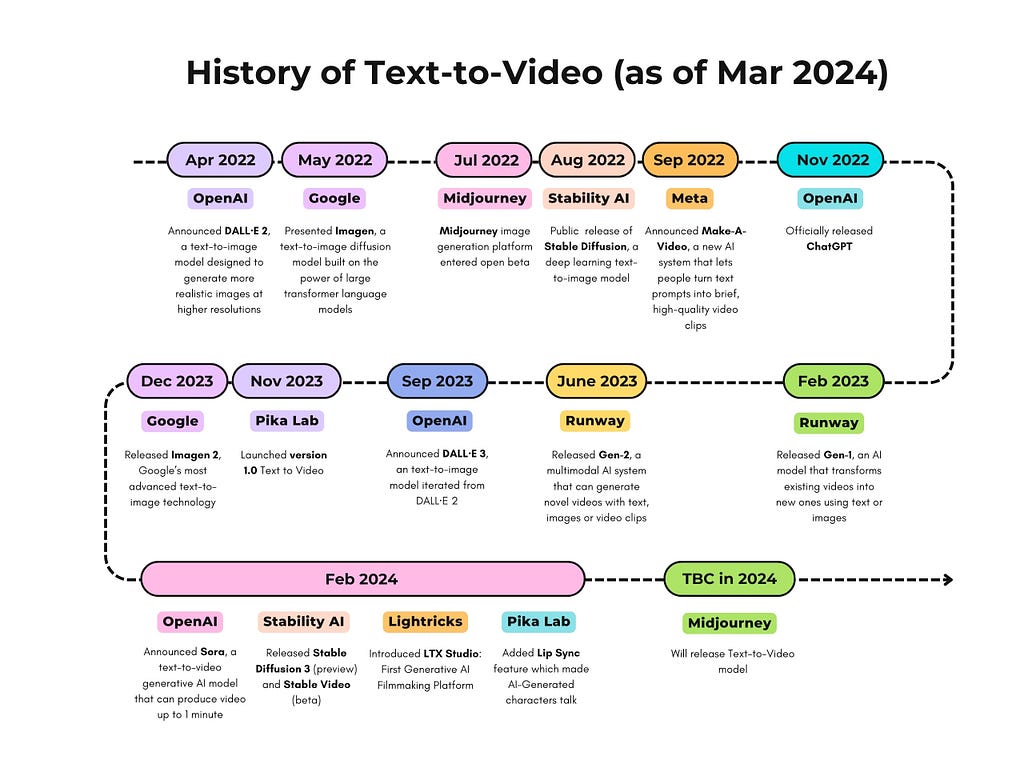

In recent years we have witnessed the emergence of commercial text-to-video models and products. I would like to share a self-created comprehensive timeline diagram that captures the remarkable evolution of commercial text-to-video models / products in the latest 3 years (including 2022, 2023 and 2024 till now).
I created the diagram when preparing for a presentation on Sora to my team. It was exciting to see how such great products emerge along with the development of Computer Vision (CV) research works including but not limited to Generative Adversarial Networks (GANs), transformer architecture and diffusion models.
As suggested by the Microsoft Research paper “Sora: A Review on Background, Technology, Limitations, and Opportunities of Large Vision Models”, we see Sora as leap because it is not just a tool, but also potentially a “world simulator” to simulate physical and contextual dynamics of the depicted scenes in physical world.
This evolution, of course, will not stop and I am sure we will see other exciting news coming in. As a witness I am keen to keep this diagram updated.
I would love to hear your thoughts on this evolution and where you see text-to-video technology heading next. Let’s discuss the impacts, the potential applications, and the ethical considerations that come with these advancements.
Diagram Share: The Evolution of Commercial Text-to-Video was originally published in Towards Data Science on Medium, where people are continuing the conversation by highlighting and responding to this story.
Originally appeared here:
Diagram Share: The Evolution of Commercial Text-to-Video
Go Here to Read this Fast! Diagram Share: The Evolution of Commercial Text-to-Video
Surprise, surprise. It’s not as hard as I thought it would be.
Originally appeared here:
Building Your First Desktop Application using PySide6 [A Data Scientist Edition]