Tag: AI

Posted by Yossi Matias, VP Engineering & Research, and Grey Nearing, Research Scientist, Google Research

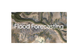
Floods are the most common natural disaster, and are responsible for roughly $50 billion in annual financial damages worldwide. The rate of flood-related disasters has more than doubled since the year 2000 partly due to climate change. Nearly 1.5 billion people, making up 19% of the world’s population, are exposed to substantial risks from severe flood events. Upgrading early warning systems to make accurate and timely information accessible to these populations can save thousands of lives per year.

Driven by the potential impact of reliable flood forecasting on people’s lives globally, we started our flood forecasting effort in 2017. Through this multi-year journey, we advanced research over the years hand-in-hand with building a real-time operational flood forecasting system that provides alerts on Google Search, Maps, Android notifications and through the Flood Hub. However, in order to scale globally, especially in places where accurate local data is not available, more research advances were required.

In “Global prediction of extreme floods in ungauged watersheds”, published in Nature, we demonstrate how machine learning (ML) technologies can significantly improve global-scale flood forecasting relative to the current state-of-the-art for countries where flood-related data is scarce. With these AI-based technologies we extended the reliability of currently-available global nowcasts, on average, from zero to five days, and improved forecasts across regions in Africa and Asia to be similar to what are currently available in Europe. The evaluation of the models was conducted in collaboration with the European Center for Medium Range Weather Forecasting (ECMWF).

These technologies also enable Flood Hub to provide real-time river forecasts up to seven days in advance, covering river reaches across over 80 countries. This information can be used by people, communities, governments and international organizations to take anticipatory action to help protect vulnerable populations.

Flood forecasting at Google

The ML models that power the FloodHub tool are the product of many years of research, conducted in collaboration with several partners, including academics, governments, international organizations, and NGOs.

In 2018, we launched a pilot early warning system in the Ganges-Brahmaputra river basin in India, with the hypothesis that ML could help address the challenging problem of reliable flood forecasting at scale. The pilot was further expanded the following year via the combination of an inundation model, real-time water level measurements, the creation of an elevation map and hydrologic modeling.

In collaboration with academics, and, in particular, with the JKU Institute for Machine Learning we explored ML-based hydrologic models, showing that LSTM-based models could produce more accurate simulations than traditional conceptual and physics-based hydrology models. This research led to flood forecasting improvements that enabled the expansion of our forecasting coverage to include all of India and Bangladesh. We also worked with researchers at Yale University to test technological interventions that increase the reach and impact of flood warnings.

Our hydrological models predict river floods by processing publicly available weather data like precipitation and physical watershed information. Such models must be calibrated to long data records from streamflow gauging stations in individual rivers. A low percentage of global river watersheds (basins) have streamflow gauges, which are expensive but necessary to supply relevant data, and it’s challenging for hydrological simulation and forecasting to provide predictions in basins that lack this infrastructure. Lower gross domestic product (GDP) is correlated with increased vulnerability to flood risks, and there is an inverse correlation between national GDP and the amount of publicly available data in a country. ML helps to address this problem by allowing a single model to be trained on all available river data and to be applied to ungauged basins where no data are available. In this way, models can be trained globally, and can make predictions for any river location.

There is an inverse (log-log) correlation between the amount of publicly available streamflow data in a country and national GDP. Streamflow data from the Global Runoff Data Center.

Our academic collaborations led to ML research that developed methods to estimate uncertainty in river forecasts and showed how ML river forecast models synthesize information from multiple data sources. They demonstrated that these models can simulate extreme events reliably, even when those events are not part of the training data. In an effort to contribute to open science, in 2023 we open-sourced a community-driven dataset for large-sample hydrology in Nature Scientific Data.

The river forecast model

Most hydrology models used by national and international agencies for flood forecasting and river modeling are state-space models, which depend only on daily inputs (e.g., precipitation, temperature, etc.) and the current state of the system (e.g., soil moisture, snowpack, etc.). LSTMs are a variant of state-space models and work by defining a neural network that represents a single time step, where input data (such as current weather conditions) are processed to produce updated state information and output values (streamflow) for that time step. LSTMs are applied sequentially to make time-series predictions, and in this sense, behave similarly to how scientists typically conceptualize hydrologic systems. Empirically, we have found that LSTMs perform well on the task of river forecasting.

A diagram of the LSTM, which is a neural network that operates sequentially in time. An accessible primer can be found here.

Our river forecast model uses two LSTMs applied sequentially: (1) a “hindcast” LSTM ingests historical weather data (dynamic hindcast features) up to the present time (or rather, the issue time of a forecast), and (2) a “forecast” LSTM ingests states from the hindcast LSTM along with forecasted weather data (dynamic forecast features) to make future predictions. One year of historical weather data are input into the hindcast LSTM, and seven days of forecasted weather data are input into the forecast LSTM. Static features include geographical and geophysical characteristics of watersheds that are input into both the hindcast and forecast LSTMs and allow the model to learn different hydrological behaviors and responses in various types of watersheds.

Output from the forecast LSTM is fed into a “head” layer that uses mixture density networks to produce a probabilistic forecast (i.e., predicted parameters of a probability distribution over streamflow). Specifically, the model predicts the parameters of a mixture of heavy-tailed probability density functions, called asymmetric Laplacian distributions, at each forecast time step. The result is a mixture density function, called a Countable Mixture of Asymmetric Laplacians (CMAL) distribution, which represents a probabilistic prediction of the volumetric flow rate in a particular river at a particular time.

LSTM-based river forecast model architecture. Two LSTMs are applied in sequence, one ingesting historical weather data and one ingesting forecasted weather data. The model outputs are the parameters of a probability distribution over streamflow at each forecasted timestep.

Input and training data

The model uses three types of publicly available data inputs, mostly from governmental sources:

1. Static watershed attributes representing geographical and geophysical variables: From the HydroATLAS project, including data like long-term climate indexes (precipitation, temperature, snow fractions), land cover, and anthropogenic attributes (e.g., a nighttime lights index as a proxy for human development).
2. Historical meteorological time-series data: Used to spin up the model for one year prior to the issue time of a forecast. The data comes from NASA IMERG, NOAA CPC Global Unified Gauge-Based Analysis of Daily Precipitation, and the ECMWF ERA5-land reanalysis. Variables include daily total precipitation, air temperature, solar and thermal radiation, snowfall, and surface pressure.
3. Forecasted meteorological time series over a seven-day forecast horizon: Used as input for the forecast LSTM. These data are the same meteorological variables listed above, and come from the ECMWF HRES atmospheric model.

Training data are daily streamflow values from the Global Runoff Data Center over the time period 1980 – 2023. A single streamflow forecast model is trained using data from 5,680 diverse watershed streamflow gauges (shown below) to improve accuracy.

Location of 5,680 streamflow gauges that supply training data for the river forecast model from the Global Runoff Data Center.

Improving on the current state-of-the-art

We compared our river forecast model with GloFAS version 4, the current state-of-the-art global flood forecasting system. These experiments showed that ML can provide accurate warnings earlier and over larger and more impactful events.

The figure below shows the distribution of F1 scores when predicting different severity events at river locations around the world, with plus or minus 1 day accuracy. F1 scores are an average of precision and recall and event severity is measured by return period. For example, a 2-year return period event is a volume of streamflow that is expected to be exceeded on average once every two years. Our model achieves reliability scores at up to 4-day or 5-day lead times that are similar to or better, on average, than the reliability of GloFAS nowcasts (0-day lead time).

Distributions of F1 scores over 2-year return period events in 2,092 watersheds globally during the time period 2014-2023 from GloFAS (blue) and our model (orange) at different lead times. On average, our model is statistically as accurate as GloFAS nowcasts (0–day lead time) up to 5 days in advance over 2-year (shown) and 1-year, 5-year, and 10-year events (not shown).

Additionally (not shown), our model achieves accuracies over larger and rarer extreme events, with precision and recall scores over 5-year return period events that are similar to or better than GloFAS accuracies over 1-year return period events. See the paper for more information.

Looking into the future

The flood forecasting initiative is part of our Adaptation and Resilience efforts and reflects Google’s commitment to address climate change while helping global communities become more resilient. We believe that AI and ML will continue to play a critical role in helping advance science and research towards climate action.

We actively collaborate with several international aid organizations (e.g., the Centre for Humanitarian Data and the Red Cross) to provide actionable flood forecasts. Additionally, in an ongoing collaboration with the World Meteorological Organization (WMO) to support early warning systems for climate hazards, we are conducting a study to help understand how AI can help address real-world challenges faced by national flood forecasting agencies.

While the work presented here demonstrates a significant step forward in flood forecasting, future work is needed to further expand flood forecasting coverage to more locations globally and other types of flood-related events and disasters, including flash floods and urban floods. We are looking forward to continuing collaborations with our partners in the academic and expert communities, local governments and the industry to reach these goals.

How the Bud Light boycott and SalesForce’s innovation plans confuse the best LLMs

Can the best AI models today, accurately pick up the most important message out of a company earnings call? They can certainly pick up SOME points but how do we know if those are the important ones? Can we prompt them into to doing a better job? To find those answers, we look at what the best journalists in the field have done and try to get as close to that with AI

The Challenge

In this article, I look at 8 recent company earnings calls and ask the current contestants for smartest AIs (Claude 3, GPT-4 and Mistral Large) what they think is important. Then compare the results to what some of the best names in Journalism (Reuters, Bloomberg, and Barron’s) have said about those exact reports.

Why care about this?

The Significance of Earnings Calls

Earnings calls are quarterly events where senior management reviews the company’s financial results. They discuss the company’s performance, share commentary, and sometimes preview future plans. These discussions can significantly impact the company’s stock price. Management explains their future expectations and reasons for meeting or surpassing past forecasts. The management team offers invaluable insights into the company’s actual condition and future direction.

The Power of Automation in Earnings Analysis

Statista reports that there are just under 4000 companies listed on the NASDAQ and about 58,000 globally according to one estimate.

A typical conference call lasts roughly 1 hour. To just listen to all NASDAQ companies, one would need at least 10 people working full-time for the entire quarter. And this doesn’t even include the more time-consuming tasks like analyzing and comparing financial reports.

Large brokerages might manage this workload, but it’s unrealistic for individual investors. Automation in this area could level the playing field, making it easier for everyone to understand quarterly earnings.

While this may just be within reach of large brokerages, it is not feasible for private investors. Therefore, any reliable automation in this space will be a boon, especially for democratizing the understanding of quarterly earnings.

The Process of Testing AI as a Financial Analyst

To test how well the best LLMs of the day can do this job. I decided to compare the main takeaways by humans and see how well AI can mimic that. Here are the steps:

1. Pick some companies with recent earnings call transcripts and matching news articles.
2. Provide the LLMs with the full transcript as context and ask them to provide the top three bullet points that seem most impactful for the value of the company. This is important as, providing a longer summary becomes progressively easier — there are only so many important things to say.
3. To ensure we maximise the quality of the output, I vary the way I phrase the problem to the AI (using different prompts): Ranging from simply asking for a summary, adding more detailed instructions, adding previous transcripts and some combinations of those.
4. Finally, compare those with the 3 most important points from the respective news article and use the overlap as a measure of success.

Summary of Results

GPT-4 shows best performance at 80% when providing it the previous quarter’s transcript and using a set of instructions on how to analyse transcripts well (Chain of Thought). Notably, just using correct instructions increases GPT-4 performance from 51% to 75%.

• Next best performers are:
   — Claude 3 Opus (67%) — Without sophisticated prompting, Claude 3 Opus works best.
   — Mistral Large (66%) when adding supporting instructions (i.e. Chain of Thought)
• Chain-of-thought (CoT) and Think Step by Step (SxS) seem to work well for GPT-4 but are detrimental for other models. This suggests there is still a lot to be learned about what prompts work for each LLM.
• Chain-of-Thought (CoT) seems almost always outperforms Step-by-step (SxS). This means tailored financial knowledge of priorities for analysis helps. The specific instructions provided are listed at the bottom of the article.
• More data-less sense: Adding a previous period transcript to the model context seems to be at least slightly and at worst significantly detrimental to results across the board than just focusing on the latest results (except for GPT-4 + CoT). Potentially, there is much irrelevant information introduced from a previous transcript and a relatively small amount of specific facts to make a quarter-on-quarter comparison. Mistral Large’s performance drops significantly, note that its context window is just 32k tokens vs the significantly larger ones for the others (2 transcripts + prompt actually just barely fit under 32k tokens).
• Claude-3 Opus and Sonnet perform very closely, with Sonnet actually outperforming Opus in some cases. However, this tends to be by a few %-age points and can therefore be attributed to the randomness of results.
• Note that, as mentioned, results show a high degree of variability and the range of outcomes is within +/-6%. For that reason, I have rerun all analysis 3 times and am showing the averages. However, the +/-6% range is not sufficient to significantly upend any of the above conclusions

What do LLMs get right and wrong?

How the Bud Light Boycott and Salesforce’s AI plans confused the best AIs

This task offers some easy wins: guessing that results are about the latest revenue numbers and next year’s projections is fairly on the nose. Unsurprisingly, this is where models get things right most of the time.

The table below gives an overview of what was mentioned in the news and what LLMs chose differently when summarized in just a few words.

Next, I tried to look for any trends of what the models consistently miss. Those generally Fall into a few categories:

• Making sense of changes: In the above results, LLMs have been able to understand fairly reliably what to look for: earnings, sales, dividend, and guidance, however, making sense of what is significant is still very elusive. For instance, common-sense might suggest that Q4 2023 results will be a key topic for any company and this is what the LLMs pick. However, Nordstrom talks about muted revenue and demand expectations for 2024 which pushes Q4 2023 results aside in terms of importance
• Hallucinations: as is well documented, LLMs tend to make up facts. In this case, despite having instructions to “only include facts and metrics from the context” some metrics and dates end up being made up. The models unfortunately will not be shy about talking about the Q4 2024 earnings by referring to them as already available and using the 2023 numbers for them.
• Significant one-off events: Unexpected one-off events are surprisingly often missed by LLMs. For instance, the boycott of Bud Light drove sales of the best-selling beer in the US down by 15.9% for Anheuser-Busch and is discussed at length in the transcripts. The number alone should appear significant, however it was missed by all models in the sample.
• Actions speak louder than words: Both GPT and Claude highlight innovation and the commitment to AI as important.
   — Salesforce (CRM) talks at length about a heavy focus on AI and Data Cloud
   — Snowflake appointed their SVP of AI and former exec of Google Ads as CEO (Sridhar Ramaswamy), similarly signaling a focus on leveraging AI technology.
  Both signal a shift to innovation & AI. However, journalists and analysts are not as easily tricked into mistaking words for actions. In the article analyzing CRM’s earnings, the subtitle reads Salesforce Outlook Disappoints as AI Fails to Spark Growth. However, Salesforce has been trying to tango with AI for a while and the forward-looking plans to use AI are not even mentioned. Salesforce’s transcript mentions AI 91 times while Snowflake’s less than half of that at 39. However, humans can make the distinction in meaning: Bloomberg’s article [link] on the appointment of a new CEO: His elevation underscores a focus on AI for Snowflake.

Experiment design and choices

1. Why Earnings call transcripts? The more intuitive choice may be company filings, however, I find transcripts to present a more natural and less formal discussion of events. I believe transcripts give the LLM as a reasoning engine a better chance to glean more natural commentary of events as opposed to the dry and highly regulated commentary of earnings. The calls are mostly management presentations, which might skew things toward a more positive view. However, my analysis has shown the performance of the LLMs seems similar between positive and negative narratives.
2. Choice of Companies: I chose stocks that have published Q4 2023 earnings reports between 25 Feb and 5 March and have been reported on by one of Reuters, Bloomberg, or Barron’s. This ensures that the results are timely and that the models have not been trained on that data yet. Plus, everyone always talks about AAPL and TSLA, so this is something different. Finally, the reputation of these journalistic houses ensures a meaningful comparison. The 8 stocks we ended up with are: Autodesk (ADSK), BestBuy (BBY), Anheuser-Busch InBev (BUD), Salesforce (CRM), DocuSign (DOCU), Nordstrom (JWN), Kroger (KR), Snowflake (SNOW)
3. Variability of results LLM results can vary between runs so I have run all experiments 3 times and show an average. All analysis for all models was done using temperature 0 which is commonly used to minimize variation of results. In this case, I have observed different runs have as much as 10% difference in performance. This is due to the small sample (only 24 data points 8 stocks by 3 statements) and the fact that we are basically asking an LLM to choose one of many possible statements for the summary, so when this happens with some randomness it can naturally lead to picking some of them differently.
4. Choice of Prompts: For each of the 3 LLMs in comparison try out 4 different prompting approaches:

• Naive — The prompt simply asks the model to determine the most likely impact on the share price.
• Chain-of-Thought (CoT) — where I provide a detailed list of steps to follow when choosing a summary. This is inspired and loosely follows [Wei et. al. 2022] work outlining the Chain of Thought approach, providing reasoning steps as part of the prompt dramatically improves results. These additional instructions, in the context of this experiment, include typical drivers of price movements: changes to expected performance in revenue, costs, earnings, litigation, etc.
• Step by Step (SxS) aka Zero-shot CoT, inspired by Kojima et.al (2022) where they discovered that simply adding the phrase “Let’s think step by step” improves performance. I ask the LLMs to think step-by-step and describe their logic before answering.
• Previous transcript — finally, I run all three of the above prompts once more by including the transcript from the previous quarter (in this case Q3)

Conclusion

From what we can see above, Journalists’ and Research Analysts’ jobs seem safe for now, as most LLMs struggle to get more than two of three answers correctly. In most cases, this just means guessing that the meeting was about the latest revenue and next year’s projections.

However, despite all the limitations of this test, we can still see some clear conclusions:

• The accuracy level is fairly low for most models. Even GPT-4’s best performance of 80% will be problematic at scale without human supervision — giving wrong advice one in five times is not convincing.
• GPT4 seems to still be a clear leader in complex tasks it was not specifically trained for.
• There are significant gains when correctly prompt engineering the task
• Most models seem easily confused by extra information as adding the previous transcript generally reduces performance.

Where to from here?

We have all witnessed that LLM capabilities continuously improve. Will this gap be closed and how? We have observed three types of cognitive issues that have impacted performance: hallucinations, understanding what is important and what isn’t (e.g. really understanding what is surprising for a company), more complex company causality issues (e.g. like the Bud Light boycott and how important the US sales are relative to an overall business):

• Hallucinations or scenarios where the LLM cannot correctly reproduce factual information are a major stumbling block in applications that require strict adherence to factuality. Advanced RAG approaches, combined with research in the area continue to make progress, [Huang et al 2023] give an overview of current progress
• Understanding what is important — fine-tuning LLM models for the specific use case should lead to some improvements. However, those come with much bigger requirements on team, cost, data, and infrastructure.
• Complex Causality Links — this one may be a good direction for AI Agents. For instance, in the Bud Light boycott case, the model might need to:
  1. the importance of Bud Light to US sales, which is likely peppered through many presentations and management commentary
  2. The importance of US sales ot the overall company, which could be gleaned from company financials
  3. Finally stack those impacts to all other impacts mentioned
  Such causal logic is more akin to how a ReAct AI Agent might think instead of just a standalone LLM [Yao, et al 2022]. Agent planning is a hot research topic [Chen, et al 2024]

Follow me on LinkedIn

Disclaimers

The views, opinions, and conclusions expressed in this article are my own and do not reflect the views or positions of any of the entities mentioned or any other entities.

No data was used to model training nor was systematically collected from the sources mentioned, all techniques were limited to prompt engineering.

Resources

Earnings Call Transcripts (Motley Fool)

• Anheuser-Busch InBev (BUD) Q4 2024
• Autodesk (ADSK) Q4 2024
• Best Buy (BBY) Q4 2024
• DocuSign (DOCU) Q4 2024
• Kroger (KR) Q4 2024
• Nordstrom (JWN) Q4 2024
• Salesforce (CRM) Q4 2024
• Snowflake (SNOW) Q4 2024

News Articles

• Anheuser-Busch InBev (Reuters)
• Autodesk (Reuters)
• BestBuy (Bloomberg)
• DocuSign (Barron’s)
• Kroger (Barron’s)
• Nordstrom (Bloomberg)
• Salesforce (Bloomberg)
• Snowflake (Bloomberg)

---

AI vs. Human Insight in Financial Analysis was originally published in Towards Data Science on Medium, where people are continuing the conversation by highlighting and responding to this story.

Explore what exactly happens behind-the-scenes in Vector Databases

The other day I asked my favorite Large Language Model (LLM) to help me explain vectors to my almost 4-year old. In seconds, it spit out a story filled with mythical creatures and magic and vectors. And Voila! I had a sketch for a new children’s book, and it was impressive because the unicorn was called ‘LuminaVec’.

So, how did the model help weave this creative magic? Well, the answer is by using vectors (in real life) and most probably vector databases. How so? Let me explain.

Vectors and Embedding

First, the model doesn’t understand the exact words I typed in. What helps it understand the words are their numerical representations which are in the form of vectors. These vectors help the model find similarity among the different words while focusing on meaningful information about each. It does this by using embeddings which are low-dimensional vectors that try to capture the semantics and context of the information.

In other words, vectors in an embedding are lists of numbers that specify the position of an object with respect to a reference space. These objects can be features that define a variable in a dataset. With the help of these numerical vector values, we can determine how close or how far one feature is from the other — are they similar (close) or not similar (far)?

Now these vectors are quite powerful but when we are talking about LLMs, we need to be extra cautious about them because of the word ‘large’. As it happens to be with these ‘large’ models, these vectors may quickly become long and more complex, spanning over hundreds or even thousands of dimensions. If not dealt with carefully, the processing speed and mounting expense could become cumbersome very fast!

Vector Databases

To address this issue, we have our mighty warrior : Vector databases.

Vector databases are special databases that contain these vector embeddings. Similar objects have vectors that are closer to each other in the vector database, while dissimilar objects have vectors that are farther apart. So, rather than parsing the data every time a query comes in and generating these vector embeddings, which induces huge resources, it is much faster to run the data through the model once, store it in the vector database and retrieve it as needed. This makes vector databases one of the most powerful solutions addressing the problem of scale and speed for these LLMs.

So, going back to the story about the rainbow unicorn, sparkling magic and powerful vectors — when I had asked the model that question, it may have followed a process as this –

1. The embedding model first transformed the question to a vector embedding.
2. This vector embedding was then compared to the embeddings in the vector database(s) related to fun stories for 5-year olds and vectors.
3. Based on this search and comparison, the vectors that were the most similar were returned. The result should have consisted of a list of vectors ranked in their order of similarity to the query vector.

How does it really work?

To distill things even further, how about we go on a ride to resolve these steps on the micro-level? Time to go back to the basics! Thanks to Prof. Tom Yeh, we have this beautiful handiwork that explains the behind-the-scenes workings of the vectors and vector databases. (All the images below, unless otherwise noted, are by Prof. Tom Yeh from the above-mentioned LinkedIn post, which I have edited with his permission. )

So, here we go:

For our example, we have a dataset of three sentences with 3 words (or tokens) for each.

• How are you
• Who are you
• Who am I

And our query is the sentence ‘am I you’.

In real life, a database may contain billions of sentences (think Wikipedia, news archives, journal papers, or any collection of documents) with tens of thousands of max number of tokens. Now that the stage is set, let the process begin :

[1] Embedding : The first step is generating vector embeddings for all the text that we want to be using. To do so, we search for our corresponding words in a table of 22 vectors, where 22 is the vocabulary size for our example.

In real life, the vocabulary size can be tens of thousands. The word embedding dimensions are in the thousands (e.g., 1024, 4096).

By searching for the words how are you in the vocabulary, the word embedding for it looks as this:

[2] Encoding : The next step is encoding the word embedding to obtain a sequence of feature vectors, one per word. For our example, the encoder is a simple perceptron consisting of a Linear layer with a ReLU activation function.

A quick recap:

Linear transformation : The input embedding vector is multiplied by the weight matrix W and then added with the bias vector b,

z = Wx+b, where W is the weight matrix, x is our word embedding and b is the bias vector.

ReLU activation function : Next, we apply the ReLU to this intermediate z.

ReLU returns the element-wise maximum of the input and zero. Mathematically, h = max{0,z}.

Thus, for this example the text embedding looks like this:

To show how it works, let’s calculate the values for the last column as an example.

Linear transformation :

[1.0 + 1.1 + 0.0 +0.0] + 0 = 1

[0.0 + 1.1 + 0.0 + 1.0] + 0 = 1

[1.0 + (0).1+ 1.0 + 0.0] + (-1) = -1

[1.0 + (-1).1+ 0.0 + 0.0] + 0 = -1

ReLU

max {0,1} =1

max {0,1} = 1

max {0,-1} = 0

max {0,-1} = 0

And thus we get the last column of our feature vector. We can repeat the same steps for the other columns.

[3] Mean Pooling : In this step, we club the feature vectors by averaging over the columns to obtain a single vector. This is often called text embedding or sentence embedding.

Other techniques for pooling such as CLS, SEP can be used but Mean Pooling is the one used most widely.

[4] Indexing : The next step involves reducing the dimensions of the text embedding vector, which is done with the help of a projection matrix. This projection matrix could be random. The idea here is to obtain a short representation which would allow faster comparison and retrieval.

This result is kept away in the vector storage.

[5] Repeat : The above steps [1]-[4] are repeated for the other sentences in the dataset “who are you” and “who am I”.

Now that we have indexed our dataset in the vector database, we move on to the actual query and see how these indices play out to give us the solution.

Query : “am I you”

[6] To get started, we repeat the same steps as above — embedding, encoding and indexing to obtain a 2d-vector representation of our query.

[7] Dot Product (Finding Similarity)

Once the previous steps are done, we perform dot products. This is important as these dot products power the idea of comparison between the query vector and our database vectors. To perform this step, we transpose our query vector and multiply it with the database vectors.

[8] Nearest Neighbor

The final step is performing a linear scan to find the largest dot product, which for our example is 60/9. This is the vector representation for “who am I”. In real life, a linear scan could be incredibly slow as it may involve billions of values, the alternative is to use an Approximate Nearest Neighbor (ANN) algorithm like the Hierarchical Navigable Small Worlds (HNSW).

And that brings us to the end of this elegant method.

Thus, by using the vector embeddings of the datasets in the vector database, and performing the steps above, we were able to find the sentence closest to our query. Embedding, encoding, mean pooling, indexing and then dot products form the core of this process.

The ‘large’ picture

However, to bring in the ‘large’ perspective one more time –

• A dataset may contain millions or billions of sentences.
• The number of tokens for each of them can be tens of thousands.
• The word embedding dimensions can be in the thousands.

As we put all of these data and steps together, we are talking about performing operations on dimensions that are mammoth-like in size. And so, to power through this magnificent scale, vector databases come to the rescue. Since we started this article talking about LLMs, it would be a good place to say that because of the scale-handling capability of vector databases, they have come to play a significant role in Retrieval Augmented Generation (RAG). The scalability and speed offered by vector databases enable efficient retrieval for the RAG models, thus paving the way for an efficient generative model.

All in all it is quite right to say that vector databases are powerful. No wonder they have been here for a while — starting their journey of helping recommendation systems to now powering the LLMs, their rule continues. And with the pace vector embeddings are growing for different AI modalities, it seems like vector databases are going to continue their rule for a good amount of time in the future!

P.S. If you would like to work through this exercise on your own, here is a link to a blank template for your use.

Blank Template for hand-exercise

Now go have fun and create some ‘luminous vectoresque’ magic!

---

Deep Dive into Vector Databases by Hand ✍︎ was originally published in Towards Data Science on Medium, where people are continuing the conversation by highlighting and responding to this story.

Building Ethical AI Starts with the Data Team — Here’s Why

GenAI is an ethical quagmire. What responsibility do data leaders have to navigate it? In this article, we consider the need for ethical AI and why data ethics are AI ethics.

When it comes to the technology race, moving quickly has always been the hallmark of future success.

Unfortunately, moving too quickly also means we can risk overlooking the hazards waiting in the wings.

It’s a tale as old as time. One minute you’re sequencing prehistoric mosquito genes, the next minute you’re opening a dinosaur theme park and designing the world’s first failed hyperloop (but certainly not the last).

When it comes to GenAI, life imitates art.

No matter how much we might like to consider AI a known quantity, the harsh reality is that not even the creators of this technology are totally sure how it works.

After multiple high profile AI snafus from the likes of United Healthcare, Google, and even the Canadian courts, it’s time to consider where we went wrong.

Now, to be clear, I believe GenAI (and AI more broadly) will eventually be critical to every industry — from expediting engineering workflows to answering common questions. However, in order to realize the potential value of AI, we’ll first have to start thinking critically about how we develop AI applications — and the role data teams play in it.

In this post, we’ll look at three ethical concerns in AI, how data teams are involved, and what you as a data leader can do today to deliver more ethical and reliable AI for tomorrow.

The Three Layers of AI Ethics

When I was chatting with my colleague Shane Murray, the former New York Times SVP of Data & Insights, he shared one of the first times he was presented with a real ethical quandary. While developing an ML model for financial incentives at the New York Times, the discussion was raised about the ethical implications of a machine learning model that could determine discounts.

On its face, an ML model for discount codes seemed like a pretty innocuous request all things considered. But as innocent as it might have seemed to automate away a few discount codes, the act of removing human empathy from that business problem created all kinds of ethical considerations for the team.

The race to automate simple but traditionally human activities seems like an exclusively pragmatic decision — a simple binary of improving or not improving efficiency. But the second you remove human judgment from any equation, whether an AI is involved or not, you also lose the ability to directly manage the human impact of that process.

That’s a real problem.

When it comes to the development of AI, there are three primary ethical considerations:

1. Model Bias

This gets to the heart of our discussion at the New York Times. Will the model itself have any unintended consequences that could advantage or disadvantage one person over another?

The challenge here is to design your GenAI in such a way that — all other considerations being equal — it will consistently provide fair and impartial outputs for every interaction.

2. AI Usage

Arguably the most existential — and interesting — of the ethical considerations for AI is understanding how the technology will be used and what the implications of that use-case might be for a company or society more broadly.

Was this AI designed for an ethical purpose? Will its usage directly or indirectly harm any person or group of people? And ultimately, will this model provide net good over the long-term?

As it was so poignantly defined by Dr. Ian Malcolm in the first act of Jurassic Park, just because you can build something doesn’t mean you should.

3. Data Responsibility

And finally, the most important concern for data teams (as well as where I’ll be spending the majority of my time in this piece): how does the data itself impact an AI’s ability to be built and leveraged responsibly?

This consideration deals with understanding what data we’re using, under what circumstances it can be used safely, and what risks are associated with it.

For example, do we know where the data came from and how it was acquired? Are there any privacy issues with the data feeding a given model? Are we leveraging any personal data that puts individuals at undue risk of harm?

Is it safe to build on a closed-source LLM when you don’t know what data it’s been trained on?

And, as highlighted in the lawsuit filed by the New York Times against OpenAI — do we have the right to use any of this data in the first place?

This is also where the quality of our data comes into play. Can we trust the reliability of data that’s feeding a given model? What are the potential consequences of quality issues if they’re allowed to reach AI production?

So, now that we’ve taken a 30,000-foot look at some of these ethical concerns, let’s consider the data team’s responsibility in all this.

Why Data Teams Are Responsible for AI Ethics

Of all the ethical AI considerations adjacent to data teams, the most salient by far is the issue of data responsibility.

In the same way GDPR forced business and data teams to work together to rethink how data was being collected and used, GenAI will force companies to rethink what workflows can — and can’t — be automated away.

While we as data teams absolutely have a responsibility to try to speak into the construction of any AI model, we can’t directly affect the outcome of its design. However, by keeping the wrong data out of that model, we can go a long way toward mitigating the risks posed by those design flaws.

And if the model itself is outside our locus of control, the existential questions of can and should are on a different planet entirely. Again, we have an obligation to point out pitfalls where we see them, but at the end of the day, the rocket is taking off whether we get on board or not.
The most important thing we can do is make sure that the rocket takes off safely. (Or steal the fuselage.)

So — as in all areas of the data engineer’s life — where we want to spend our time and effort is where we can have the greatest direct impact for the greatest number of people. And that opportunity resides in the data itself.

Why Data Responsibility Should Matter to the Data Team

It seems almost too obvious to say, but I’ll say it anyway:

Data teams need to take responsibility for how data is leveraged into AI models because, quite frankly, they’re the only team that can. Of course, there are compliance teams, security teams, and even legal teams that will be on the hook when ethics are ignored. But no matter how much responsibility can be shared around, at the end of the day, those teams will never understand the data at the same level as the data team.

Imagine your software engineering team creates an app using a third-party LLM from OpenAI or Anthropic, but not realizing that you’re tracking and storing location data — in addition to the data they actually need for their application — they leverage an entire database to power the model. With the right deficiencies in logic, a bad actor could easily engineer a prompt to track down any individual using the data stored in that dataset. (This is exactly the tension between open and closed source LLMs.)

Or let’s say the software team knows about that location data but they don’t realize that location data could actually be approximate. They could use that location data to create AI mapping technology that unintentionally leads a 16-year-old down a dark alley at night instead of the Pizza Hut down the block. Of course, this kind of error isn’t volitional, but it underscores the unintended risks inherent to how the data is leveraged.

These examples and others highlight the data team’s role as the gatekeeper when it comes to ethical AI.

So, how can data teams remain ethical?

In most cases, data teams are used to dealing with approximate and proxy data to make their models work. But when it comes to the data that feeds an AI model, you actually need a much higher level of validation.

To effectively stand in the gap for consumers, data teams will need to take an intentional look at both their data practices and how those practices relate to their organization at large.

As we consider how to mitigate the risks of AI, below are 3 steps data teams must take to move AI toward a more ethical future.

1. Get a seat at the table

Data teams aren’t ostriches — they can’t bury their heads in the sand and hope the problem goes away. In the same way that data teams have fought for a seat at the leadership table, data teams need to advocate for their seat at the AI table.

Like any data quality fire drill, it’s not enough to jump into the fray after the earth is already scorched. When we’re dealing with the type of existential risks that are so inherent to GenAI, it’s more important than ever to be proactive about how we approach our own personal responsibility.

And if they won’t let you sit at the table, then you have a responsibility to educate from the outside. Do everything in your power to deliver excellent discovery, governance, and data quality solutions to arm those teams at the helm with the information to make responsible decisions about the data. Teach them what to use, when to use it, and the risks of using third-party data that can’t be validated by your team’s internal protocols.

This isn’t just a business issue. As United Healthcare and the province of British Columbia can attest, in many cases, these are real peoples lives — and livelihoods — on the line. So, let’s make sure we’re operating with that perspective.

2. Leverage methodologies like RAG to curate more responsible — and reliable — data

We often talk about retrieval augmented generation (RAG) as a resource to create value from an AI. But it’s also just as much a resource to safeguard how that AI will be built and used.

Imagine for example that a model is accessing private customer data to feed a consumer-facing chat app. The right user prompt could send all kinds of critical PII spilling out into the open for bad actors to seize upon. So, the ability to validate and control where that data is coming from is critical to safeguarding the integrity of that AI product.

Knowledgeable data teams mitigate a lot of that risk by leveraging methodologies like RAG to carefully curate compliant, safer and more model-appropriate data.

Taking a RAG-approach to AI development also helps to minimize the risk associated with ingesting too much data — as referenced in our location-data example.

So what does that look like in practice? Let’s say you’re a media company like Netflix that needs to leverage first-party content data with some level of customer data to create a personalized recommendation model. Once you define what the specific — and limited — data points are for that use case, you’ll be able to more effectively define:

1. Who’s responsible for maintaining and validating that data,
2. Under what circumstances that data can be used safely,
3. And who’s ultimately best suited to build and maintain that AI product over time.

Tools like data lineage can also be helpful here by enabling your team to quickly validate the origins of your data as well as where it’s being used — or misused — in your team’s AI products over time.

3. Prioritize data reliability

When we’re talking about data products, we often say “garbage in, garbage out,” but in the case of GenAI, that adage falls a hair short. In reality, when garbage goes into an AI model, it’s not just garbage that comes out — it’s garbage plus real human consequences as well.

That’s why, as much as you need a RAG architecture to control the data being fed into your models, you need robust data observability that connects to vector databases like Pinecone to make sure that data is actually clean, safe, and reliable.

One of the most common complaints I’ve heard from customers getting started with AI is that pursuing production-ready AI is that if you’re not actively monitoring the ingestion of indexes into the vector data pipeline, it’s nearly impossible to validate the trustworthiness of the data.

More often than not, the only way data and AI engineers will know that something went wrong with the data is when that model spits out a bad prompt response — and by then, it’s already too late.

There’s no time like the present

The need for greater data reliability and trust is the very same challenge that inspired our team to create the data observability category in 2019.

Today, as AI promises to upend many of the processes and systems we’ve come to rely on day-to-day, the challenges — and more importantly, the ethical implications — of data quality are becoming even more dire.

---

Building Ethical AI Starts with the Data Team — Here’s Why was originally published in Towards Data Science on Medium, where people are continuing the conversation by highlighting and responding to this story.

This tutorial will teach you how to create sparse and dense embeddings and build a recommender system using hybrid search

This tutorial provides a step-by-step guide with code on how to create a chatbot-style recommender system. By the end, you will have built a recommender that uses the user’s open-text input to find matching items through a hybrid search on sparse and dense vectors. The dataset used in this tutorial contains recipes. However, you can easily replace the dataset with one that suits your needs with minimal adjustments. The first part of this task will focus on building the recommender system, which involves data cleaning, creating sparse and dense embeddings, uploading them to a vector database, and performing dense vector search and hybrid search. In the second part, you will create a chatbot that generates responses based on user input and recommendations, and a UI using a Plotly dashboard.

To follow this tutorial, you will need to set up accounts for paid services such as Vertex AI, OpenAI API, and Pinecone. Fortunately, most services offer free credits, and the costs associated with this tutorial should not exceed $5. Additionally, you can reduce costs further by using the files and datasets provided on my GitHub repository.

Data preparation

For this project, we will use recipes from Public Domain Recipes. All recipes are stored as markdown files in this GitHub repository. For this tutorial, I already did some data cleaning and created features from the raw text input. If you are keen on doing the data cleaning part yourself, the code is available on my GitHub repository.

The dataset consists of the following columns:

• title: the title of the recipe
• date: the date the recipe was added
• tags: a list of tags that describe the meal
• introduction: an introduction to the recipe, the content varies strongly between records
• ingredients: all needed ingredients. Note that I removed the quantity as it is not needed for creating embeddings and contrary may lead to undesirable recommendations.
• direction: all required steps you need to perform to cook the meal
• recipe_type: indicator if the recipe is vegan, vegetarian, or regular
• output: contains the title, ingredients, and direction of the recipe and will be later provided to the chat model as input.

Let’s have a look at the distribution of the recipe_type feature. We see that the majority (60%) of the recipes include fish or meat and aren’t vegetarian-friendly. Approximately 35% are vegetarian-friendly and only 5% are vegan-friendly. This feature will be used as a hard filter for retrieving matching recipes from the vector database.

import re
import json
import spacy
import torch
import openai
import vertexai
import pandas as pd
import numpy as np
import matplotlib.pyplot as plt
from tqdm.auto import tqdm
from transformers import AutoModelForMaskedLM, AutoTokenizer
from pinecone import Pinecone, ServerlessSpec
from vertexai.language_models import TextEmbeddingModel
from utils_google import authenticate
credentials, PROJECT_ID, service_account, pinecone_API_KEY = authenticate() 
from utils_openai import authenticate
OPENAI_API_KEY = authenticate() 

openai_client = openai.OpenAI(api_key=OPENAI_API_KEY)

REGION = "us-central1"
vertexai.init(project = PROJECT_ID,
              location = REGION,
              credentials = credentials)

pc = Pinecone(api_key=pinecone_API_KEY)

# download spacy model
#!python -m spacy download en_core_web_sm

recipes = pd.read_json("recipes_v2.json")
recipes.head()

plt.bar(recipes.recipe_type.unique(), recipes.recipe_type.value_counts(normalize=True).values)
plt.show()

Hybrid search uses a combination of sparse and dense vectors and a weighting factor alpha, which allows adjusting the importance of the dense vector in the retrieval process. In the following, we will create dense vectors based on the title, tags, and introduction and sparse vectors on the ingredients. By adjusting alpha we can therefore later on determine how much “attention” should be paid to ingredients the user mentioned in its query.

Before creating the embeddings a new feature needs to be created that contains the combined information of the title, the tags, and the introduction.

recipes["dense_feature"] = recipes.title + "; " + recipes.tags.apply(lambda x: str(x).strip("[]").replace("'", "")) + "; " + recipes.introduction
recipes["dense_feature"].head()

Finally, before diving deeper into the generation of the embeddings we’ll have a look at the output column. The second part of the tutorial will be all about creating a chatbot using OpenAI that is able to answer user questions using knowledge from our recipe database. Therefore, after finding the recipes that match best the user query the chat model needs some information it builds its answer on. That’s where the output is used, as it contains all the needed information for an adequate answer

# example output
{'title': 'Creamy Mashed Potatoes',
 'ingredients': 'The quantities here are for about four adult portions. If you are planning on eating this as a side dish, it might be more like 6-8 portions. * 1kg potatoes * 200ml milk* * 200ml mayonnaise* * ~100g cheese * Garlic powder * 12-16 strips of bacon * Butter * 3-4 green onions * Black pepper * Salt  *You can play with the proportions depending on how creamy or dry you want the mashed potatoes to be.',
 'direction': '1. Peel and cut the potatoes into medium sized pieces. 2. Put the potatoes in a pot with some water so that it covers the potatoes and   boil them for about 20-30 minutes, or until the potatoes are soft. 3. About ten minutes before removing the potatoes from the boiling water, cut   the bacon into little pieces and fry it. 4. Warm up the milk and mayonnaise. 5. Shred the cheese. 6. When the potatoes are done, remove all water from the pot, add the warm milk   and mayonnaise mix, add some butter, and mash with a potato masher or a   blender. 7. Add some salt, black pepper and garlic powder to taste and continue mashing   the mix. 8. Once the mix is somewhat homogeneous and the potatoes are properly mashed,   add the shredded cheese and fried bacon and mix a little. 9. Serve and top with chopped green onions.'}

Further, a unique identifier needs to be added to each recipe, which allows retrieving the records of the recommended candidate recipes and their output.

recipes["ID"] = range(len(recipes))

Generate sparse embeddings

The next step involves creating sparse embeddings for all 360 observations. To calculate these embeddings, a more sophisticated method than the frequently used TF-IDF or BM25 approach is used. Instead, the SPLADE Sparse Lexical and Expansion model is applied. A detailed explanation of SPLADE can be found here. Dense embeddings have the same shape for each text input, regardless of the number of tokens in the input. In contrast, sparse embeddings contain a weight for each unique token in the input. The dictionary below represents a sparse vector, where the token ID is the key and the assigned weight is the value.

model_id = "naver/splade-cocondenser-ensembledistil"

tokenizer = AutoTokenizer.from_pretrained(model_id)
model = AutoModelForMaskedLM.from_pretrained(model_id)

def to_sparse_vector(text, tokenizer, model):
    tokens = tokenizer(text, return_tensors='pt')
    output = model(**tokens)
    vec = torch.max(
        torch.log(1 + torch.relu(output.logits)) * tokens.attention_mask.unsqueeze(-1), dim=1
    )[0].squeeze()

    cols = vec.nonzero().squeeze().cpu().tolist()
    weights = vec[cols].cpu().tolist()
    sparse_dict = dict(zip(cols, weights))
    return sparse_dict
    
sparse_vectors = []

for i in tqdm(range(len(recipes))):
    sparse_vectors.append(to_sparse_vector(recipes.iloc[i]["ingredients"], tokenizer, model))

recipes["sparse_vectors"] = sparse_vectors

Generating dense embeddings

At this point of the tutorial, some costs will arise if you use a text embedding model from VertexAI (Google) or OpenAI. However, if you use the same dataset, the costs will be at most $5. The cost may vary if you use a dataset with more records or longer texts, as you are charged by tokens. If you do not wish to incur any costs but still want to follow the tutorial, particularly the second part, you can download the pandas DataFrame recipes_with_vectors.pkl with pre-generated embedding data from my GitHub repository.

You can choose to use either VertexAI or OpenAI to create the embeddings. OpenAI has the advantage of being easy to set up with an API key, while VertexAI requires logging into Google Console, creating a project, and adding the VertexAI API to your project. Additionally, the OpenAI model allows you to specify the number of dimensions for the dense vector. Nevertheless, both of them create state-of-the-art dense embeddings.

Using VertexAI API

# running this code will create costs !!!
model = TextEmbeddingModel.from_pretrained("textembedding-gecko@003")

def to_dense_vector(text, model):
    dense_vectors = model.get_embeddings([text])
    return [dense_vector.values for dense_vector in dense_vectors][0]

dense_vectors = []

for i in tqdm(range(len(recipes))):
    dense_vectors.append(to_dense_vector(recipes.iloc[i]["dense_feature"], model))

recipes["dense_vectors"] = dense_vectors

Using OpenAI API

# running this code will create costs !!!

# Create dense embeddings using OpenAIs text embedding model with 768 dimensions
model = "text-embedding-3-small"

def to_dense_vector_openAI(text, client, model, dimensions):
    dense_vectors = client.embeddings.create(model=model, dimensions=dimensions, input=[text])
    return [dense_vector.values for dense_vector in dense_vectors][0]

dense_vectors = []

for i in tqdm(range(len(recipes))):
    dense_vectors.append(to_dense_vector_openAI(recipes.iloc[i]["dense_feature"], openai_client, model, 768))

recipes["dense_vectors"] = dense_vectors

Upload data to vector database

After generating the sparse and dense embeddings, we have all the necessary data to upload them to a vector database. In this tutorial, Pinecone will be used as they allow performing a hybrid search using sparse and dense vectors and offer a serverless pricing schema with $100 free credits. To perform a hybrid search later on, the similarity metric needs to be set to dot product. If we would only perform a dense instead of a hybrid search we would be able to select one of these similarity metrics: dot product, cosine, and Euclidean distance. More information about similarity metrics and how they calculate the similarity between two vectors can be found here.

# load pandas DataFrame with pre-generated embeddings if you
# didn't generate them in the last step
recipes = pd.read_pickle("recipes_with_vectors.pkl")

# if you need to delte an existing index
pc.delete_index("index-name")

# create a new index 
pc.create_index(
    name="recipe-project",
    dimension=768, # adjust if needed
    metric="dotproduct",
    spec=ServerlessSpec(
        cloud="aws",
        region="us-west-2"
    )
)

pc.describe_index("recipe-project")

Congratulations on creating your first Pinecone index! Now, it’s time to upload the embedded data to the vector database. If the embedding model you used creates vectors with a different number of dimensions, make sure to adjust the dimension argument.

Now it’s time to upload the data to the newly created Pinecone index.

# upsert to pinecone in batches
def sparse_to_dict(data):
    dict_ = {"indices": list(data.keys()),
             "values": list(data.values())}
    return dict_

batch_size = 100
index = pc.Index("recipe-project")

for i in tqdm(range(0, len(recipes), batch_size)):
    i_end = min(i + batch_size, len(recipes))
    meta_batch = recipes.iloc[i: i_end][["ID", "recipe_type"]]
    meta_dict = meta_batch.to_dict(orient="records")

    sparse_batch = recipes.iloc[i: i_end]["sparse_vectors"].apply(lambda x: sparse_to_dict(x))
    dense_batch = recipes.iloc[i: i_end]["dense_vectors"]

    upserts = []

    ids = [str(x) for x in range(i, i_end)]
    for id_, meta, sparse_, dense_ in zip(ids, meta_dict, sparse_batch, dense_batch):
        upserts.append({
            "id": id_,
            "sparse_values": sparse_,
            "values": dense_,
            "metadata": meta
        })

    index.upsert(upserts)

index.describe_index_stats()

If you are curious about what the uploaded data looks like, log in to Pinecone, select the newly created index, and have a look at its items. For now, we don’t need to pay attention to the score, as it is generated by default and indicates the match with a vector randomly generated by Pinecone. However, later we will calculate the similarity of the embedded user query with all items in the vector database and retrieve the k most similar items. Further, each item contains an item ID generated by Pinecone, and the metadata, which consists of the recipe ID and its recipe_type. The dense embeddings are stored in Values and the sparse embeddings in Sparse Values.

We can fetch the information from above using the Pinecone Python SDK. Let’s have a look at the stored information of the first item with the index item ID 50.

index.fetch(ids=["50"])

As in the Pinecone dashboard, we get the item ID of the element, its metadata, the sparse values, and the dense values, which are stored in the list at the bottom of the truncated output.

Search

In this section, we will solely use dense vectors to find the best-matching entries in our database (dense search). In the second step, we will utilize the information stored in both the sparse and dense vectors to perform a hybrid search.

Regular search using dense vectors

To test the functionality of our recommender system, we will attempt to obtain recommendations for a vegetarian Italian dish. It is important to note that the same model must be used to generate the dense embeddings as the one used to embed the recipes.

user_query = "I want to cook some Italian dish with rice"
recipe_type = "vegetarian"

# running this code will create costs !!!

# If you used VertexAI and gecko003 to create dense embeddings
model = TextEmbeddingModel.from_pretrained("textembedding-gecko@003")

def to_dense_vector(text, model):
    dense_vectors = model.get_embeddings([text])
    return [dense_vector.values for dense_vector in dense_vectors][0]

text_dense_vector = to_dense_vector(user_query, model)

Using OpenAI API

# running this code will create costs !!!

# If you used OpenAI to create dense embeddings
model = "text-embedding-3-small"

def to_dense_vector_openAI(text, client, model, dimensions):
    dense_vectors = client.embeddings.create(model=model, dimensions=dimensions, input=[text])
    return [dense_vector.values for dense_vector in dense_vectors][0]

text_dense_vector = to_dense_vector_openAI(user_query, openai_client, model, 768)

After embedding the user text, we can query the vector database for the recipes that resemble the user query the most. As previously defined Pinecone uses the dot product to calculate the similarity score. Further, we specify that Piencone should return the metadata of the recommended items, as we need the ID of the recipe to filter the recipes database and get the output of the corresponding items. The parameter top_k allows us to specify the number of matches that should be returned and lastly, we specify with a hard filter to only recommend coffee blends that cost equal to or less than the indicated price (10.0). More information on how the filtering of metadata works in Pinecone can be found here.

index = pc.Index("recipe-project")

retrieved_items = index.query(vector=text_dense_vector,
                              include_values=False,
                              include_metadata=True,
                              top_k=3,
                              filter={"recipe_type": {"$eq": recipe_type}})

retrieved_ids = [item.get("metadata").get("ID") for item in retrieved_items.get("matches")]

retrieved_items

After obtaining the IDs of the recommended recipes we can easily query the recipes dataset for them and have a look at their output. The output contains all the needed information as the title, the ingredients, and the directions. A look at the first recommendations reveals that they are all vegetarian, this is not surprising as we applied a “hard” filter, but they are all Italian dishes as requested by the user.

recipes[recipes.ID.isin(retrieved_ids)].output.values

recipes[recipes.ID.isin(retrieved_ids)].output.values[0]

{'title': 'Pasta Arrabbiata',
 'ingredients': '- Pasta - Olive oil - Chilli flakes or diced chilli peppers - Crushed garlic cloves - Crushed tomatoes (about 800 gramms for 500 gramms of pasta) - Chopped parsley - Grated Pecorino Romano or Parmigiano Reggiano (optional, but highly recommended)',
 'direction': '1. Start heating up water for the pasta. 2. Heat up a few tablespoons of olive oil over low heat. 3. Crush several cloves of garlic into the olive oil, add the chilli flakes or chilli peppers and fry them for a short time, while being careful not to burn the garlic. 4. Add your crushed tomatoes, together with some salt and pepper, increase the heat to medium and let simmer for 10-15 minutes or until it looks nicely thickened. 5. When the water starts boiling, put a handful of salt into it and then your pasta of choice. Ideally leave the pasta slightly undercooked, because it will go in the hot sauce and finish cooking there. 6. When the sauce is almost ready, add most of your chopped parsley and stir it around. Save some to top the dish later. 8. When the pasta is ready (ideally at the same time as the sauce or slightly later), strain it and add it to the sauce, which should be off the heat. If the sauce looks a bit too thick, add some of the pasta water. Mix well. 9. Add some of the grated cheese of your choice and stir it in. 10. Serve with some more grated cheese and chopped parsley on top.'}

Hybrid Search

Now it’s time to implement hybrid search. The concept sounds fancier than it is and you will realize it when we implement it in just two lines of code. Hybrid search weights the values of the dense vector by a factor alpha and the values of the sparse vector by 1-alpha. In other words, alpha determines how much “attention” should be paid to the dense respectively the sparse embeddings of the input text. If alpha=1 we perform a pure dense vector search, alpha=0.5 is a pure hybrid search, and alpha=0 is a pure sparse vector search.
As you remember the sparse and dense vectors were created using different information. Whereas the sparse vector contains information about the ingredients, the dense vector incorporates the title, tags, and introduction. Therefore, by changing alpha we can tell the query engine to prioritize some features of the recipes more than others. Let’s use an alpha of 1 first and run a pure dense search on the user query:

What can I cook with potatos, mushrooms, and beef?

Unfortunately, besides beef, the recommended recipe doesn’t contain any of the other mentioned ingredients.

Generate sparse embeddings

model_id = "naver/splade-cocondenser-ensembledistil"
tokenizer = AutoTokenizer.from_pretrained(model_id)
model = AutoModelForMaskedLM.from_pretrained(model_id)

def to_sparse_vector(text, tokenizer, model):
    tokens = tokenizer(text, return_tensors='pt')
    output = model(**tokens)
    vec = torch.max(
        torch.log(1 + torch.relu(output.logits)) * tokens.attention_mask.unsqueeze(-1), dim=1
    )[0].squeeze()

    cols = vec.nonzero().squeeze().cpu().tolist()
    weights = vec[cols].cpu().tolist()
    sparse_dict = dict(zip(cols, weights))
    return sparse_dict

text_sparse_vector = to_sparse_vector(user_query, tokenizer, model)

Generate dense embeddings

# running this code will create costs !!!

# If you used VertexAI and gecko003 to create dense embeddings
model = TextEmbeddingModel.from_pretrained("textembedding-gecko@003")

text_dense_vector = to_dense_vector(user_query, model)

def hybride_search(sparse_dict, dense_vectors, alpha):

    # check alpha value is in range
    if alpha < 0 or alpha > 1:
        raise ValueError("Alpha must be between 0 and 1")
    # scale sparse and dense vectors to create hybrid search vecs
    hsparse = {
        "indices": list(sparse_dict.keys()),
        "values": [v * (1 - alpha) for v in list(sparse_dict.values())]
    }
    hdense = [v * alpha for v in dense_vectors]
    return hdense, hsparse



user_query = "What can I cook with potatos, mushrooms, and beef?"
recipe_type = ["regular", "vegetarian", "vegan"] # allows for all recipe types


dense_vector, sparse_dict = hybride_search(text_sparse_vector, text_dense_vector, 1.0)

retrieved_items = index.query(vector=dense_vector,
                              sparse_vector=sparse_dict,
                              include_values=False,
                              include_metadata=True,
                              top_k=1,
                              filter={"recipe_type": {"$in": recipe_type}})

retrieved_ids = [item.get("metadata").get("ID") for item in retrieved_items.get("matches")]

[x.get("ingredients") for x in recipes[recipes.ID.isin(retrieved_ids)].output.values]

# retrived output with alpha=1.0
['- 1 beef kidney - 60g butter - 2 onions - 2 shallots - 1 sprig of fresh parsley - 3 bay leaves - 400g croutons or toasted bread in pieces']

Let’s set alpha to 0.5 and have a look at the ingredients of the recommended recipe. This alpha score leads to a much better result and the recommended recipe contains all three asked ingredients:

• 500g beef
• 300–400g potatoes
• 2–3 champignon mushrooms

dense_vector, sparse_dict = hybride_search(text_sparse_vector, text_dense_vector, 0.5)

retrieved_items = index.query(vector=dense_vector,
                              sparse_vector=sparse_dict,
                              include_values=False,
                              include_metadata=True,
                              top_k=1,
                              filter={"recipe_type": {"$in": recipe_type}})

retrieved_ids = [item.get("metadata").get("ID") for item in retrieved_items.get("matches")]

[x.get("ingredients") for x in recipes[recipes.ID.isin(retrieved_ids)].output.values]

# retrived output with alpha=0.5
['* 500g beef * 300-400g potatoes * 1 carrot * 1 medium onion * 12 tablespoons tomato paste * 500ml water * 3-4 garlic cloves * 3-4 bay leaves * Curcuma * Paprika * Oregano * Parsley * Caraway * Basil (optional) * Cilantro (optional) * 2-3 champignon mushrooms (optional)']Using a serverless index has the advantage that you do not need to pay for a server instance that runs 24/7. Instead, you are billed by queries or read and write units, as they are called by Pinecone. Sparse and dense vector searches work well with a serverless index. However, please keep in mind the following limitation.

Congratulations, you made it to the end of this tutorial!

Final remarks

The implementation of hybrid search is meaningfully different between pod-based and serverless indexes. If you switch from one to the other, you may experience a regression in accuracy or performance.

When you query a serverless index, the dense value of the query is used to retrieve the initial candidate records, and then the sparse value is considered when returning the final results.

Conclusion

In this tutorial, you have learned how to embed a dataset using sparse and dense embeddings and use dense and hybrid search to find the closest matching entries in a vector database.

In the second part, you will build a chatbot using a GPT 3.5-turbo model with function calling and generate a UI using Plotly Dash. Have a look at it if you’re curious and enjoyed the first part.

Please support my work!

If you liked this blog post, please leave a clap or comment. To stay tuned follow me on Medium and LinkedIn.

---

Build a (recipe) recommender chatbot using RAG and hybrid search (Part I) was originally published in Towards Data Science on Medium, where people are continuing the conversation by highlighting and responding to this story.