Posted by Lizao (Larry) Li, Software Engineer, and Rob Carver, Research Scientist, Google Research
Accurate weather forecasts can have a direct impact on people’s lives, from helping make routine decisions, like what to pack for a day’s activities, to informing urgent actions, for example, protecting people in the face of hazardous weather conditions. The importance of accurate and timely weather forecasts will only increase as the climate changes. Recognizing this, we at Google have been investing in weather and climate research to help ensure that the forecasting technology of tomorrow can meet the demand for reliable weather information. Some of our recent innovations include MetNet-3, Google’s high-resolution forecasts up to 24-hours into the future, and GraphCast, a weather model that can predict weather up to 10 days ahead.
Weather is inherently stochastic. To quantify the uncertainty, traditional methods rely on physics-based simulation to generate an ensemble of forecasts. However, it is computationally costly to generate a large ensemble so that rare and extreme weather events can be discerned and characterized accurately.
With that in mind, we are excited to announce our latest innovation designed to accelerate progress in weather forecasting, Scalable Ensemble Envelope Diffusion Sampler (SEEDS), recently published in Science Advances. SEEDS is a generative AI model that can efficiently generate ensembles of weather forecasts at scale at a small fraction of the cost of traditional physics-based forecasting models. This technology opens up novel opportunities for weather and climate science, and it represents one of the first applications to weather and climate forecasting of probabilistic diffusion models, a generative AI technology behind recent advances in media generation.
The need for probabilistic forecasts: the butterfly effect
In December 1972, at the American Association for the Advancement of Science meeting in Washington, D.C., MIT meteorology professor Ed Lorenz gave a talk entitled, “Does the Flap of a Butterfly’s Wings in Brazil Set Off a Tornado in Texas?” which contributed to the term “butterfly effect”. He was building on his earlier, landmark 1963 paper where he examined the feasibility of “very-long-range weather prediction” and described how errors in initial conditions grow exponentially when integrated in time with numerical weather prediction models. This exponential error growth, known as chaos, results in a deterministic predictability limit that restricts the use of individual forecasts in decision making, because they do not quantify the inherent uncertainty of weather conditions. This is particularly problematic when forecasting extreme weather events, such as hurricanes, heatwaves, or floods.
Recognizing the limitations of deterministic forecasts, weather agencies around the world issue probabilistic forecasts. Such forecasts are based on ensembles of deterministic forecasts, each of which is generated by including synthetic noise in the initial conditions and stochasticity in the physical processes. Leveraging the fast error growth rate in weather models, the forecasts in an ensemble are purposefully different: the initial uncertainties are tuned to generate runs that are as different as possible and the stochastic processes in the weather model introduce additional differences during the model run. The error growth is mitigated by averaging all the forecasts in the ensemble and the variability in the ensemble of forecasts quantifies the uncertainty of the weather conditions.
While effective, generating these probabilistic forecasts is computationally costly. They require running highly complex numerical weather models on massive supercomputers multiple times. Consequently, many operational weather forecasts can only afford to generate ~10–50 ensemble members for each forecast cycle. This is a problem for users concerned with the likelihood of rare but high-impact weather events, which typically require much larger ensembles to assess beyond a few days. For instance, one would need a 10,000-member ensemble to forecast the likelihood of events with 1% probability of occurrence with a relative error less than 10%. Quantifying the probability of such extreme events could be useful, for example, for emergency management preparation or for energy traders.
SEEDS: AI-enabled advances
In the aforementioned paper, we present the Scalable Ensemble Envelope Diffusion Sampler (SEEDS), a generative AI technology for weather forecast ensemble generation. SEEDS is based on denoising diffusion probabilistic models, a state-of-the-art generative AI method pioneered in part by Google Research.
SEEDS can generate a large ensemble conditioned on as few as one or two forecasts from an operational numerical weather prediction system. The generated ensembles not only yield plausible real-weather–like forecasts but also match or exceed physics-based ensembles in skill metrics such as the rank histogram, the root-mean-squared error (RMSE), and the continuous ranked probability score (CRPS). In particular, the generated ensembles assign more accurate likelihoods to the tail of the forecast distribution, such as ±2σ and ±3σ weather events. Most importantly, the computational cost of the model is negligible when compared to the hours of computational time needed by supercomputers to make a forecast. It has a throughput of 256 ensemble members (at 2° resolution) per 3 minutes on Google Cloud TPUv3-32 instances and can easily scale to higher throughput by deploying more accelerators.
SEEDS generates an order-of-magnitude more samples to in-fill distributions of weather patterns.
Generating plausible weather forecasts
Generative AI is known to generate very detailed images and videos. This property is especially useful for generating ensemble forecasts that are consistent with plausible weather patterns, which ultimately result in the most added value for downstream applications. As Lorenz points out, “The [weather forecast] maps which they produce should look like real weather maps.” The figure below contrasts the forecasts from SEEDS to those from the operational U.S. weather prediction system (Global Ensemble Forecast System, GEFS) for a particular date during the 2022 European heat waves. We also compare the results to the forecasts from a Gaussian model that predicts the univariate mean and standard deviation of each atmospheric field at each location, a common and computationally efficient but less sophisticated data-driven approach. This Gaussian model is meant to characterize the output of pointwise post-processing, which ignores correlations and treats each grid point as an independent random variable. In contrast, a real weather map would have detailed correlational structures.
Because SEEDS directly models the joint distribution of the atmospheric state, it realistically captures both the spatial covariance and the correlation between mid-tropospheric geopotential and mean sea level pressure, both of which are closely related and are commonly used by weather forecasters for evaluation and verification of forecasts. Gradients in the mean sea level pressure are what drive winds at the surface, while gradients in mid-tropospheric geopotential create upper-level winds that move large-scale weather patterns.
The generated samples from SEEDS shown in the figure below (frames Ca–Ch) display a geopotential trough west of Portugal with spatial structure similar to that found in the operational U.S. forecasts or the reanalysis based on observations. Although the Gaussian model predicts the marginal univariate distributions adequately, it fails to capture cross-field or spatial correlations. This hinders the assessment of the effects that these anomalies may have on hot air intrusions from North Africa, which can exacerbate heat waves over Europe.
Stamp maps over Europe on 2022/07/14 at 0:00 UTC. The contours are for the mean sea level pressure (dashed lines mark isobars below 1010 hPa) while the heatmap depicts the geopotential height at the 500 hPa pressure level. (A) The ERA5 reanalysis, a proxy for real observations. (Ba-Bb) 2 members from the 7-day U.S. operational forecasts used as seeds to our model. (Ca-Ch) 8 samples drawn from SEEDS. (Da-Dh) 8 non-seeding members from the 7-day U.S. operational ensemble forecast. (Ea-Ed) 4 samples from a pointwise Gaussian model parameterized by the mean and variance of the entire U.S. operational ensemble.
Covering extreme events more accurately
Below we show the joint distributions of temperature at 2 meters and total column water vapor near Lisbon during the extreme heat event on 2022/07/14, at 1:00 local time. We used the 7-day forecasts issued on 2022/07/07. For each plot, we generate 16,384-member ensembles with SEEDS. The observed weather event from ERA5 is denoted by the star. The operational ensemble is also shown, with squares denoting the forecasts used to seed the generated ensembles, and triangles denoting the rest of ensemble members.
SEEDS provides better statistical coverage of the 2022/07/14 European extreme heat event, denoted by the brown star . Each plot shows the values of the total column-integrated water vapor (TCVW) vs. temperature over a grid point near Lisbon, Portugal from 16,384 samples generated by our models, shown as green dots, conditioned on 2 seeds (blue squares) taken from the 7-day U.S. operational ensemble forecasts (denoted by the sparser brown triangles). The valid forecast time is 1:00 local time. The solid contour levels correspond to iso-proportions of the kernel density of SEEDS, with the outermost one encircling 95% of the mass and 11.875% between each level.
According to the U.S. operational ensemble, the observed event was so unlikely seven days prior that none of its 31 members predicted near-surface temperatures as warm as those observed. Indeed, the event probability computed from a Gaussian kernel density estimate is lower than 1%, which means that ensembles with less than 100 members are unlikely to contain forecasts as extreme as this event. In contrast, the SEEDS ensembles are able to extrapolate from the two seeding forecasts, providing an envelope of possible weather states with much better statistical coverage of the event. This allows both quantifying the probability of the event taking place and sampling weather regimes under which it would occur. Specifically, our highly scalable generative approach enables the creation of very large ensembles that can characterize very rare events by providing samples of weather states exceeding a given threshold for any user-defined diagnostic.
Conclusion and future outlook
SEEDS leverages the power of generative AI to produce ensemble forecasts comparable to those from the operational U.S. forecast system, but at an accelerated pace. The results reported in this paper need only 2 seeding forecasts from the operational system, which generates 31 forecasts in its current version. This leads to a hybrid forecasting system where a few weather trajectories computed with a physics-based model are used to seed a diffusion model that can generate additional forecasts much more efficiently. This methodology provides an alternative to the current operational weather forecasting paradigm, where the computational resources saved by the statistical emulator could be allocated to increasing the resolution of the physics-based model or issuing forecasts more frequently.
We believe that SEEDS represents just one of the many ways that AI will accelerate progress in operational numerical weather prediction in coming years. We hope this demonstration of the utility of generative AI for weather forecast emulation and post-processing will spur its application in research areas such as climate risk assessment, where generating a large number of ensembles of climate projections is crucial to accurately quantifying the uncertainty about future climate.
Acknowledgements
All SEEDS authors, Lizao Li, Rob Carver, Ignacio Lopez-Gomez, Fei Sha and John Anderson, co-authored this blog post, with Carla Bromberg as Program Lead. We also thank Tom Small who designed the animation. Our colleagues at Google Research have provided invaluable advice to the SEEDS work. Among them, we thank Leonardo Zepeda-Núñez, Zhong Yi Wan, Stephan Rasp, Stephan Hoyer, and Tapio Schneider for their inputs and useful discussion. We thank Tyler Russell for additional technical program management, as well as Alex Merose for data coordination and support. We also thank Cenk Gazen, Shreya Agrawal, and Jason Hickey for discussions in the early stage of the SEEDS work.
Amazon Lex provides advanced conversational artificial intelligence (AI) capabilities to enable self-service support for your organization’s contact center. With Amazon Lex, you can implement an omnichannel strategy where customers engage via phone, websites, and messaging platforms. The bots can answer FAQs, provide self-service experiences, or triage customer requests before transferring to a human agent. Amazon Lex integrates […]
Dive into Neural Networks, the backbone of modern AI, understand its mathematics, implement it from scratch, and explore its applications
Image by DALL-E
Neural networks are at the core of artificial intelligence (AI), fueling a variety of applications from spotting objects in photos to translating languages. In this article, we’ll dive into what neural networks are, how they work, and why they’re a big deal in our technology-driven world today.
Neural networks are a cool blend of biology and computer science, inspired by our brain’s setup to tackle complicated computing tasks. Essentially, they’re algorithms designed to spot patterns and make sense of sensory data, which lets them do a ton of stuff like recognizing faces, understanding spoken words, making predictions, and understanding natural language.
The Biological Inspiration
Image by DALL-E
Our brains have about 86 billion neurons, all linked up in a complex network. These neurons chat through connections called synapses, where signals can get stronger or weaker, influencing the message passed along. This is the foundation of how we learn and remember things.
Artificial neural networks take a page from this book, using digital neurons or nodes that connect in layers. You’ve got input layers that take in data, hidden layers that chew on this data, and output layers that spit out the result. As the network gets fed more data, it adjusts the connection strengths (or “weights”) to learn, kind of like how our brain’s synapses strengthen or weaken.
From Perceptrons to Deep Learning Neural networks started with something called a perceptron in 1958, thanks to Frank Rosenblatt. This was a basic neural network meant for simple yes-or-no-type tasks. From there, we built more complex networks, like multi-layer perceptrons (MLPs), which can understand more complicated data relationships thanks to having one or more hidden layers.
Then came deep learning, which is all about neural networks with lots of layers. These deep neural networks are capable of learning from huge piles of data, and they’re behind a lot of the AI breakthroughs we hear about, from beating human Go players to powering self-driving cars.
Understanding Through Patterns One of the biggest strengths of neural networks is their ability to learn patterns in data without being directly programmed for specific tasks. This process, called “training,” lets neural networks pick up on general trends and make predictions or decisions based on what they’ve learned.
Thanks to this capability, neural networks are super versatile and can be used for a wide array of applications, from image recognition to language translation, to forecasting stock market trends. They’re proving that tasks once thought to require human intelligence can now be tackled by AI.
1.2: Types of Neural Networks
Before diving into their structure and math, let’s take a look at the most popular types of Neural Networks we may find today. This will give us a better understanding of their potential and capabilities. I will try to cover all of them in future articles, so make sure to subscribe!
Feedforward Neural Networks (FNN) Starting with the basics, the Feedforward Neural Network is the simplest type. It’s like a one-way street for data — information travels straight from the input, through any hidden layers, and out the other side to the output. These networks are the go-to for simple predictions and sorting things into categories.
Convolutional Neural Networks (CNN) CNNs are the big guns in the world of computer vision. They’ve got a knack for picking up on the spatial patterns in images, thanks to their specialized layers. This ability makes them stars at recognizing images, spotting objects within them, and classifying what they see. They’re the reason your phone can tell a dog from a cat in photos.
Recurrent Neural Networks (RNN) RNNs have a memory of sorts, making them great for anything involving sequences of data, like sentences, DNA sequences, handwriting, or stock market trends. They loop information back around, allowing them to remember previous inputs in the sequence. This makes them ace at tasks like predicting the next word in a sentence or understanding spoken language.
Long Short-Term Memory Networks (LSTM) LSTMs are a special breed of RNNs built to remember things for longer stretches. They’re designed to solve the problem of RNNs forgetting stuff over long sequences. If you’re dealing with complex tasks that need to hold onto information for a long time, like translating paragraphs or predicting what happens next in a TV series, LSTMs are your go-to.
Generative Adversarial Networks (GAN) Imagine two AIs in a cat-and-mouse game: one generates fake data (like images), and the other tries to catch what’s fake and what’s real. That’s a GAN. This setup allows GANs to create incredibly realistic images, music, text, and more. They’re the artists of the neural network world, generating new, realistic data from scratch.
2: The Architecture of Neural Networks
At the core of neural networks are what we call neurons or nodes, inspired by the nerve cells in our brains. These artificial neurons are the workhorses that handle the heavy lifting of receiving, crunching, and passing along information. Let’s dive into how these neurons are built.
2.1: The Structure of a Neuron
A neuron gets its input either directly from the data we’re interested in or from the outputs of other neurons. These inputs are like a list, with each item on the list representing a different characteristic of the data.
For each input, the neuron does a little math: it multiplies the input by a “weight” and then adds a “bias.” Think of weights as the neuron’s way of deciding how important an input is, and bias as a tweak to make sure the neuron’s output fits just right. During the network’s training, it adjusts these weights and biases to get better at its job.
Next, the neuron sums up all these weighted inputs and biases and runs the total through a special function called an activation function. This step is where the magic happens, allowing the neuron to tackle complex patterns by bending and stretching the data in nonlinear ways. Popular choices for this function are ReLU, Sigmoid, and Tanh, each with its way of tweaking the data.
2.2: Layers
FNN Architecture with 3 Layers — Image by Author
Neural networks are structured in layers, sort of like a layered cake, with each layer made up of multiple neurons. The way these layers stack up forms the network’s architecture:
Input Layer This is where the data enters the network. Each neuron here corresponds to one feature of the data. In the image above the input layer is the first layer on the left holding two nodes.
Hidden Layers These are the layers sandwiched between the input and output, as we can see from the image above. You might have just one or a bunch of these hidden layers, doing the grunt work of computations and transformations. The more layers (and neurons in each layer) you have, the more intricate patterns the network can learn. But, this also means more computing power is needed and a higher chance of the network getting too caught up in the training data, a problem known as overfitting.
Output Layer This is the network’s final stop, where it spits out the results. Depending on the task, like if it’s classifying data, this layer might have a neuron for each category, using something like the softmax function to give probabilities for each category. In the image above, the last layer holds only one node, suggesting that the is used for a regression task.
2.3: The Role of Layers in Learning
The hidden layers are the network’s feature detectives. As data moves through these layers, the network gets better at spotting and combining input features, layering them into a more complex understanding of the data.
With each layer the data passes through, the network can pick up on more intricate patterns. Early layers might learn basic stuff like shapes or textures, while deeper layers get the hang of more complex ideas, like recognizing objects or faces in pictures.
3: The Mathematics of Neural Networks
3.1: Weighted Sum
The first step in the neural computation process involves aggregating the inputs to a neuron, each multiplied by their respective weights, and then adding a bias term. This operation is known as the weighted sum or linear combination. Mathematically, it is expressed as:
NN’s Weighted Sum Formula — Image by Author
where:
z is the weighted sum,
wi represents the weight associated with the i-th input,
xi is the i-th input to the neuron,
b is the bias term, a unique parameter that allows adjusting the output along with the weighted sum.
The weighted sum is crucial because it constitutes the raw input signal to a neuron before any non-linear transformation. It allows the network to perform a linear transformation of the inputs, adjusting the importance (weight) of each input in the neuron’s output.
3.2: Activation Functions
As we said before, activation functions play a pivotal role in determining the output of a neural network. They are mathematical equations that determine whether a neuron should be activated or not. Activation functions introduce non-linear properties to the network, enabling it to learn complex data patterns and perform tasks beyond mere linear classification, which is essential for deep learning models. Here, we delve into several key types of activation functions and their significance:
Sigmoid Activation Function
Sigmoid Plot — Image by Author
This function squeezes its input into a narrow range between 0 and 1. It’s like taking any value, no matter how large or small, and translating it into a probability.
Sigmoid Function — Image by Author
You’ll see sigmoid functions in the final layer of binary classification networks, where you need to decide between two options — yes or no, true or false, 1 or 0.
Hyperbolic Tangent Function (tanh)
tanh Plot — Image by Author
tanh stretches the output range to between -1 and 1. This centers the data around 0, making it easier for layers down the line to learn from it.
tanh formula — Image by Author
It’s often found in the hidden layers, helping to model more complex data relationships by balancing the input signal.
Rectified Linear Unit (ReLU)
ReLU Plot — Image by Author
ReLU is like a gatekeeper that passes positive values unchanged but blocks negatives, turning them to zero. This simplicity makes it very efficient and helps overcome some tricky problems in training deep neural networks.
ReLU function — Image by Author
Its simplicity and efficiency have made ReLU incredibly popular, especially in convolutional neural networks (CNNs) and deep learning models.
Leaky Rectified Linear Unit (Leaky ReLU)
Leaky ReLU Plot — Image by Author
Leaky ReLU allows a tiny, non-zero gradient when the input is less than zero, which keeps neurons alive and kicking even when they’re not actively firing.
Leaky ReLU — Image by Author
It’s a tweak to ReLU used in cases where the network might suffer from “dead neurons,” ensuring all parts of the network stay active over time.
Exponential Linear Unit (ELU)
ELU Plot — Image by Author
ELU smooths out the function for negative inputs (using a parameter α for scaling), allowing for negative outputs but with a gentle curve. This can help the network maintain a mean activation closer to zero, improving learning dynamics.
ELU Function — Image by Author
Useful in deeper networks where ReLU’s sharp threshold could slow down learning.
Softmax Function
Softmax Function — Image by Author
The softmax function turns logits, the raw output scores from the neurons, into probabilities by exponentiating and normalizing them. It ensures that the output values sum up to one, making them directly interpretable as probabilities.
Softmax Function — Image by Author
It’s the go-to for the output layer in multi-class classification problems, where each neuron corresponds to a different class, and you want to pick the most likely one.
3.3: Backpropagation: The Core of Neural Learning
Backpropagation, short for “backward propagation of errors,” is a method for efficiently calculating the gradient of the loss function concerning all weights in the network. It consists of two main phases: a forward pass, where the input data is passed through the network to generate an output, and a backward pass, where the output is compared to the target value, and the error is propagated back through the network to update the weights.
The essence of backpropagation is the chain rule of calculus, which is used to calculate the gradients of the loss function for each weight by multiplying the gradients of the layers behind it. This process reveals how much each weight contributes to the error, providing a clear path for its adjustment.
The chain rule for backpropagation can be represented as follows:
Chain of Rule in backpropagation — Image by Author
where:
∂a/∂L is the gradient of the loss function to the activation,
∂z/∂a is the gradient of the activation function to the weighted input z,
∂w/∂z is the gradient of the weighted input to the weight w,
z represents the weighted sum of inputs and a is the activation.
Gradient Descent: Optimizing the Weights Gradient Descent is an optimization algorithm used for minimizing the loss function in a neural network. It works by iteratively moving the weights in the direction of the steepest decrease in loss. The amount by which the weights are adjusted in each iteration is determined by the learning rate, a hyperparameter that controls the size of the steps.
Mathematically, the weight update rule in gradient descent can be expressed as:
Gradient Descent Formula — Image by Author
where:
w-new and w-old represent the updated (new) and current (old) values of the weight, respectively,
η is the learning rate, a hyperparameter that controls the size of the step taken in the direction of the negative gradient,
∂w/∂L is the gradient of the loss function for the weight.
In practice, backpropagation and gradient descent are performed in tandem. Backpropagation computes the gradient (the direction and magnitude of the error) for each weight in the network, and gradient descent uses this information to update the weights to minimize the loss. This iterative process continues until the model converges to a state where the loss is minimized or a criterion is met.
3.4: Step by Step example
Let’s explore an example involving backpropagation and gradient descent in a simple neural network. This neural network will have a single hidden layer. We’ll work through a single iteration of training with one data point to understand how these processes update the network’s weights.
Network Structure:
Inputs: x1, x2 (2-dimensional input vector)
Hidden Layer: 2 neurons, with activation function f(z)=ReLU(z)=max(0,z)
Output Layer: 1 neuron, with activation function g(z)=σ(z)=1+e−z1 (Sigmoid function for binary classification)
Loss Function: Binary Cross-Entropy Loss.
Forward Pass Given inputs x1, x2, weights w, and biases b, the forward pass calculates the network’s output. The process for a single hidden layer network with ReLU activation in the hidden layer and a sigmoid activation in the output layer is as follows:
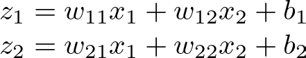
1: Input to Hidden Layer Let the initial weights from the input to the hidden layer be w11, w12, w21, w22, and the biases be b1, b2 for the two hidden neurons, respectively.
Given an input vector [x1, x2], the weighted sum for each neuron in the hidden layer is:
Hidden Layer Weighted Sum — Image by Author
Applying the ReLU activation function:
Hidden Layer ReLU Activation — Image by Author
1.2: Hidden Layer to Output:
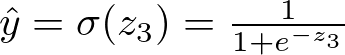
Let the weights from the hidden layer to the output neuron be w31, w32, and the bias be b3.
The weighted sum at the output neuron is:
Output Layer Weighted Sum — Image by Author
Applying the Sigmoid activation function for the output:
Output Layer Sigmoid Activation — Image by Author
Loss Calculation (Binary Cross-Entropy):
Cross-Entropy Formula — Image by Author
Backward Pass (Backpropagation): Now things get a bit more complex, as we need to calculate the gradient on the formulas we applied in the forward pass.
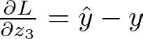
Output Layer Gradients Let’s start with the output layer. The derivative of the loss function for z3 is:
Output Layer Activation Gradient — Image by Author
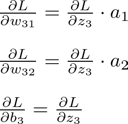
The gradients of the loss for weights and bias of the output layer:
Output Layer Gradient — Image by Author
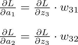
Hidden Layer Gradients The gradients of the loss for the hidden layer activations (chain rule applied):
Hidden Layer Activation Gradient — Image by Author
The gradients of the loss concerning weights and biases of the hidden layer:
Hidden Layer Gradient — Image by Author
These steps are then repeated until a criterion is met, such as a maximum number of epochs.
3.5: Improvements
While the basic idea of Gradient Descent is simple — take small steps in the direction that reduces error the most — several tweaks and improvements have been made to this method to enhance its efficiency and effectiveness.
Stochastic Gradient Descent (SGD) Stochastic Gradient Descent (SGD) takes the core idea of gradient descent but changes the approach by using just one training example at a time to calculate the gradient and update the weights. This method is similar to making decisions based on quick, individual observations rather than waiting to gather everyone’s opinion. It can make the learning process much faster because the model updates more frequently and with less computational burden.
Adam (Adaptive Moment Estimation) Adam, short for Adaptive Moment Estimation, is like the wise advisor to SGD’s youthful energy. It takes the concept of adjusting weights based on the data’s gradient but does so with a more sophisticated, personalized approach for each parameter in the model. Adam combines ideas from two other gradient descent improvements, AdaGrad and RMSProp, to adapt the learning rate for each weight in the network based on the first (mean) and second (uncentered variance) moments of the gradients.
Let’s finally recreate a neural network from scratch. For better readability, I will divide the code into 4 parts: NeuralNetwork class, Trainer class, and implementation.
You can find the whole code on this Jupyter Notebook. The notebook contains a fine-tuning bonus that will likely increase the performance of the Neural Network:
NeuralNetwork Class Let’s start with the NN class, which defines the architecture of our Neural Network:
import numpy as np
class NeuralNetwork: """ A simple neural network with one hidden layer.
Parameters: ----------- input_size: int The number of input features hidden_size: int The number of neurons in the hidden layer output_size: int The number of neurons in the output layer loss_func: str The loss function to use. Options are 'mse' for mean squared error, 'log_loss' for logistic loss, and 'categorical_crossentropy' for categorical crossentropy. """ def __init__(self, input_size, hidden_size, output_size, loss_func='mse'): self.input_size = input_size self.hidden_size = hidden_size self.output_size = output_size self.loss_func = loss_func
# track loss self.train_loss = [] self.test_loss = []
The __init__ method initializes a new instance of the NeuralNetwork class. It takes the size of the input layer (input_size), the hidden layer (hidden_size), and the output layer (output_size) as arguments, along with the type of loss function to use (loss_func), which defaults to mean squared error (‘mse’).
Inside this method, the network’s weights and biases are initialized. weights1 connects the input layer to the hidden layer, and weights2 connects the hidden layer to the output layer. The biases (bias1 and bias2) are initialized to zero arrays. This initialization uses random numbers for weights to break symmetry and zeros for biases as a starting point.
It also initializes two lists, train_loss and test_loss, to track the loss during the training and testing phases, respectively.
The forward method takes the input data X and passes it through the network. It calculates the weighted sums (z1, z2) and applies the activation function (sigmoid or softmax, depending on the loss function) to these sums to get the activations (a1, a2).
For the hidden layer, it always uses the sigmoid activation function. For the output layer, it uses softmax if the loss function is ‘categorical_crossentropy’ and sigmoid otherwise. The choice between sigmoid and softmax depends on the nature of the task (binary/multi-class classification).
This method returns the final output (a2) of the network, which can be used to make predictions.
Backpropagation (backward method)
def backward(self, X, y, learning_rate): # Perform backpropagation m = X.shape[0]
# Calculate gradients if self.loss_func == 'mse': self.dz2 = self.a2 - y elif self.loss_func == 'log_loss': self.dz2 = -(y/self.a2 - (1-y)/(1-self.a2)) elif self.loss_func == 'categorical_crossentropy': self.dz2 = self.a2 - y else: raise ValueError('Invalid loss function')
self.dw2 = (1 / m) * np.dot(self.a1.T, self.dz2) self.db2 = (1 / m) * np.sum(self.dz2, axis=0, keepdims=True) self.dz1 = np.dot(self.dz2, self.weights2.T) * self.sigmoid_derivative(self.a1) self.dw1 = (1 / m) * np.dot(X.T, self.dz1) self.db1 = (1 / m) * np.sum(self.dz1, axis=0, keepdims=True)
The backward method implements the backpropagation algorithm, which is used to update the weights and biases in the network based on the error between the predicted output and the actual output (y).
It calculates the gradients of the loss function for the weights and biases (dw2, db2, dw1, db1) using the chain rule. The gradients indicate how much the weights and biases need to be adjusted to minimize the error.
The learning rate (learning_rate) controls how big of a step is taken during the update. The method then updates the weights and biases by subtracting the product of the learning rate and their respective gradients.
Different gradient calculations are performed based on the chosen loss function, illustrating the flexibility of the network to adapt to various tasks.
sigmoid: This method implements the sigmoid activation function, which squashes the input values into a range between 0 and 1. It’s particularly useful for binary classification problems.
sigmoid_derivative: This computes the derivative of the sigmoid function, used during backpropagation to calculate gradients.
softmax: The softmax function is used for multi-class classification problems. It converts scores from the network into probabilities by taking the exponent of each output and then normalizing these values so that they sum up to 1.
Trainer Class The code below introduces a Trainer class designed to train a neural network model. It encapsulates everything needed to conduct training, including executing training cycles (epochs), calculating loss, and adjusting the model’s parameters through backpropagation based on the loss.
class Trainer: """ A class to train a neural network.
Parameters: ----------- model: NeuralNetwork The neural network model to train loss_func: str The loss function to use. Options are 'mse' for mean squared error, 'log_loss' for logistic loss, and 'categorical_crossentropy' for categorical crossentropy. """ def __init__(self, model, loss_func='mse'): self.model = model self.loss_func = loss_func self.train_loss = [] self.test_loss = []
def calculate_loss(self, y_true, y_pred): """ Calculate the loss.
Parameters: ----------- y_true: numpy array The true output y_pred: numpy array The predicted output
Returns: -------- float The loss """ if self.loss_func == 'mse': return np.mean((y_pred - y_true)**2) elif self.loss_func == 'log_loss': return -np.mean(y_true*np.log(y_pred) + (1-y_true)*np.log(1-y_pred)) elif self.loss_func == 'categorical_crossentropy': return -np.mean(y_true*np.log(y_pred)) else: raise ValueError('Invalid loss function')
Parameters: ----------- X_train: numpy array The training input data y_train: numpy array The training target output X_test: numpy array The test input data y_test: numpy array The test target output epochs: int The number of epochs to train the model learning_rate: float The learning rate """ for _ in range(epochs): self.model.forward(X_train) self.model.backward(X_train, y_train, learning_rate) train_loss = self.calculate_loss(y_train, self.model.a2) self.train_loss.append(train_loss)
The constructor takes a neural network model (model) and a loss function (loss_func) as inputs. The loss_func defaults to mean squared error (‘mse’) if not specified.
It initializes train_loss and test_loss lists to keep track of the loss values during the training and testing phases, allowing for monitoring of the model’s performance over time.
This method calculates the loss between the predicted outputs (y_pred) and the true outputs (y_true) using the specified loss function. This is crucial for evaluating how well the model is performing and for performing backpropagation.
The method supports three types of loss functions:
Mean Squared Error (‘mse’): Used for regression tasks, calculating the average of the squares of the differences between predicted and true values.
Logistic Loss (‘log_loss’): Suited for binary classification problems, computing the loss using the log-likelihood method.
Categorical Crossentropy (‘categorical_crossentropy’): Ideal for multi-class classification tasks, measuring the discrepancy between true labels and predictions.
If an invalid loss function is provided, it raises a ValueError.
The train method manages the training process over a specified number of epochs using the training (X_train, y_train) and testing datasets (X_test, y_test). It also takes a learning_rate parameter that influences the step size in the parameter update during backpropagation.
For each epoch (training cycle), the method performs the following steps:
Forward Pass on Training Data: It uses the model’s forward method to compute the predicted outputs for the training data.
Backward Pass (Parameter Update): It applies the model’s backward method using the training data and labels (y_train) along with the learning_rate to update the model’s weights and biases based on the gradients calculated from the loss.
Calculate Training Loss: The training loss is calculated using the calculate_loss method with the training labels and the predictions. This loss is then appended to the train_loss list for monitoring.
Forward Pass on Testing Data: Similarly, the method computes predictions for the testing data to evaluate the model’s performance on unseen data.
Calculate Testing Loss: It calculates the testing loss using the testing labels and predictions, appending this loss to the test_loss list.
Implementation In this section, I will outline a complete process for loading a dataset, preparing it for training, and using it to train a neural network for a classification task. The process involves data preprocessing, model creation, training, and evaluation.
# Convert y_test from one-hot encoding to labels y_test_labels = np.argmax(y_test, axis=1)
# Evaluate the performance of the neural network predictions = np.argmax(nn.forward(X_test), axis=1) accuracy = np.mean(predictions == y_test_labels) print(f"Accuracy: {accuracy:.2%}")
Let’s walk through each step:
Load the Dataset
# Load the digits dataset
digits = load_digits()
Digits Dataset First 10 Images — Image by Author
The dataset used here is the digits dataset, which is commonly used for classification tasks involving recognizing handwritten digits.
Preprocess the Dataset
# Preprocess the dataset
scaler = MinMaxScaler()
X = scaler.fit_transform(digits.data)
y = digits.target
The features of the dataset are scaled to a range between 0 and 1 using the MinMaxScaler. This is a common preprocessing step to ensure that all input features have the same scale, which can help the neural network learn more effectively.
The scaled features are stored in X, and the target labels (which digit each image represents) are stored in y.
Since this is a classification task with multiple classes, the target labels are one-hot encoded using OneHotEncoder. One-hot encoding transforms the categorical target data into a format that’s easier for neural networks to understand and work with, especially for classification tasks.
Split the Dataset
# Split the dataset into training and testing sets
X_train, X_test, y_train, y_test = train_test_split(X, y_onehot, test_size=0.2, random_state=42)
The dataset is split into training and testing sets using train_test_split, with 80% of the data used for training and 20% for testing. This split allows for training the model on one portion of the data and then evaluating its performance on a separate, unseen portion to check how well it generalizes.
Create an Instance of the NeuralNetwork Class
# Create an instance of the NeuralNetwork class
input_size = X.shape[1]
hidden_size = 64
output_size = len(np.unique(y))
loss_func = 'categorical_crossentropy'
epochs = 1000
learning_rate = 0.1

nn = NeuralNetwork(input_size, hidden_size, output_size, loss_func)
A neural network instance is created with specified input size (the number of features), hidden size (the number of neurons in the hidden layer), output size (the number of unique labels), and the loss function to use. The input size matches the number of features, the output size matches the number of unique target classes, and a hidden layer size is chosen.
An instance of the Trainer class is created with the neural network and loss function. The train method is then called with the training and testing datasets, along with the number of epochs and the learning rate specified. This process iteratively adjusts the neural network’s weights and biases to minimize the loss function, using the training data for learning and the testing data for validation.
Evaluate the Performance
# Convert y_test from one-hot encoding to labels
y_test_labels = np.argmax(y_test, axis=1)

# Evaluate the performance of the neural network
predictions = np.argmax(nn.forward(X_test), axis=1)
accuracy = np.mean(predictions == y_test_labels)
print(f"Accuracy: {accuracy:.2%}")
After training, the model’s performance is evaluated on the test set. Since the targets were one-hot encoded, np.argmax is used to convert the one-hot encoded predictions back to label form. The accuracy of the model is calculated by comparing these predicted labels against the actual labels (y_test_labels) and then printed out.
Now, this code lacks a few activation functions we talked about, improvements such as SGD or Adam Optimizer, and more. I leave this to you to take and make this code your own, by filling the gaps with your code. In this way, you will truly master Neural Networks.
4.2: Utilizing Libraries for Neural Network Implementation (TensorFlow)
Well, that was a lot! Luckily for us, we don’t need to write such a long code every time we want to work with NNs. We can leverage libraries such as Tensorflow and PyTorch which will create Deep Learning models for us with minimum code. In this example, we will create and explain a TensorFlow version of training a neural network on the digits dataset, similar to the process described previously.
As before let’s first import the required libraries, and the dataset and let’s preprocess it, in the same fashion we did before.
import tensorflow as tf from sklearn.datasets import load_digits from sklearn.model_selection import train_test_split from sklearn.preprocessing import MinMaxScaler, OneHotEncoder
# Load the digits dataset digits = load_digits()
# Scale the features to a range between 0 and 1 scaler = MinMaxScaler() X_scaled = scaler.fit_transform(digits.data)
# Split the dataset into training and testing sets X_train, X_test, y_train, y_test = train_test_split(X_scaled, y_onehot, test_size=0.2, random_state=42)
Secondly, let’s build the NN:
# Define the model architecture
model = tf.keras.models.Sequential([
    tf.keras.layers.Dense(64, activation='relu', input_shape=(X_train.shape[1],)),
    tf.keras.layers.Dense(len(np.unique(digits.target)), activation='softmax')
])
Here, a Sequential model is created, indicating a linear stack of layers.
The first layer is a densely-connected layer with 64 units (neurons) and ReLU activation. It expects input from the shape (X_train.shape[1],), which matches the number of features in the dataset.
The output layer has several units equal to the number of unique target classes and uses the softmax activation function to output probabilities for each class.
# Compile the model
model.compile(optimizer='adam',
              loss='categorical_crossentropy',
              metrics=['accuracy'])
The model is compiled with the Adam optimizer and categorical cross-entropy as the loss function, suitable for multi-class classification tasks. Accuracy is specified as a metric for evaluation.
Lastly, let’s train and evaluate the performance of our NN:
# Train the model
history = model.fit(X_train, y_train, epochs=1000, validation_data=(X_test, y_test), verbose=2)

# Evaluate the model on the test set
test_loss, test_accuracy = model.evaluate(X_test, y_test, verbose=2)
print(f"Test accuracy: {test_accuracy:.2%}")
The model is trained using the fit method with 1000 epochs, and the testing set is used as validation data. verbose=2 indicates that one line per epoch will be printed for logging.
Finally, the model’s performance is evaluated on the test set using the evaluate method, and the test accuracy is printed.
5: Challenges
5.1: Overcoming Overfitting
Overfitting is like when a neural network becomes a bit too obsessed with its training data, picking up on all the tiny details and noise, to the point where it struggles to handle new, unseen data. It’s like studying so hard for your exams by memorizing the textbook word for word but then not being able to apply what you’ve learned to any question that’s phrased differently. This problem can hold back a model’s ability to perform well in real-world situations, where being able to generalize or apply what it’s learned to new scenarios, is key. Luckily, there are several clever techniques to help prevent or lessen overfitting, making our models more versatile and ready for the real world. Let’s take a look at a few of them, but don’t worry about mastering all of them now as I will cover anti-overfitting techniques in a separate article.
Dropout: This is like randomly turning off some of the neurons in the network during training. It stops the neurons from getting too dependent on each other, forcing the network to learn more robust features that aren’t just relying on a specific set of neurons to make predictions.
Early Stopping This involves watching how the model does on a validation set (a separate chunk of data) as it’s training. If the model starts doing worse on this set, it’s a sign that it’s beginning to overfit, and it’s time to stop training.
Using a Validation Set Dividing your data into three sets — training, validation, and test — helps keep an eye on overfitting. The validation set is for tuning the model and picking the best version, while the test set gives you a fair assessment of how well the model is doing.
Simplifying The Model Sometimes, less is more. If a model is too complex, it might start picking up noise from the training data. By choosing a simpler model or dialing back on the number of layers, we can reduce the risk of overfitting.
As you experiment with NN, you will see that fine-tuning and tackling overfitting will play a pivotal role in NN’s performance. Making sure you master anti-overfitting techniques is a must for a successful data scientist. Because of its importance, I will dedicate an entire article to these techniques to make sure you can fine-tune the best NNs and guarantee an optimal performance for your projects.
6: Conclusion
Diving into the world of neural networks opens our eyes to the incredible potential these models hold within the realm of artificial intelligence. Starting with the basics, like how neural networks use weighted sums and activation functions to process information, we’ve seen how techniques like backpropagation and gradient descent empower them to learn from data. Especially in areas like image recognition, we’ve witnessed firsthand how neural networks are solving complex challenges and pushing technology forward.
Looking ahead, it’s clear we are only at the beginning of a long journey called “Deep Learning”. In the next articles, we will talk about more advanced deep learning architectures, fine-tuning methods, and much more!
Bibliography
Goodfellow, Ian, Yoshua Bengio, and Aaron Courville. “Deep Learning.” MIT Press, 2016. This comprehensive textbook provides an extensive overview of deep learning, covering the mathematical underpinnings and practical aspects of neural networks.
LeCun, Yann, Yoshua Bengio, and Geoffrey Hinton. “Deep learning.” Nature 521, no. 7553 (2015): 436–444. A landmark paper by pioneers in the field, summarizing the key concepts and achievements in deep learning and neural networks.
You made it to the end. Congrats! I hope you enjoyed this article, if so consider leaving a like and following me, as I will regularly post similar articles. My goal is to recreate all the most popular algorithms from scratch and make machine learning accessible to everyone.
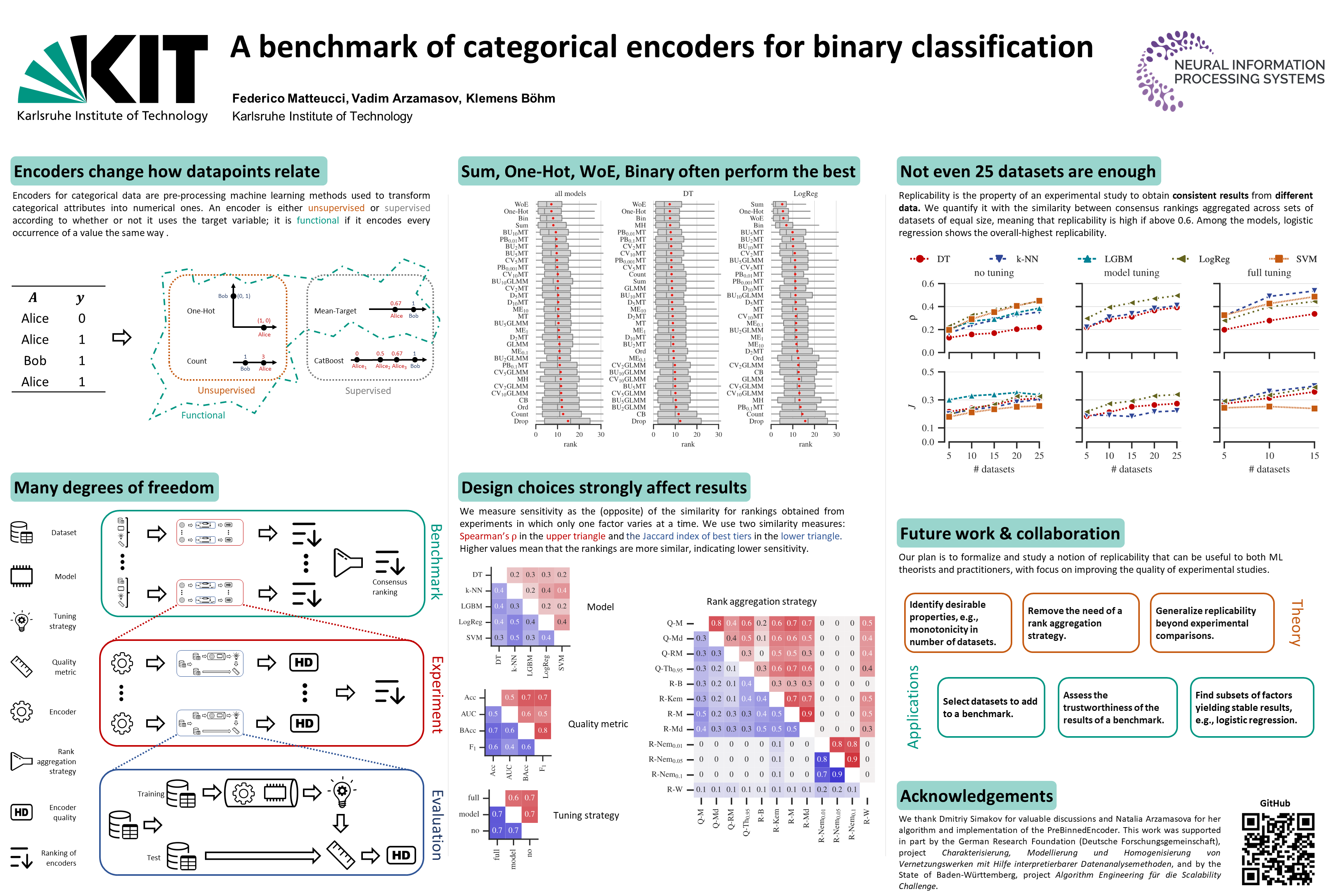
A large share of datasets contain categorical features. For example, out of 665 datasets on the UC Irvine Machine Learning Repository [1], 42 are fully categorical and 366 are reported as mixed. However, distance-based ML models require features in a numerical format. Categorical encoders replace the categories in such features with real numbers.
A variety of categorical encoders exist, but there have been few attempts to compare them on many datasets, with various ML models, and in different pipelines. This article is about one of the latest benchmarks of encoders from our recent publication [2] (poster, code on GitHub). In this story, I focus on the content that complements the publication and is of practical importance. In particular, beyond the summary of our benchmark results, I will:
Provide a list of 55 categorical encoders and the links to find their explanations and implementations for most of them.
Explain that you can also use our code as a supplement to the Category Encoderspython module for the encoders not yet implemented there.
Categorize the encoders into families so that you do not have to remember each individual encoder, but instead have an idea of how to build a member of each family.
Explain how you can reuse the code from [2] and detailed benchmark data to include your encoder, dataset, or ML models in the comparison without having to re-run the existing experiments. Depending on the scope of your experiments and your computational resources, this can save you weeks of computation.
Why another benchmark?
There are already several scientific studies comparing categorical encoders [3–12] and at least one categorical encoder benchmark on TDS [13]. The study [2] that I will present here differs mainly in scope: We compared representative encoders in different configurations from a variety of encoder families. We experimented with 5 ML models (decision tree, kNN, SVM, logistic regression, LGBM), 4 quality metrics (AUC, accuracy, balanced accuracy, F1-score), 3 tuning strategies (which I will describe shortly), 50 datasets, and 32 encoder configurations.
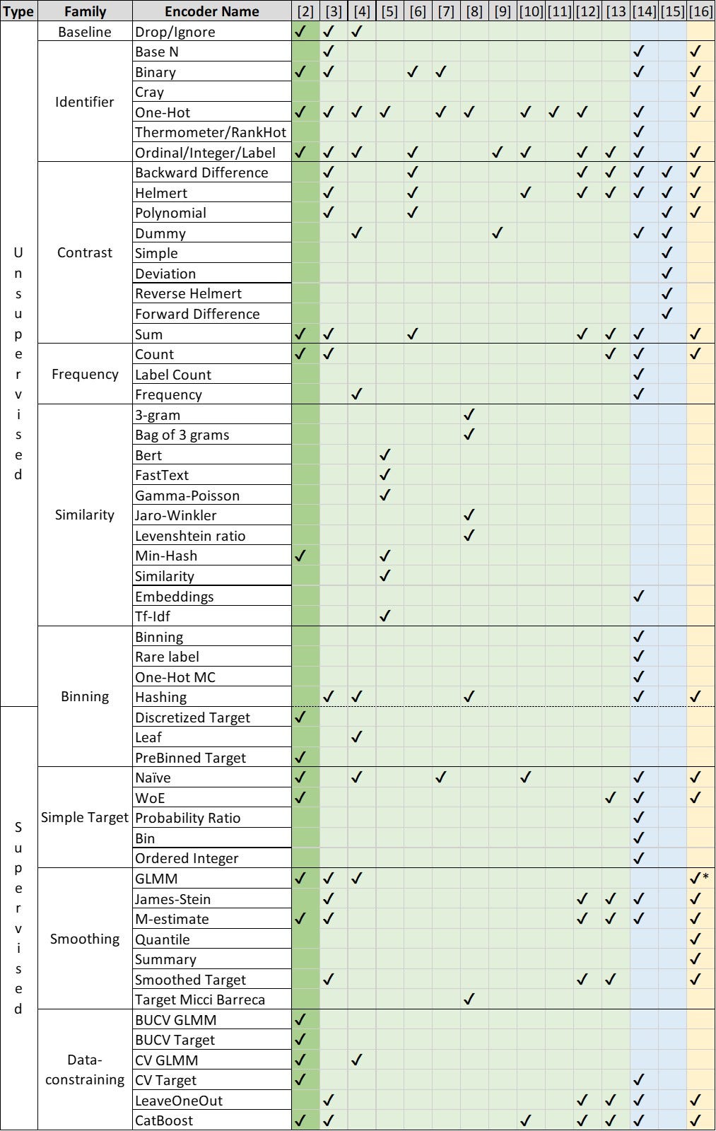
The following table shows the encoders covered in our benchmark (the dark green column) and in other experimental comparisons (the light green columns). The blue columns show the encoders described in two additional sources: on Medium [14] and in the article dedicated to contrast encoders [15]. The last yellow column shows the encoders covered by the Category Encoders module [16]. Note that the code from [2] implements some encoders — from the similarity, binning, and data constraining families — that are not part of the Category Encoders module. In addition, we have found that the interface to the GLMM encoder implemented in R and used in [2] is much faster than the GLMM encoder from Category Encoders. Therefore, you may find our code useful for these implementations.
Table 1. Encoder families and their coverage by various resources. Author owns copyright
Table 1 already contains a number of encoders, and the list is by no means exhaustive. To navigate the encoder landscape, it is therefore useful to classify encoders in order to understand the principles of encoder design, rather than to memorize a large number of individual encoders.
Families of encoders
In the following, we consider a categorical feature of length n with cardinality k. At the top level, categorical encoders are supervised or unsupervised.
1. Unsupervised encoders do not include the target variable in the encoding process.
1.1. Identifier encoders transform categorical variables using a bijective function, i.e., they assign each category a unique numeric value or a unique combination of numeric values. They create from 1 up to k new features. For example, One-Hot encoder creates k features, label or ordinal encoders create a single new feature, Base N encoders create ⌈log(k)⌉ new features, where the logarithm is of base N.
These encoders are useful for categorical variables that denote unique identifiers, such as product codes or zip codes. Typically, with the exception of ordinal encoder, identifier encoders do not assume that any inherent order in the categories conveys meaningful information for analysis, and thus ignore any such order during the encoding process.
1.2. Contrast encoders transform categorical variables by assigning numerical values based on comparisons between categories. Typically, a set of k-1 new features represents a categorical variable with k categories. Unlike identifier encoders, these encoders are specifically designed to explore the relationships between different levels of a categorical variable in a regression analysis.
To create a contrast encoder, one has a choice of different coding schemes [15]. Each contrasts a category with other categories in a particular way to test a related hypothesis about the data. For example, Helmert coding contrasts each level with the mean of subsequent levels, while sum coding contrasts each level with the overall mean.
1.3. Frequency encoders replace the categories of a categorical variable with corresponding values that are a function of the frequency of those categories in the data set. Unlike identifier or contrast encoders, frequency encoders do not guarantee to assign unique identifiers and create a single new feature. They provide a numerical representation of occurrence rates, which can be particularly useful when an ML model benefits from understanding the commonality of category values. All three frequency encoders in Table 1 are monotonically increasing functions of frequency. However, this is not a necessary condition for defining this group.
1.4. Similarity encoders [5, 8, 18] transform categorical data into numerical form by applying similarity or distance metrics that capture similarities between different categories.
One group of similarity encoders [8, 18] is based on a morphological comparison between two categories treated as strings. Examples of similarity metrics are Levenshtein’s ratio, Jaro-Winkler similarity, or N-gram similarity. The categorical variable is then encoded as a vector, where each dimension corresponds to a pairwise comparison of a reference category with all categories, and the value represents the computed similarity score (similar to constructing a variance-covariance matrix). Encoders of this group typically create k new features. This encoding is particularly useful for handling “dirty” categorical datasets that may contain typos and redundancies [18]. One can think of One-Hot encoding as a special case of similarity encoding, where the similarity measure can take only two values, 0 or 1.
Another group of similarity encoders [5], including, e.g. Embeddings, Min-Hash, or Gamma-Poisson matrix factorization, is designed for high cardinality categories (k>>1). They project categorical features into a lower dimensional space. This group is thus similar to binning encoders, which are also particularly useful for large k but do not aim to preserve the morphological similarity of categories.
2. Supervised encoders use information about the target variable. For regression or binary classification tasks, they typically create a single new feature for each categorical one.
2.1.Simple target encoders capture the relationship between the categorical characteristic and the target. Constructing a simple target encoder involves calculating a statistic based on the target variable for each level of the categorical variable. Common statistics include the mean, median, or probability ratios of the target variable conditional on each category.
The procedure is as follows:
For each category level, group the data by the categorical variable.
Within each group, compute the desired statistic of interest.
For each instance in the data, replace the original categorical value with the corresponding statistic.
Simple target encoding runs the risk of overfitting, especially for small data sets and categories with very few observations. Techniques such as smoothing (regularization) and cross-validation, which we describe shortly, can help mitigate this risk.
2.2. Smoothing encoders are generalizations of simple target encoders that introduce a smoothing parameter. The purpose of this smoothing parameter is to prevent overfitting and to improve the generalization of the encoder to new data, especially when there are categories with a small number of observations. A common formula for the smoothed value is
where m is the number of times the category occurs in the data set. It may slightly vary, see [13]. By adjusting the smoothing parameter, you can control the balance between the category statistic and the overall statistic. A larger smoothing parameter makes the encoding less sensitive to the category-specific target statistic. Setting the smoothing parameter to zero in the above formula results in a simple target encoding.
2.3. Data-constraining encoders use information from a subset of rows in a data set. An example of a data-constraining coder is the leave-one-out coder, which, for a given categorical value, calculates the statistic of the target variable for all other instances in which the category occurs, excluding the current instance. This approach ensures that the encoded value for a given data set does not include its own target value.
Data-constraining strategies help create encodings that are more representative of the true relationships in the unseen data and less prone to overfitting. The number of unique values in the encoded column may exceed the cardinality of the original categorical column k. One can also introduce smoothing into data-constraining encodings.
3. Binning encoders can be both supervised and unsupervised. Often, their work can be divided into two steps. The first step creates an auxiliary categorical feature by sorting the original categories into bins. The second step applies an encoder from one of the other groups discussed above to this auxiliary feature. Both steps can be either unsupervised or supervised independently of each other. For example, in the first step, you can form the bins by grouping rare categories together (unsupervised, e.g., One-Hot MC encoder); alternatively, you can apply a simple target encoder and group the categories with close encoded values together (supervised, e.g., Discretized Target encoder).
Some binning encoders, e.g. Hashing, do not have this two-stage structure. The number of new features created by binning encoders is usually <k.
Tuning strategies
Before proceeding with the results, I will briefly summarize the tuning strategies from our benchmark. This is important to understand the scope of the following figures and to reuse the data and code from our benchmark. The three tuning strategies are
No tuning:
Encode the categorical columns of the training data;
Train an ML model with its default hyperparameters.
Model tuning:
Encode the categorical columns of the training data;
Divide the training data into folds;
Optimize the hyperparameters of an ML model using cross-validation.
Full tuning:
Split training data into folds;
Encode each training fold separately (in case of data constraining encoder family, each fold is further split into the nested folds);
Optimize the hyperparameters of an ML model with cross-validation.
Results
I will name the winning encoders from our experiments, point out which tuning strategy performed best and should be part of your ML pipeline, and present the runtimes for various encoders.
Ranking
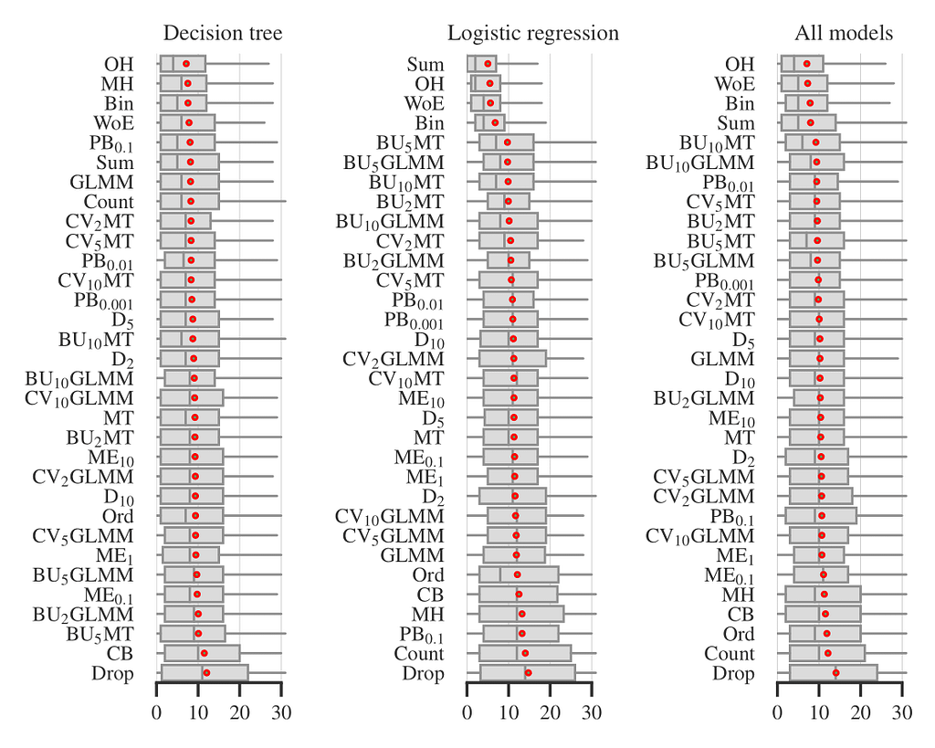
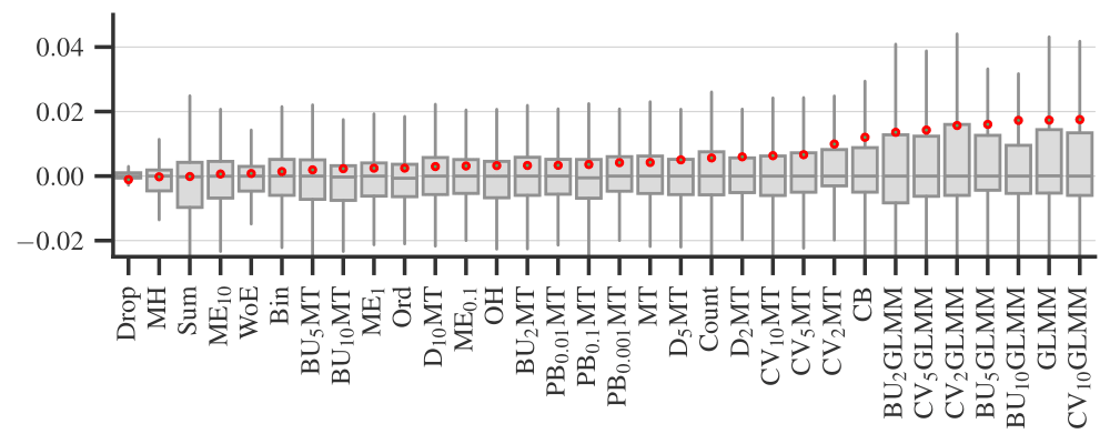
Figure 1. Performance of encoders in all experiments. Author owns copyright
In Figure 1, the boxplots show the distribution of encoder ranks across all datasets, quality metrics, and tuning strategies. That is, each boxplot includes ~50×4×3=600 experiments for individual models and ~50×4×3×5=3000 experiments for all models, excluding the small fraction of experiments that timed out or failed for other reasons. We observed that four encoders: One-Hot, Binary (‘Bin’ on the plot), Sum, and Weight of Evidence are consistently among the best performing. For logistic regression, the difference of these four from the rest is statistically significant. This result is somewhat surprising since many previous studies (see [13, 14]) have reported drawbacks of unsupervised encoders, especially One-Hot. The exact meanings of all other encoder abbreviations on Figure 1 are not important for the rest, but you can find them in [2].
Tuning strategy
Figure 2. Performance gain of full tuning over no tuning. Author owns copyrightFigure 3. Performance gain of full tuning over model tuning. Author owns copyright
Figure 2 plots the performance difference between full and no tuning strategies (as I described above) for each categorical encoder. Each covers the experiments with different datasets, ML models, and performance metrics. Figure 3 is a similar plot comparing full and model tuning strategies. Note that these plots do not include some of the ML models and datasets because we limited the computational complexity. See [2] for details and more plots.
Based on these results, I would generally recommend sticking to the full tuning strategy, i.e., encoding data for each fold separately when optimizing the hyperparameters of an ML model; this is especially important for data constraining encoders.
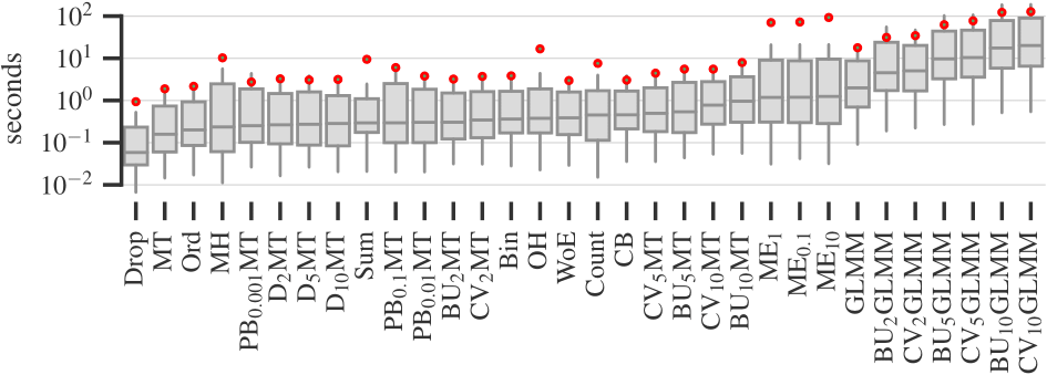
Runtime
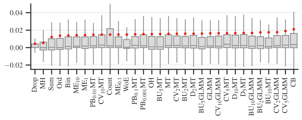
Figure 4. Runtime of encoders. Author owns copyright
Finally, Figure 4 plots the times required to encode data sets on a logarithmic scale. Simple target and binning encoders are the fastest, while smoothing and data constraining encoders are the slowest. The four best performing encoders — One-Hot, Binary (‘Bin’ on the plot), Sum, and Weight of Evidence — take a reasonable amount of time to process data.
Reusing the code and the results
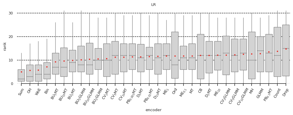
A nice feature of our benchmark is that you can easily extend it to test your approach to categorical encoding and put it in the context of existing experimental results. For example, you may want to test the encoders from Table 1 that are not part of our benchmark, or you may want to test your custom composite encoder like if n/k>a then One-Hot MC else One-Hot where k is the feature cardinality and n is the size of the dataset, as before. We explain the process on GitHub and share the demonstration of how to do this in the kaggle notebook [17]. Below is a short summary of [17].
For illustrative purposes, we limited the example to a logistic regression model without hyperparameter tuning. The corresponding results of our benchmark are shown in Figure 5 below.
Figure 5. Encoder ranks for logistic regression with no tuning strategy. Author owns copyright
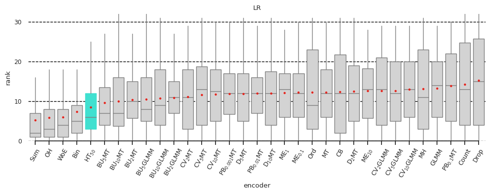
Now suppose that Yury Kashnitsky, who kindly provided feedback on our paper, wonders whether the hashing encoder is competitive with the encoders we evaluated. In [17], we show how to perform the missing experiments and find that the hashing encoder performs reasonably well with our choice of its hyperparameter, as Figure 6 shows.
I summarized our benchmark of categorical encoders and explained how you can benefit from our shared artifacts. You may have learned:
Categorical encoders, as ML models, can be supervised or unsupervised.
I presented eight families of encoders. Some encoders preserve the cardinality of categorical features, others can reduce it (often the case for binning, but also for some other encoders, e.g., Naive Target) or increase it (data constraining).
One-Hot, Binary, Sum, and Weight of Evidence encoders performed best on average in our experiments, especially with logistic regression.
See the kaggle notebook [17] for a demo of how to add the desired encoders to the benchmark and plot the results; the necessary code is available on GitHub.
Acknowledgements
This story would not exist if Federico Matteucci, my colleague and first author in [2], had not written the code for the benchmark and for the kaggle notebook [17].
We use cookies on our website to give you the most relevant experience by remembering your preferences and repeat visits. By clicking “Accept”, you consent to the use of ALL the cookies.
This website uses cookies to improve your experience while you navigate through the website. Out of these, the cookies that are categorized as necessary are stored on your browser as they are essential for the working of basic functionalities of the website. We also use third-party cookies that help us analyze and understand how you use this website. These cookies will be stored in your browser only with your consent. You also have the option to opt-out of these cookies. But opting out of some of these cookies may affect your browsing experience.
Necessary cookies are absolutely essential for the website to function properly. These cookies ensure basic functionalities and security features of the website, anonymously.
Cookie
Duration
Description
cookielawinfo-checkbox-analytics
11 months
This cookie is set by GDPR Cookie Consent plugin. The cookie is used to store the user consent for the cookies in the category "Analytics".
cookielawinfo-checkbox-functional
11 months
The cookie is set by GDPR cookie consent to record the user consent for the cookies in the category "Functional".
cookielawinfo-checkbox-necessary
11 months
This cookie is set by GDPR Cookie Consent plugin. The cookies is used to store the user consent for the cookies in the category "Necessary".
cookielawinfo-checkbox-others
11 months
This cookie is set by GDPR Cookie Consent plugin. The cookie is used to store the user consent for the cookies in the category "Other.
cookielawinfo-checkbox-performance
11 months
This cookie is set by GDPR Cookie Consent plugin. The cookie is used to store the user consent for the cookies in the category "Performance".
viewed_cookie_policy
11 months
The cookie is set by the GDPR Cookie Consent plugin and is used to store whether or not user has consented to the use of cookies. It does not store any personal data.
Functional cookies help to perform certain functionalities like sharing the content of the website on social media platforms, collect feedbacks, and other third-party features.
Performance cookies are used to understand and analyze the key performance indexes of the website which helps in delivering a better user experience for the visitors.
Analytical cookies are used to understand how visitors interact with the website. These cookies help provide information on metrics the number of visitors, bounce rate, traffic source, etc.
Advertisement cookies are used to provide visitors with relevant ads and marketing campaigns. These cookies track visitors across websites and collect information to provide customized ads.


