This is how to make your pandas code human readable & bulletproof.
Scripting around a pandas DataFrame can turn into an awkward pile of (not-so-)good old spaghetti code. Me and my colleagues use this package a lot and while we try to stick to good programming practices, like splitting code in modules and unit testing, sometimes we still get in the way of one another by producing confusing code.
I have gathered some tips and pitfalls to avoid in order to make pandas code clean and infallible. Hopefully you’ll find them useful too. We’ll get some help from Robert C. Martin’s classic “Clean code” specifically for the context of the pandas package. TL;DR at the end.
Dont’s
Let’s begin by observing some faulty patterns inspired by real life. Later on, we’ll try to rephrase that code in order to favor readability and control.
Mutability
Pandas DataFrames are value-mutable [2, 3] objects. Whenever you alter a mutable object, it affects the exact same instance that you originally created and its physical location in memory remains unchanged. In contrast, when you modify an immutable object (eg. a string), Python goes to create a whole new object at a new memory location and swaps the reference for the new one.
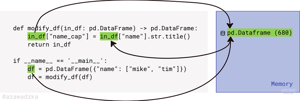
This is the crucial point: in Python, objects get passed to the function by assignment[4, 5]. See the graph: the value of df has been assigned to variable in_df when it was passed to the function as an argument. Both the original df and the in_df inside the function point to the same memory location (numeric value in parentheses), even if they go by different variable names. During the modification of its attributes, the location of the mutable object remains unchanged. Now all other scopes can see the changes too — they reach to the same memory location.
Modification of a mutable object in Python memory.
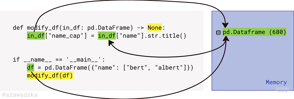
Actually, since we have modified the original instance, it’s redundant to return the DataFrame and assign it to the variable. This code has the exact same effect:
Modification of a mutable object in Python memory, redundant assignment removed.
Heads-up: the function now returns None, so be careful not to overwrite the df with None if you do perform the assignment: df = modify_df(df).
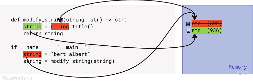
In contrast, if the object is immutable, it will change the memory location throughout the modification just like in the example below. Since the red string cannot be modified (strings are immutable), the green string is created on top of the old one, but as a brand new object, claiming a new location in memory. The returned string is not the same string, whereas the returned DataFrame was the exact same DataFrame.
Modification of an immutable object in Python memory.
The point is, mutating DataFrames inside functions has a global effect. If you don’t keep that in mind, you may:
accidentally modify or remove part of your data, thinking that the action is only taking place inside the function scope — it is not,
lose control over what is added to your DataFrame and when it’s added, for example in nested function calls.
Output arguments
We’ll fix that problem later, but here is another don’t before we pass to do’s
The design from the previous section is actually an anti-pattern called output argument [1 p.45]. Typically, inputs of a function will be used to create an output value. If the sole point of passing an argument to a function is to modify it, so that the input argument changes its state, then it’s challenging our intuitions. Such behavior is called side effect [1 p.44] of a function and those should be well documented and minimized because they force the programmer to remember the things that go in the background, therefore making the script error-prone.
When we read a function, we are used to the idea of information going in to the function through arguments and out through the return value. We don’t usually expect information to be going out through the arguments. [1 p.41]
Things get even worse if the function has a double responsibility: to modify the input and to return an output. Consider this function:
It does return a value as you would expect, but it also permanently modifies the original DataFrame. The side effect takes you by surprise – nothing in the function signature indicated that our input data was going to be affected. In the next step, we’ll see how to avoid this kind of design.
Do’s
Reduce modifications
To eliminate the side effect, in the code below we have created a new temporary variable instead of modifying the original DataFrame. The notation lengths: pd.Series indicates the datatype of the variable.
This function design is better in that it encapsulates the intermediate state instead of producing a side effect.
Another heads-up: please be mindful of the differences between deep and shallow copy[6] of elements from the DataFrame. In the example above we have modified each element of the original df[“name”] Series, so the old DataFrame and the new variable have no shared elements. However, if you directly assign one of the original columns to a new variable, the underlying elements still have the same references in memory. See the examples:
df = pd.DataFrame({"name": ["bert", "albert"]})

series = df["name"]     # shallow copy
series[0] = "roberta"   # <-- this changes the original DataFrame

series = df["name"].copy(deep=True)
series[0] = "roberta"   # <-- this does not change the original DataFrame

series = df["name"].str.title()  # not a copy whatsoever
series[0] = "roberta"   # <-- this does not change the original DataFrame
You can print out the DataFrame after each step to observe the effect. Remember that creating a deep copy will allocate new memory, so it’s good to reflect whether your script needs to be memory-efficient.
Group similar operations
Maybe for whatever reason you want to store the result of that length computation. It’s still not a good idea to append it to the DataFrame inside the function because of the side effect breach as well as the accumulation of multiple responsibilities inside a single function.
I like the One Level of Abstraction per Function rule that says:
We need to make sure that the statements within our function are all at the same level of abstraction.
Mixing levels of abstraction within a function is always confusing. Readers may not be able to tell whether a particular expression is an essential concept or a detail. [1 p.36]
Also let’s employ the Single responsibility principle [1 p.138] from OOP, even though we’re not focusing on object-oriented code right now.
Why not prepare your data beforehand? Let’s split data preparation and the actual computation in separate functions.:
The individual task of creating the name_len column has been outsourced to another function. It does not modify the original DataFrame and it performs one task at a time. Later we retrieve the max element by passing the new column to another dedicated function. Notice how the aggregating function is generic for Collections.
Let’s brush the code up with the following steps:
We could use concat function and extract it to a separate function called prepare_data, which would group all data preparation steps in a single place,
We could also make use of the apply method and work on individual texts instead of Series of texts,
Let’s remember to use shallow vs. deep copy, depending on whether the original data should or should not be modified:
The way we have split the code really makes it easy to go back to the script later, take the entire function and reuse it in another script. We like that!
There is one more thing we can do to increase the level of reusability: pass column names as parameters to functions. The refactoring is going a little bit over the top, but sometimes it pays for the sake of flexibility or reusability.
Did you ever figure out that your preprocessing was faulty after weeks of experiments on the preprocessed dataset? No? Lucky you. I actually had to repeat a batch of experiments because of broken annotations, which could have been avoided if I had tested just a couple of basic functions.
Important scripts should be tested [1 p.121, 7]. Even if the script is just a helper, I now try to test at least the crucial, most low-level functions. Let’s revisit the steps that we made from the start:
1. I am not happy to even think of testing this, it’s very redundant and we have paved over the side effect. It also tests a bunch of different features: the computation of name length and the aggregation of result for the max element. Plus it fails, did you see that coming?
2. This is much better — we have focused on one single task, so the test is simpler. We also don’t have to fixate on column names like we did before. However, I think that the format of the data gets in the way of verifying the correctness of the computation.
3. Here we have cleaned up the desk. We test the computation function inside out, leaving the pandas overlay behind. It’s easier to come up with edge cases when you focus on one thing at a time. I figured out that I’d like to test for None values that may appear in the DataFrame and I eventually had to improve my function for that test to pass. A bug caught!
def compute_length(word: Optional[str]) -> int: return len(word) if word else 0
One additional benefit of unit testing that I never forget to mention is that it is a way of documenting your code, as someone who doesn’t know it (like you from the future) can easily figure out the inputs and expected outputs, including edge cases, just by looking at the tests. Double gain!
Conclusion
These are some tricks I found useful while coding and reviewing other people’s code. I’m far from telling you that one or another way of coding is the only correct one — you take what you want from it, you decide whether you need a quick scratch or a highly polished and tested codebase. I hope this thought piece helps you structure your scripts so that you’re happier with them and more confident about their infallibility.
If you liked this article, I would love to know about it. Happy coding!
TL;DR
There’s no one and only correct way of coding, but here are some inspirations for scripting with pandas:
Dont’s:
– don’t mutate your DataFrame too much inside functions, because you may lose control over what and where gets appended/removed from it,
– don’t write methods that mutate a DataFrame and return nothing because that’s confusing.
Do’s:
– create new objects instead of modifying the source DataFrame and remember to make a deep copy when needed,
– perform only similar-level operations inside a single function,
– design functions for flexibility and reusability,
– test your functions because this helps you design cleaner code, secure against bugs and edge cases and document it for free.
References
[1] Robert C. Martin, Clean code A Handbook of Agile Software Craftsmanship (2009), Pearson Education, Inc.
For many researchers, outliers are rogue waves that can dramatically alter the course of the analysis or “confound” some expected effects. I prefer to use the term “extreme observations” and leave the term outlier for observations that are not truly part of the population being studied. For example, in my field (brain ischemia research), an outlier is an animal that does not have ischemia (when it should have), while extreme observations are animals with small or large ischemias that are very different from the others.
Traditional (frequentist) statistical models are built on the strong foundation of Gaussian distributions. This has a significant limitation: an inherent assumption that all data points will cluster around a central mean in a predictable pattern (based on the central limit theorem). This may be true in Plato’s world of ideas, but we, scientists in the biomedical field, are aware it’s challenging to rely on this assumption given the limited sampling (number of animals) we have available to make observations.
Gaussian distributions are very sensitive to extreme observations, and their use leads scientists to believe that eliminating extreme observations is the best way to get “clearer” or “cleaner” results (whatever that means). As I once commented in an article as reviewer 2, “The problem is not the extreme observations that may “hide” your effects, but the fact that you are using a statistical model that (I believe) is inappropriate for your purposes”.
It should be noted that no statistical model is the “right” or “appropriate” one, but we can estimate that, given the data, there are certain statistical models that are more likely to generate the observed data (generative models) than others.
Fortunately, nothing forces us to be bound by the assumptions of the Gaussian models, right? We have other options, such as the Student’s t-distribution (1). I see it as a more adaptable vessel to navigate the turbulent seas of real-world biomedical data. The Student’s t-distribution provides a robust alternative to acknowledge that our data may be populated by extreme observations that are normal biological responses that we can expect in any context. There may be patients or animals that don’t respond or overreact to treatment, and it is valuable that our modeling approach recognizes these responses as part of the spectrum. Therefore, this tutorial explores the modeling strategies using Student’s t-distributions through the lens of the brms package for R (2)—a powerful ally for Bayesian modeling
What’s behind a student’s t-distribution?
A Student’s t-distribution is nothing more than a Gaussian distribution with heavier tails. In other words, we can say that the Gaussian distribution is a special case of the Student’s t-distribution. The Gaussian distribution is defined by the mean (μ) and the standard deviation (σ). The Student t distribution, on the other hand, adds an additional parameter, the degrees of freedom (df), which controls the “thickness” of the distribution. This parameter assigns greater probability to events further from the mean. This feature is particularly useful for small sample sizes, such as in biomedicine, where the assumption of normality is questionable. Note that as the degrees of freedom increase, the Student t-distribution approaches the Gaussian distribution. We can visualize this using density plots:
# Create a data frame for plotting df <- data.frame(x, y_gaussian, y_t3, y_t10, y_t30)
# Plot the distributions ggplot(df, aes(x)) + geom_line(aes(y = y_gaussian, color = "Gaussian")) + geom_line(aes(y = y_t3, color = "t, df=3")) + geom_line(aes(y = y_t10, color = "t, df=10")) + geom_line(aes(y = y_t30, color = "t, df=30")) + labs(title = "Comparison of Gaussian and Student t-Distributions", x = "Value", y = "Density") + scale_color_manual(values = c("Gaussian" = "blue", "t, df=3" = "red", "t, df=10" = "green", "t, df=30" = "purple")) + theme_classic()
Figure 1: Comparison of Gaussian and Student t-Distributions with different degrees of freedom.
Note in Figure 1 that the hill around the mean gets smaller as the degrees of freedom decrease as a result of the probability mass going to the tails, which are thicker. This property is what gives the Student’s t-distribution a reduced sensitivity to outliers. For more details on this matter, you can check this blog.
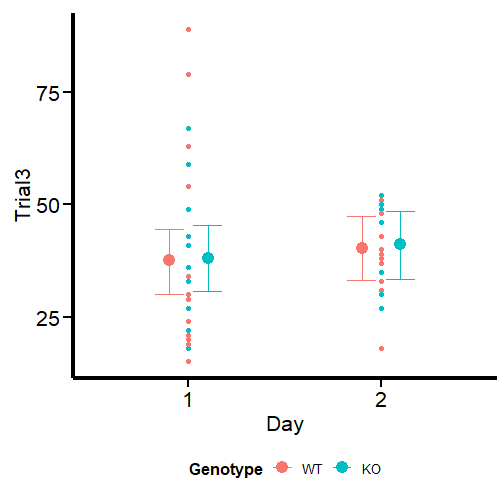
So, let’s skip data simulations and get serious. We’ll work with real data I have acquired from mice performing the rotarod test.
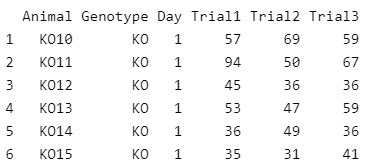
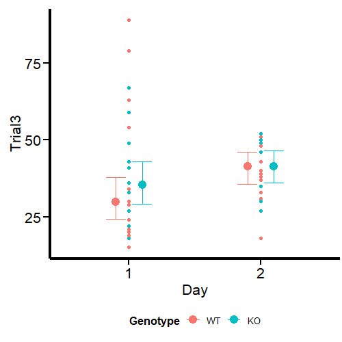
First, we load the dataset into our environment and set the corresponding factor levels. The dataset contains IDs for the animals, a groping variable (Genotype), an indicator for two different days on which the test was performed (day), and different trials for the same day. For this article, we model only one of the trials (Trial3). We will save the other trials for a future article on modeling variation.
As the data handling implies, our modeling strategy will be based on Genotype and Day as categorical predictors of the distribution of Trial3.
In biomedical science, categorical predictors, or grouping factors, are more common than continuous predictors. Scientists in this field like to divide their samples into groups or conditions and apply different treatments.
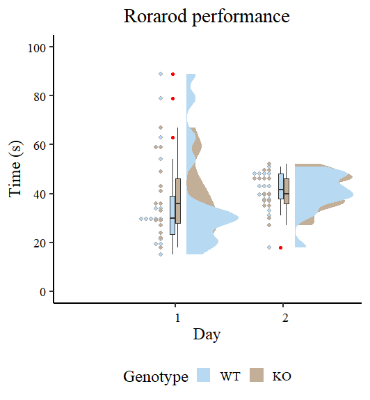
Figure 2 looks different from the original by Guilherme A. Franchi, PhD because we are plotting two factors instead of one. However, the nature of the plot is the same. Pay attention to the red dots, these are the ones that can be considered extreme observations that tilt the measures of central tendency (especially the mean) toward one direction. We also observe that the variances are different, so modeling also sigma can give better estimates. Our task now is to model the output using the brms package.
Fitting statistical models with brms
Here we fit our model with Day and Genotype as interacting categorical predictors for the distribution of Trial 3. Let’s first fit a typical Gaussian model, which is analogous to an ordinary least squares (OLS) model from the frequentist framework, since we are using the default flat brms priors. Priors are beyond the scope of this article, but I promise we’ll cover them in a future blog.
Once we have results from the Gaussian model, we can compare them to the large results from the Student’s t model. We then addsigma to the equation to account for the difference in the variance of the data.
Fitting a “typical” (frequentists) model in Gaussian land
Our Gaussian model is built under the typical (and often incorrect) assumption of homoscedasticity (3). In other words, we assume that all groups have the same (or very similar) variance. I do not recall seeing this as a researcher.
Gaussian_Fit1 <- brm(Trial3 ~ Day * Genotype,
           data = data,
           family = gaussian(),
           # seed for reproducibility purposes
           seed = 8807,
           control = list(adapt_delta = 0.99),
           # this is to save the model in my laptop
           file    = "Models/20240222_OutliersStudent-t/Gaussian_Fit1.rds",
           file_refit = "never")

# Add loo for model comparison
Gaussian_Fit1 <-
  add_criterion(Gaussian_Fit1, c("loo", "waic", "bayes_R2"))
Model diagnostics
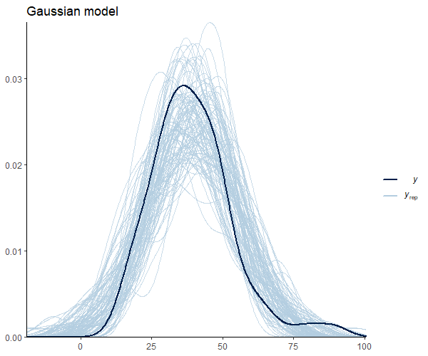
Before proceeding, it’s a good idea to do some simple model diagnostics to compare the actual observations with the predictions made by our model. We can do this in several ways, but the most common is to plot full densities. We can achieve this using the pp_check function from brms.
Figure 3 suggests that our observations (dark blue) are not meaningfully different from the model predictions. Below, I leave you with additional code to check other pp_check alternatives with their respective graphs.
set.seed(88071)

pp_check(Gaussian_Fit1, group = "Genotype", type = "dens_overlay_grouped", ndraws = 100) +
  labs(title = "Density by Genotype") +
    theme_classic()

pp_check(Gaussian_Fit1, type = "stat_grouped", group = "Genotype", stat = "var", binwidth = 3) +
  coord_cartesian(xlim = c(0, 300)) +
  ggtitle("Grouped variance") +
  theme_classic()

pp_check(Gaussian_Fit1, type = "stat", stat = "var", binwidth = 3) +
  coord_cartesian(xlim = c(0, 600)) +
  ggtitle("How well we captured the variace") +
  theme_classic()

pp_check(Gaussian_Fit1, type = "stat", stat = "mean", binwidth = 2) +
  coord_cartesian(xlim = c(0, 50)) +
  ggtitle("How well we captured the mean") +
  theme_classic()
Checking the results for the Gaussian distribution
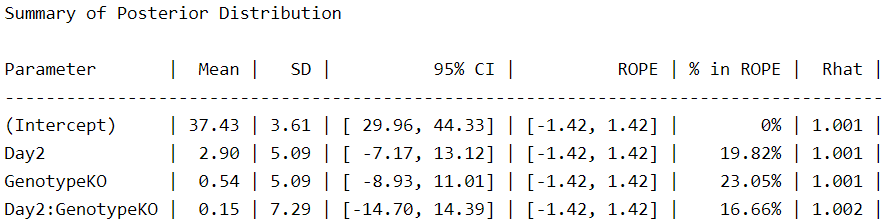
Now, we use the describe_posterior function from the bayestestR package (4) to see the results:
Let’s focus here on the ‘intercept’, which is the value for WT at 1 DPI, and ‘GenotypeKO’, the estimated difference for KO animals at the same time point. We see that WT animals spend about 37 seconds in the rotarod, while their KO counterparts spend less than a second (0.54) more. As a researcher in this field, I can say that this difference is meaningless and that genotype has no effect on rotarod performance. Even the effect of day, which is 2.9, seems meaningless to me under this model. We can easily visualize these estimates using the wonderful conditional_effects function from brms.
# We create the graph for convex hull Gaussian_CondEffects <- conditional_effects(Gaussian_Fit1)
Figure 8: Conditional effects for the Gaussian model
In Figure 8 we can see the estimates and uncertainty for the interaction terms. I have customized the plot with a number of ggplot elements, which you can check in the original Quarto Notebook. Note the similar uncertainty for both time points, even though the dispersion is larger on day 1 than on day 2. We will address this point in a small snippet at the end of this article.
Now let’s see how much our understanding changes when we model the same data using a student-t distribution.
Fitting our guest: a model with a student-t distribution
It’s time to use the student-t distribution in our `brms` model.
Student_Fit <- brm(Trial3 ~ Day * Genotype,
           data = data,
           family = student,
           # seed for reproducibility purposes
           seed = 8807,
           control = list(adapt_delta = 0.99),
           # this is to save the model in my laptop
           file    = "Models/20240222_OutliersStudent-t/Student_Fit.rds",
           file_refit = "never")

# Add loo for model comparison
Student_Fit <-
  add_criterion(Student_Fit, c("loo", "waic", "bayes_R2"))
Model diagnostics
We plot the model diagnostics as done before:
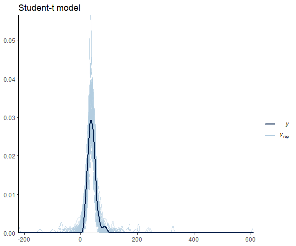
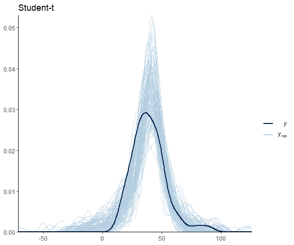
Figure 9: Model diagnostics for student-t distribution
Figure 9 shows that the mean shape and the peak of the observations and the predictions match. It’s important to note that our model seems to predict values below 0. This is an important research issue that we will skip for now. However, it does imply the use of informative priors or distribution families that set a lower bound at 0, such as the log_normal’,hurdle_lognormal’, or `zero_inflated_poisson’, depending on the case. Andrew Heiss (5) offers a great example in this regard.
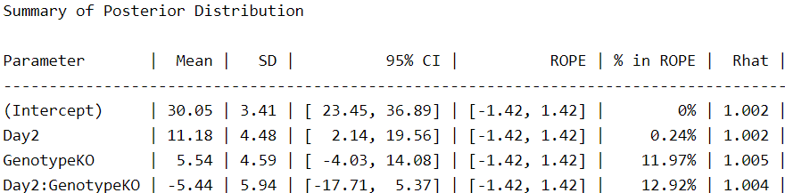
Checking the results for the student-t distribution
Under this model, we can see that our estimates have changed moderately, I would say. Our estimate for the intercept (WT at 1 day) is reduced by 7 seconds. And why is that? Because the extreme values we discovered at the beginning have less influence on the measures of central tendency of the data. Thus, this is a more accurate measure of the “typical” WT animal on day 1. We also observe a substantial increase in the effect of day, with almost 10 seconds more than our initial Gaussian estimates. Importantly, the effect of our KO genotype appears to be more notorious, increasing about 10 times from 0.52 in our Gaussian model to 5.5 in our student-t model. From my perspective, given the context of these data, the contrasts between the two models are notorious.
Let’s see it in graphical terms using conditional_effects:
Figure 10: Conditional effects for the Student-t model
Can we get better estimates? For this particular example, I think we can. From the start, it was easy to notice the difference in the variance of the data, especially when we compare the first and second-day visuals. We improved our estimates using the student-t distribution, and we can improve them further by developing a model for heteroscedasticity that predicts sigma (the residual variance).
In this way, the model does not assume that your residual variance is equal across your grouping variables, but it becomes a response that can be modeled by predictors.
This is the little point we left for the end.
Predicting sigma using a student-t distribution
We include sigma as a response variable using thebf function from brms. In this case, we are going to model this parameter using the same predictors Day and Genotype.
Student_Mdl2 <- bf (Trial3 ~ Day * Genotype,
                     sigma ~ Day * Genotype)

Student_Fit2 <- brm(
           formula = Student_Mdl2,
           data = data,
           family = student,
           # seed for reproducibility purposes
           seed = 8807,
           control = list(adapt_delta = 0.99),
           # this is to save the model in my laptop
           file    = "Models/20240222_OutliersStudent-t/Student_Fit2.rds",
           file_refit = "never")

# Add loo for model comparison
Student_Fit2 <-
  add_criterion(Student_Fit2, c("loo", "waic", "bayes_R2"))
Model diagnostics
Figure 11: Model diagnostics for student-t distribution with sigma
Figure 11 looks good, except for the uncomfortable predictions below 0. For this case, I judge that this does not strongly bias the estimates and their uncertainty. However, this is an aspect I will take into account when doing actual research.
Checking the results for the student-t distribution with predicted sigma
Now, let’s take a look at the posterior distribution.
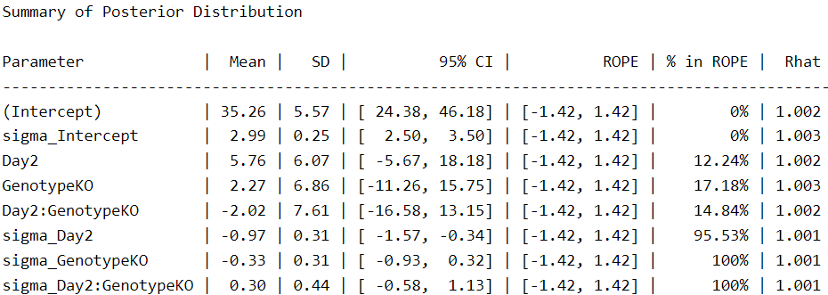
We see more parameters compared to the other two fitted models because the response for sigma is now included as a main effect in the model. Under this scheme, we see that the intercepts are closer to those of the Gaussian model and the effect of genotype (GenotypeKO) is reduced by half.
There is one aspect to note, however. In our first Student-t model, the uncertainty for the intercept was 24.1–37.4. On the other hand, in the last model, the uncertainty increases to 24.3–46.1. This means that when we consider the different variances, we are less certain of this (and other) parameters. The same is true for day, for example, which changes from 1.2–18.9 to -5.6–18.1. In this case, we are now less certain that the second day is associated with an increase in time spent on the rotarod.
Don’t worry, the purpose of statistical modeling is to provide the best possible quantification of the uncertainty in a measurement, and that’s what we’re doing right now. Of course, our uncertainty increases when we have extreme values that are part of our sample and therefore part of our population.
In this example, we see that accounting for the different variances in our data gives us a very different idea of our results.
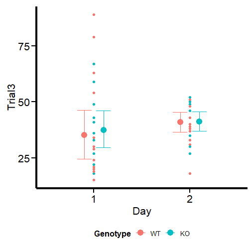
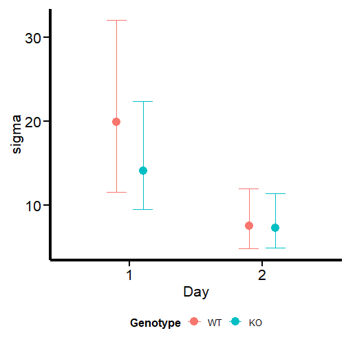
Finally, we can see that sigma, plotted on the log scale, varies meaningfully with day and genotype:
Figure 12: Conditional effects for the Student-t model with sigmaFigure 13: Conditional effects for sigma
What we see in the second graph is sigma, which effectively accounts for the variance in this parameter between days and genotypes. We see a much higher uncertainty at day 1, especially for WT mice, while the parameter is analogous at day 2.
We can conclude this article by comparing the three models for out-of-sample predictions.
Model comparison
We perform model comparisons using the WAIC criteria (6)for estimating the out-of-sample prediction error. By considering both the log-likelihood of the observed data and the effective number of parameters, it provides a balance between model fit and complexity. Unlike some other criteria, WAIC inherently accounts for the posterior distribution of the parameters rather than relying on point estimates, making it particularly suited to Bayesian analyses.
Given a data set and a Bayesian model, the WAIC is calculated as:
WAIC=−2×(LLPD−pWAIC)
Where: LLPD is the log pointwise predictive density, calculated as the average log-likelihood for each observed data point across the posterior samples. WAIC is the effective number of parameters, computed as the difference between the average of the log-likelihoods and the log-likelihood of the averages across posterior samples.
We use the compare_performance function from the performance package, part of the easystats environment (4, 7, 8).
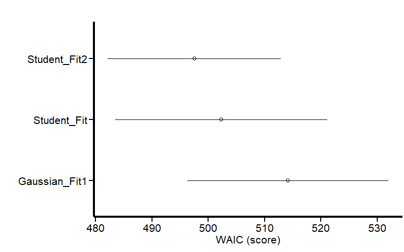
The output shows that our Student-t model predicting sigma is the least penalized (WAIC = 497) for out-of-sample prediction. Note that there is no estimate for sigma in this model because it was included as a response variable. This table also shows that the student-t model has less residual variance (sigma) than the Gaussian model, which means that the variance is better explained by the predictors. We can visualize the same results as a graph:
) + coord_flip() + labs(x = "", y = "WAIC (score)", title = "") + Plot_theme
Fit_Comp_WAIC
Figure 14: Model comparison by WAIC
Figure 14 shows that our last model is less penalized for out-of-sample prediction.
You can find an updated version of this post on my GitHub site. Let me know if this journey was useful to you, and if you have any constructive comments to add to this exercise.
*Unless otherwise noted, all images are generated by the author using R code.
References
1.M. Ahsanullah, B. M. G. Kibria, M. Shakil, Normal and student´s t distributions and their applications (Atlantis Press, 2014; http://dx.doi.org/10.2991/978-94-6239-061-4).
2. P.-C. Bürkner, Brms: An r package for bayesian multilevel models using stan. 80 (2017), doi:10.18637/jss.v080.i01.
5. A. Heiss, A guide to modeling proportions with bayesian beta and zero-inflated beta regression models (2021), (available at http://dx.doi.org/10.59350/7p1a4-0tw75).
Let me introduce you to Sarah, a talented and passionate data scientist, who just landed her dream job at GreenEnv, a large company that makes eco-friendly cleaning products. GreenEnv has tons of data on customers, products, and other areas of the business. They hired Sarah to unlock the hidden potential within this data, uncovering market trends, competitive advantages, and more.
Her first task: analyze customer demographics and buying habits to create targeted marketing campaigns. Confident in her abilities and excited to apply data science methods, Sarah dived into the customer database. But her initial excitement quickly faded. The data was a mess — inconsistent formatting, misspelled names, and duplicate entries everywhere. Data quality was terrible. There were variations of names like “Jhon Smith” and “Micheal Brown” alongside entries like “Jhonn Smtih” and “Michealw Brown.” Emails had extra spaces and even typos like “gnail.com” instead of “gmail.com.” along with many other inaccuracies. Sarah realized the hard job ahead of her — data cleaning.
Inconsistent formatting, missing values, and duplicates would lead to skewed results, giving an inaccurate picture of GreenEnv’s customer base. Days turned into weeks as Sarah tirelessly cleaned the data, fixing inconsistencies, filling in gaps, and eliminating duplicates. It was a tedious process, but essential to ensure her analysis was built on a solid foundation.
Who cares about data quality?
Every year, poor data quality costs organizations an average of $12.9 million. [1]
Thankfully, after weeks of cleaning and organizing this messy data, Sarah was able to get the job done…or at least for this part..
Her next challenge came when she ventured into product data, aiming to identify top-selling items and recommend future opportunities. However, she encountered a different problem — a complete lack of metadata. Product descriptions were absent, and categories were ambiguous. Basically, there wasn’t enough data to help Sarah to understand the product’s data. Sarah realized the importance of metadata management — structured information about the data itself. Without it, understanding and analyzing the data was almost impossible.
Research Shows Most Data Has Inaccuracies
Research by Experian reveals that businesses believe around 29% of their data is inaccurate in some way. [2]
Frustrated but determined, Sarah reached out to different departments to piece together information about the products. She discovered that each department used its own internal jargon and classification systems. Marketing and sales refer to the same cleaning product with different names.
As Sarah delved deeper, she found that datasets were kept in separate applications by different departments, outdated storage systems struggling to handle the growing volume of data, and Sarah had to wait for a long time for her queries to be executed. Sarah noticed also there are no clear rules on who can access what data and under what terms, without centralized control and proper access controls, the risk of unauthorized access to sensitive information increases, potentially leading to data breaches and compliance violations. The lack of data governance, a set of rules and procedures for managing data, was evident.
Data Breaches Can Be Costly
According to the Ponemon Institute, the average cost of a data breach in 2023 is $4.45 million globally, an all-time high record, with costs varying by industry and location. [3]
Each of the above issues and hurdles in Sarah’s story highlighted the interconnectedness of many pillars — data quality, metadata management, and data governance all played a crucial role in accessing and utilizing valuable insights at GreenEnv.
Sarah’s journey is a common one for data scientists and analysts. Many organizations have massive amounts of data, and everyone knows the saying: “Data is the new electricity.” Every organization wants to make the most of their data, as it’s a very valuable asset. But most people mistakenly (and practically) believe that simply hiring a data analyst or data scientist is enough to unlock this value. There are many pillars to getting the most value from data, and organizations need to account for and pay attention to these. The keyword here is data management.
Did you know..
86% of organizations say they believe investing in data management directly impacts their business growth[4]
What Exactly is Data Management?
Generally speaking, data management is the overall practice of handling the organization’s data. from acquiring and storing the data to processing, securing, and analyzing it. The goal is to ensure the data is accessible, usable, accurate, reliable, and of high quality to achieve the state of data-informed organization and ultimately achieve our organizational objectives.
The Pillars of Data Management
There are several key dimensions that work together to achieve successful data utilization, and while these pillars might be slightly different from one framework to another, the underlying concepts are the same.
In addition to data security and data integration as pillars we also have:
Data Quality: This ensures the data is accurate, consistent, complete, and timely. It involves identifying and fixing errors, managing missing values, and establishing data cleaning and validation processes.
Metadata Management: This focuses on organizing and cataloging information about the data itself.
Data Governance: This establishes the framework and rules for managing data assets throughout their lifecycle. It involves setting policies, and processes, and assigning roles to ensure data accuracy, security, and compliance with regulations.
Data Architecture: This defines the structure and organization of data assets. It includes defining data models, storage solutions, and data flows, ensuring efficient data storage, retrieval, and utilization.
Data Lifecycle Management: This focuses on managing data throughout its entire lifespan, from creation to archiving or deletion. It involves implementing processes for data capture, storage, transformation, use, and disposal.
You can notice that these dimensions are interconnected and also closely related. Addressing weaknesses in one area can often impact others. Some frameworks have been developed to address the relationship between the different dimensions of data management and how they interact and affect each other.
Data Management Frameworks: The Aiken’s Pyramid
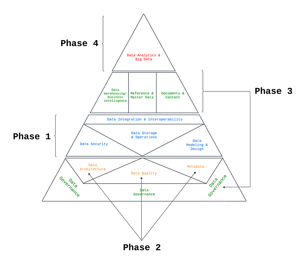
Aiken’s Pyramid: Image by Author
Many established frameworks like DAMA-DMBOK2, IGF, and EDM offer structured guidance, standardized terminology, and maturity assessments for data management
One conceptual framework worth mentioning here, and the one I like the most, is Aiken’s pyramid of Data Management. It outlines the different stages of data management processes. Developed by Robert Aiken, a data management pioneer, this framework describes the situation in which many organizations find themselves. In trying to leverage the full potential of their data, many organizations go through a similar progression of steps:
Phase 1: This focuses on establishing the basic building blocks, like data modeling, storage solutions, and security measures.
Phase 2: As data usage increases, this level addresses challenges arising from poor data quality and activities like metadata management and data architecture.
Phase 3: The previous activities from Phase 2 require data governance. data governance also enables activities like document and content management, reference and master data management, data warehousing, and business intelligence, all in turn allowing for advanced analytics in Phase 4.
Phase 4: This is the stage where the organization truly unlock the full potential of their data. Here, organizations leverage high-quality data for advanced analytics and data science and extract valuable insights to inform decision-making.
The Aiken Pyramid helps organizations understand how data management activities interconnect, how each one builds on the others, and how to prioritize their efforts for effective data utilization.
My Reflections and Takeaways on Data Management Best Practices
Reflecting on learning and experience with data management(although I’m not a data management expert XD), I’ve come to appreciate and favor the following points regarding data management and its best practices, especially if we are focusing on data quality.
There’s no one-size-fits-all solution to data management. While frameworks exist to guide organizations towards data management maturity, the full process remains unique for each entity. Each organization prioritizes different aspects of data management and faces distinct challenges.
My approach would be to start simple. Apply data management best practices or enhancements to a targeted portion of the organization’s data, focusing on what matters most. This allows for gradual growth in maturity, eventually encompassing all data. This phased approach can be very beneficial for dimensions like data quality and metadata management.
If a process consistently generates bad data, even the best efforts in other areas of data management won’t prevent it. These processes can be technical or non-technical. A proactive approach is crucial here.
– For example, a non-technical process that generates bad data might involve database creation by developers who solely focus on the technical aspects. There might be a lack of documentation or column descriptions for instance. A good practice in my opinion would be to engage data analysts and other relevant stakeholders in the design process to ensure adherence to data management best practices. The data management team can decide if we would go forward with a certain application design or not.
– An application’s design can also be a technical process for bad data generation. A well-designed application should enforce data quality proactively during data entry. For instance, instead of a text box for entering gender, a dropdown menu could be used. Another example might be predefining email types, where the user only needs to add their username before automatically receiving “@gmail.com” or another domain extension.
Standardization is key: Inconsistency in data can be a nightmare. Imagine customer names stored differently across departments, dates in conflicting formats, or teams using their own abbreviations. but more than that within a single organization or a company there might be different processes that generate the same type of data, and different data collection tools. Standardization combats this chaos by establishing common formats, definitions, and processes for data handling. This ensures data quality, simplifies integration across applications, fosters collaboration through a shared data language, and boosts efficiency by streamlining data workflows. This process is also iterative and agile, the organization can gradually achieve more levels of maturity in it. This one can also be part of the previous data management process of validation of applications that generate data: adherence to standards. i.e. any application to be approved should comply to the standards first.
Finally, data management is a comprehensive process that requires collaboration across different teams within the organization, with the need to define the data management strategy and align it with the business or institute’s objectives and strategies. This would typically start with assessing the current and desired data management maturity levels, analyzing the gap, prioritizing data management tasks, and remaining agile. The process is iterative, and clear solutions rarely exist in advance.
Data Management Professional Career
There are many data management certifications out there you might consider. The best choice depends on your specific goals and experience but here are a few ones I came across:
Certified Data Management Professional (CDMP): Offered by the Data Management Association (DAMA) International, this covers a wide range of topics, from data governance and quality to modeling.
Certified Information Management Professional (CIMP): This program, offered by the Institute for Information Management (IIM), focuses on information management disciplines like governance, quality, security, and more.
Data Governance and Stewardship Professional (DGSP): This certification, from the Data Governance Institute, focuses on the skills needed to develop and implement a data governance program, along with ensuring data quality, compliance with regulations, and so on.
Certified Clinical Data Manager (CCDM): This one, offered by the Society for Clinical Data Management (SCDM), is for professionals in clinical research who manage data collected during trials.
Ultimately the choice of which one is worth the time and effort requires a more in-depth analysis of the credibility, content, and purpose of each certification.
Looking Ahead: Data Management Tools
Image by author
As you would guess, there is an endless number of tools available to address different aspects of data management, and it would be impractical to talk about all these tools, each tool would have pros and cons, and situations where it might be effective, or specific data management dimensions where it would be helpful.
In my next article, I will delve deeper into two open-source tools for data management, DataHub and Great Expectations(GX), and provide a step-by-step guide on how to integrate them to create a robust, cost-effective, scalable, and unified environment for data discovery, metadata management, data quality, data governance, data lineage, and impact analysis.
Conclusion
Data is arguably an organization’s most valuable asset these days. However, many still lack proper data management, limiting their ability to leverage its true potential. Issues like data quality, governance, security, and metadata management are all central pillars to get the most value out of your organization’s data.
Remember Sarah’s story at the beginning? Hiring a data scientist isn’t enough. They often spend a significant amount of time cleaning and organizing messy data before they can even begin analysis. Thankfully, frameworks like the Aiken Pyramid can guide organizations on their data management journey, and help in communicating data management initiatives across the different teams and different stakeholders easily and regardless of their technical level.
Thanks for reading all the way here! I hope you found this informative and enjoyable. Please feel free to point out any mistakes or share your thoughts — your feedback is always appreciated.
References
Gartner. (2021). “How to Improve Your Data Quality.” Smarter With Gartner, Gartner”
Experian. (2019). “Global Data Management Research Report.”
Ponemon Institute. (2023). “Cost of a Data Breach Report.”
Experian. (2021), “Data experience The data-driven strategy behind business growth report”
Further Readings
Books
Data Management Body of Knowledge (DAMA-DMBOK): The DAMA-DMBOK 2nd edition, this one serves as a comprehensive guide to data management practices and principles. It provides a detailed overview of various aspects of data management. [my favorite reference for data management!]
“Data Governance: How to Design, Deploy and Sustain an Effective Data Governance Program” by John Ladley.
“The Case for the Chief Data Officer: Recasting the C-Suite to Leverage Your Most Valuable Asset”, by Peter Aiken, Michael M. Gorman
“Data Management for Researchers: Organize, Maintain and Share Your Data for Research Success” by Kristin Briney.
Online Resources:
Data Management Association (DAMA) International: DAMA International offers a wealth of resources on data management, including articles, webinars, and whitepapers. Their website is a valuable resource for both beginners and experienced professionals.
CDMP Study Group on Facebook: Here you can find many data practitioners and others who are interested in the CDMP exam, you can ask questions, seek a study partner, or join them in their regular webinars and discussions about data management based on the CDMP topics. personally, this one is one of my favorites, thanks to Nicole Janeway Bills for her efforts in this group.
We use cookies on our website to give you the most relevant experience by remembering your preferences and repeat visits. By clicking “Accept”, you consent to the use of ALL the cookies.
This website uses cookies to improve your experience while you navigate through the website. Out of these, the cookies that are categorized as necessary are stored on your browser as they are essential for the working of basic functionalities of the website. We also use third-party cookies that help us analyze and understand how you use this website. These cookies will be stored in your browser only with your consent. You also have the option to opt-out of these cookies. But opting out of some of these cookies may affect your browsing experience.
Necessary cookies are absolutely essential for the website to function properly. These cookies ensure basic functionalities and security features of the website, anonymously.
Cookie
Duration
Description
cookielawinfo-checkbox-analytics
11 months
This cookie is set by GDPR Cookie Consent plugin. The cookie is used to store the user consent for the cookies in the category "Analytics".
cookielawinfo-checkbox-functional
11 months
The cookie is set by GDPR cookie consent to record the user consent for the cookies in the category "Functional".
cookielawinfo-checkbox-necessary
11 months
This cookie is set by GDPR Cookie Consent plugin. The cookies is used to store the user consent for the cookies in the category "Necessary".
cookielawinfo-checkbox-others
11 months
This cookie is set by GDPR Cookie Consent plugin. The cookie is used to store the user consent for the cookies in the category "Other.
cookielawinfo-checkbox-performance
11 months
This cookie is set by GDPR Cookie Consent plugin. The cookie is used to store the user consent for the cookies in the category "Performance".
viewed_cookie_policy
11 months
The cookie is set by the GDPR Cookie Consent plugin and is used to store whether or not user has consented to the use of cookies. It does not store any personal data.
Functional cookies help to perform certain functionalities like sharing the content of the website on social media platforms, collect feedbacks, and other third-party features.
Performance cookies are used to understand and analyze the key performance indexes of the website which helps in delivering a better user experience for the visitors.
Analytical cookies are used to understand how visitors interact with the website. These cookies help provide information on metrics the number of visitors, bounce rate, traffic source, etc.
Advertisement cookies are used to provide visitors with relevant ads and marketing campaigns. These cookies track visitors across websites and collect information to provide customized ads.