TLDR: I have created an experiment — iterating through various shoe types to achieve Eliud Kipchoge Running Efficiency. By surprise — it…
Originally appeared here:
Running Efficiency with Computer Vision: A Comparative Analysis with Eliud Kipchoge

TLDR: I have created an experiment — iterating through various shoe types to achieve Eliud Kipchoge Running Efficiency. By surprise — it…
Originally appeared here:
Running Efficiency with Computer Vision: A Comparative Analysis with Eliud Kipchoge
Looking to speed up your data processing pipelines up to 10 times? Maybe it’s time to say goodbye to Pandas.
Originally appeared here:
Pandas vs. Polars — Time to Switch?
Go Here to Read this Fast! Pandas vs. Polars — Time to Switch?

In neuroscience and other biomedical sciences, it is common to use behavioral tests to assess responses to experimental conditions or treatments. We can assess many aspects, from basic motor and exploratory behaviors to memory and learning. Many of these variables are continuous (numerical) responses, i.e. they can take (finite or infinite) values in a given range. Time in the open field, animal weight, or the number of cells in a brain region are some examples.
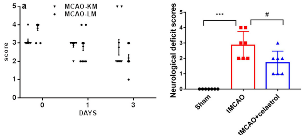
However, there are other types of variables that we record in our experiments. A very common one is ordered categorical variables, also called ordinal variables. These are categorical variables that have a natural order, analogous to the well-known surveys in which we answer whether we agree or disagree with a statement, with 0 being strongly disagree and 5 being strongly agree. To facilitate the recording of these variables in printed or digital datasheets, we codify them (by convention) as numbers. This is the case of the 5-point Bederson score used in the context of cerebral ischemia research in rodent models (1), which is coded as follows:
– 0 = no observable deficit
– 1 = forelimb flexion
– 2 = forelimb flexion and decreased resistance to lateral push
– 3 = circling
– 4 = circling and spinning around the cranial-caudal axis
– 5 = no spontaneous movement.
Note that the numbers are just simple conventions. We could also use a,b,c,d,e; excellent, good, not so good, bad, very bad, almost dead; etc. I do not think it is presumptuous to stress the self-evident nature of the matter.
Surprisingly, however, Figure 1 represents a particular and widespread malpractice that scientists in this field have been practicing for years: They use t-tests and ANOVAS to analyze such ordered categorical variables.
I still cannot find a logical explanation for why dozens of authors, reviewers, and editors feel comfortable with this scenario. Not only is it not logical, but more importantly, it leads to biased effect sizes, low detection rates, and type I error rates, among other things (2).
When I have played the role of reviewer 2 and emphasized this point to authors, asking them why they evaluate a categorical response with a statistical test designed to deal with continuous numerical variables, what I get is a long list of published articles that follow this irrational practice. So I finally found an answer to why they do it:
what Gerd Gigerenzer (2004) calls “the ritual of mindless statistics” (3).
In fact, most of us scientists have little idea what we are doing with our data, and are simply repeating common malpractices passed down from generation to generation in labs around the world.
In this article, we’ll then look at a more viable alternative for analyzing ordered categorical variables using R, brms (4) and elements from the tidyverse (5).
To avoid the ritual of mindless statistics, we’ll recreate the data set from Liu et. al (2022) in Figure 1 by eyeballing the data points and organizing them in a table:
# We Define the observations
observations <- list(
  Sham = c(rep(0, 7)),
  tMCAO = c(rep(2, 3), rep(3, 2), rep(4, 2)),
  tMCAO_C = c(rep(1, 3), rep(2, 3), rep(3, 1))
)

# We create an empty data frame to populate
df <- data.frame(Group = character(), Response = integer())

# We populate the data frame
for (group in names(observations)) {
  for (response in unique(observations[[group]])) {
    df <- rbind(df, data.frame(Group = rep(group, sum(observations[[group]] == response)),
                               Response = rep(response, sum(observations[[group]] == response))))
  }
}

head(df)
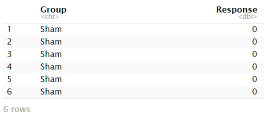
If you look at the R code (in R-studio) at this point, you will notice that the variable `Response’ is identified as a number ranging from 0 to 4. Of course, we are fully aware that this response is not numeric, but an ordered (ordinal) categorical variable. So we do the conversion explicitly:
df$Response <- factor(df$Response, levels = c("0", "1", "2", "3", "4"), ordered = TRUE)

str(df)

Now we can verify that it is recognized as an ordered categorical variable. With this in hand, we can easily move on to visualization and modeling.
First, let’s load the necessary libraries and create a visual theme for our plots.
library(ggplot2)
library(brms)
library(ggdist)
library(easystats)
library(dplyr)
library(tibble)

Plot_theme <- theme_classic() +
  theme(
      plot.title = element_text(size=18, hjust = 0.5, face="bold"),
      plot.subtitle = element_text(size = 10, color = "black"),
      plot.caption = element_text(size = 12, color = "black"),
      axis.line = element_line(colour = "black", size = 1.5, linetype = "solid"),
      axis.ticks.length=unit(7,"pt"),

      axis.title.x = element_text(colour = "black", size = 16),
      axis.text.x = element_text(colour = "black", size = 16, angle = 0, hjust = 0.5),
      axis.ticks.x = element_line(colour = "black", size = 1),

      axis.title.y = element_text(colour = "black", size = 16),
      axis.text.y = element_text(colour = "black", size = 16),
      axis.ticks.y = element_line(colour = "black", size = 1),

      legend.position="right",
      legend.direction="vertical",
      legend.title = element_text(colour="black", face="bold", size=12),
      legend.text = element_text(colour="black", size=10),

      plot.margin = margin(t = 10,  # Top margin
                             r = 2,  # Right margin
                             b = 10,  # Bottom margin
                             l = 10) # Left margin
      )
A simple way to visualize categorical data is with a bar graph.
ggplot(df, aes(x = factor(Response), fill = Group)) +
  geom_bar(position = "dodge") +
  labs(x = "Response", y = "Count", title = "Response by Group") +
  theme_minimal() +
  scale_fill_brewer(palette = "Set1") +
  Plot_theme +
theme(legend.position = "top", legend.direction = "horizontal")
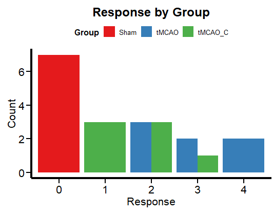
Figure 2 shows the frequency per group. This is more in line with the logic of a categorical variable than box plots, which are more relevant for continuous numerical variables. Now let’s run a regression to unravel the mysteries (if any) of this data set.
We’ll use brms to fit a cumulative model. This model assumes that the neurological score Y is derived from the categorization of a (presumably) latent (but not observable or measured) continuous variable Y˜ (2). As usual in most brms tutorials, I must apologize for skipping the “priors” issue. Let’s assume an “I have no idea” mentality and let the default (flat) brms priors do the dirty work.
We fit the cumulative model by following the usual formula syntax and adding cumulative(“probit”) as a family (assuming the latent variable and the corresponding error term are normally distributed). We have only one predictor variable, the experimental group to which each animal belongs.
Ordinal_Fit <- brm(Response ~ Group,
           data = df,
           family = cumulative("probit"),
           # seed for reproducibility purposes
           seed = 8807,
           control = list(adapt_delta = 0.99),
           # this is to save the model in my laptop
           file    = "Models/2024-04-03_UseAndAbuseANOVA/Ordinal_Fit.rds",
           file_refit = "never")

# Add loo for model comparison
Ordinal_Fit <-
  add_criterion(Ordinal_Fit, c("loo", "waic", "bayes_R2"))
Before we look at the results, let’s do some model diagnostics to compare the observations and the model predictions.
pp_check(Ordinal_Fit, ndraws = 100) +
  labs(title = "Ordinal regression") +
  theme_classic()
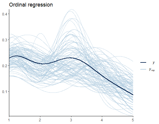
From Figure 3, I speculate that such deviations are the results of the uneven distribution (variance) of scores across groups. Later, we’ll see if predicting the variance yields better estimates. For now, we are good to go.
Let’s take a look at the posterior distribution using the describe_posterior function from the bayestestR package (6), as an alternative to the typical summary function.
describe_posterior(Ordinal_Fit,
                   centrality = "mean",
                   dispersion = TRUE,
                   ci_method = "HDI",
                   test = "rope",
                   )
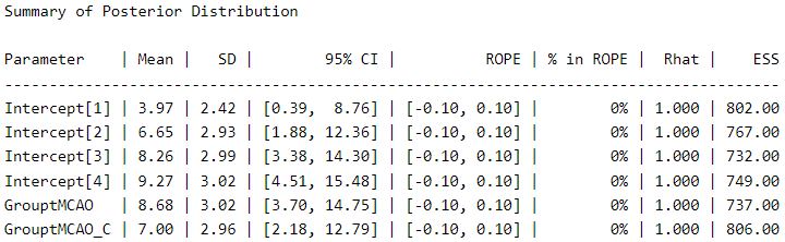
The thresholds (score thresholds) are labeled as “Intercepts” in this model, which apply to our baseline “sham” condition. The coefficients for “GrouptMCAO” and “GrouptMCAO_C” indicate the difference from sham animals on the latent Y˜ scale. Thus, we see that “GrouptMCAO” has 8.6 standard deviations higher scores on the latent Y˜ scale.
I want to point out a crucial (and not trivial) aspect here as a reminder for a future post (stay tuned). In my opinion, it is irrelevant to make comparisons between a group that does not have a distribution (which is 0 in all cases), such as the sham group, and a group that does have a distribution (the experimental groups). If you think about it carefully, the purpose of this procedure is null. But let us follow the thread of modern scientific culture and not think too much about it.
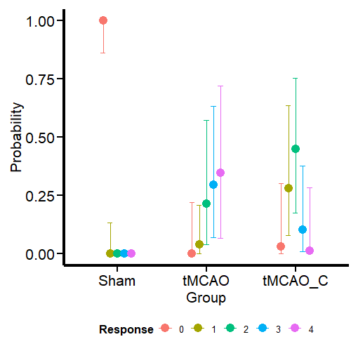
Of course, appreciating the difference between the groups becomes more feasible if we look at it visually with the conditional effects’ function ofbrms’.
Ordinal_CondEffects <-
  conditional_effects(Ordinal_Fit, "Group", categorical = TRUE)

Ordinal_CondEffects <- plot(Ordinal_CondEffects,
       plot = FALSE)[[1]]

Ordinal_CondEffects +
  Plot_theme +
  theme(legend.position = "bottom", legend.direction = "horizontal")
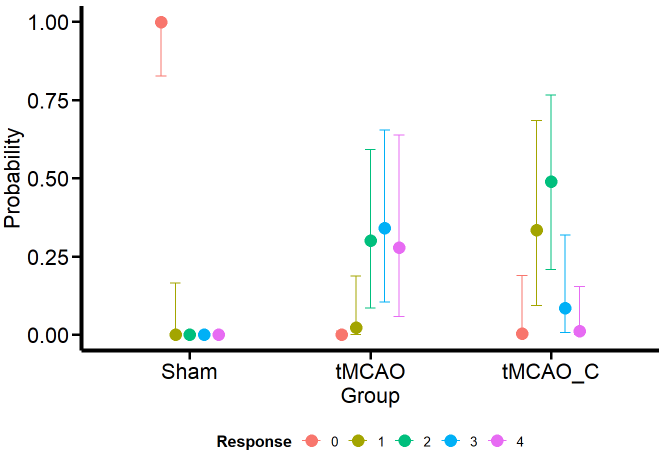
Curiously (or perhaps not so much from the MCMC simulation framework), the model estimates that the dummy group can have values of 1, although we have not seen this in the data. One possible reason is that the model estimates a common variance for all groups. We’ll see if this aspect changes when we model the variance as a response.
Otherwise, the estimates obtained for the tMCAO and tMCO_C groups are much closer to the data. This allows us to make more precise statements instead of running an ANOVA (incorrectly for ordinal variables) and saying that there is “a significant difference” between one group and the other, which is a meaningless statement. For example, the model tells us that scores of 2–4 for the tMCAO group have a similar probability (about 25%). The case is different for the tMCAO_C group, where the probability of 2 in the neurological score is higher (with considerable uncertainty) than for the other scores. If I were confronted with this data set and this model, I would claim that the probability that the tMCAO_C group reflects less neurological damage (based on scores 1 and 2) is higher than for the tMCAO group.
Can we get precise numbers that quantify the differences between the scores of the different groups and their uncertainty? Of course, we can! using the emmeans package (7). But that will be the subject of another post (stay tuned).
For this type of cumulative model, there is no sigma parameter. Instead, to account for unequal variances, we need to use a parameter called disc. For more on this aspect, see the Ordinal Regression tutorial by Paul-Christian Bürkner, the creator of brms (2).
Ordinal_Mdl2 <- bf (Response ~ Group) +
                     lf(disc ~  0 + Group, cmc = FALSE)

Ordinal_Fit2 <- brm(
           formula = Ordinal_Mdl2,
           data = df,
           family = cumulative("probit"),
           # seed for reproducibility purposes
           seed = 8807,
           control = list(adapt_delta = 0.99),
           # this is to save the model in my laptop
           file    = "Models/2024-04-03_UseAndAbuseANOVA/Ordinal_Fit2.rds",
           file_refit = "never")

# Add loo for model comparison
Ordinal_Fit2 <-
  add_criterion(Ordinal_Fit2, c("loo", "waic", "bayes_R2"))
We perform the model diagnostics as done previously:
pp_check(Ordinal_Fit2, ndraws = 100) +
  labs(title = "Student-t") +
  theme_classic()
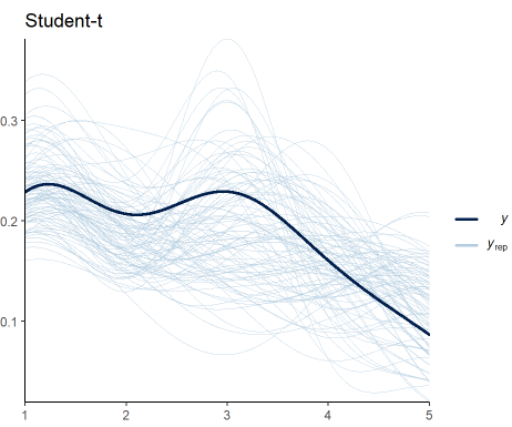
Figure 5 shows that my expectations were not met. Including the variance as a response in the model does not improve the fit to data. The trend is maintained, but the predictions still vary significantly. Nevertheless, this is another candidate we can consider to be our generative model.
We visualize the posterior distribution for this model:
describe_posterior(Ordinal_Fit2,
                   centrality = "mean",
                   dispersion = TRUE,
                   ci_method = "HDI",
                   test = "rope",
                   )
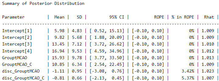
We can see a meaningful difference in the coefficients compared to the first model. The coefficient for “GrouptMCAO” increases from 8.6 to 15.9 and that for “GrouptMCAO_C” from 7 to 10.8. Undoubtedly, this model gives us a different picture. Otherwise, the variance term is presented under the names “disc_GrouptMCAO” and “disc_GrouptMCAO_C”. We can see that both variances are very different from our “sham” baseline.
Let’s plot the results:
Ordinal_CondEffects2 <-
  conditional_effects(Ordinal_Fit2, categorical = TRUE)

Ordinal_CondEffects2 <- plot(Ordinal_CondEffects2,
       plot = FALSE)[[1]]

Ordinal_CondEffects2 +
  Plot_theme +
  theme(legend.position = "bottom", legend.direction = "horizontal")
Contrary to what I expected, the model still predicts that sham animals have a small probability of scoring 1. What we have confirmed here is that this prediction is not based on the (false) assumption that all groups have the same variance. Nevertheless, it is still a logical prediction (not irrational) within this framework (ordinal regression) based on thresholds. If we go to Richard McElreath’s Statistical Rethinking (8) we find the same situation with monkeys pulling levers. Fitting a more constrained model will require the use of informative priors. Leave that for a future post. I know I made three promises here, but I will keep them.
In this model, the probabilities for the different outcomes in the tMCAO group shift slightly. However, given the high uncertainty, I will not change my conclusion about the performance of this group based on this model. For the tMCAO_C group, on the other hand, the predictions do not shift in a way that is readily apparent to the eye. Let’s conclude this blog post by comparing the two models.
We do the model comparison using the the loo package (9, 10) for leave-one-out cross validation. For an alternative approach using the WAIC criteria (11) I suggest you read this post also published by TDS Editors.
loo(Ordinal_Fit, Ordinal_Fit2)
Under this scheme, the models have very similar performance. In fact, the first model is slightly better for out-of-sample predictions. Accounting for variance did not help much in this particular case, where (perhaps) relying on informative priors can unlock the next step of scientific inference.
I would appreciate your comments or feedback letting me know if this journey was useful to you. If you want more quality content on data science and other topics, you might consider becoming a medium member.
In the future, you may find an updated version of this post on my GitHub site.
1.M. Bieber, J. Gronewold, A.-C. Scharf, M. K. Schuhmann, F. Langhauser, S. Hopp, S. Mencl, E. Geuss, J. Leinweber, J. Guthmann, T. R. Doeppner, C. Kleinschnitz, G. Stoll, P. Kraft, D. M. Hermann, Validity and Reliability of Neurological Scores in Mice Exposed to Middle Cerebral Artery Occlusion. Stroke. 50, 2875–2882 (2019).
2. P.-C. Bürkner, M. Vuorre, Ordinal Regression Models in Psychology: A Tutorial. Advances in Methods and Practices in Psychological Science. 2, 77–101 (2019).
3. G. Gigerenzer, Mindless statistics. The Journal of Socio-Economics. 33, 587–606 (2004).
4. P.-C. Bürkner, Brms: An r package for bayesian multilevel models using stan. 80 (2017), doi:10.18637/jss.v080.i01.
5. H. Wickham, M. Averick, J. Bryan, W. Chang, L. D. McGowan, R. François, G. Grolemund, A. Hayes, L. Henry, J. Hester, M. Kuhn, T. L. Pedersen, E. Miller, S. M. Bache, K. Müller, J. Ooms, D. Robinson, D. P. Seidel, V. Spinu, K. Takahashi, D. Vaughan, C. Wilke, K. Woo, H. Yutani, Welcome to the tidyverse. 4, 1686 (2019).
6. D. Makowski, M. S. Ben-Shachar, D. Lüdecke, bayestestR: Describing effects and their uncertainty, existence and significance within the bayesian framework. 4, 1541 (2019).
7. R. V. Lenth, Emmeans: Estimated marginal means, aka least-squares means (2023) (available at https://CRAN.R-project.org/package=emmeans).
8. R. McElreath, Statistical rethinking (Chapman; Hall/CRC, 2020; http://dx.doi.org/10.1201/9780429029608).
9. A. Vehtari, J. Gabry, M. Magnusson, Y. Yao, P.-C. Bürkner, T. Paananen, A. Gelman, Loo: Efficient leave-one-out cross-validation and WAIC for bayesian models (2022) (available at https://mc-stan.org/loo/).
10. A. Vehtari, A. Gelman, J. Gabry, Practical Bayesian model evaluation using leave-one-out cross-validation and WAIC. Statistics and Computing. 27, 1413–1432 (2016).
11. A. Gelman, J. Hwang, A. Vehtari, Understanding predictive information criteria for Bayesian models. Statistics and Computing. 24, 997–1016 (2013).
Avoiding abuse and misuse of T-test and ANOVA: Regression for categorical responses was originally published in Towards Data Science on Medium, where people are continuing the conversation by highlighting and responding to this story.
Originally appeared here:
Avoiding abuse and misuse of T-test and ANOVA: Regression for categorical responses
A quick introduction to cuDF, an NVIDIA framework for accelerating Pandas
Originally appeared here:
How to Empower Pandas with GPUs


This is how I used real estate data and powered them using OpenAI Large Language Model GPT3
Originally appeared here:
Hands-On Building a Virtual Property Consultant Using Artificial Intelligence


What if you were told there exists a new way to measure the relationship between two variables just like correlation except possibly better. More specifically, in 2020 a paper was published titled A New Coefficient of Correlation[1] introducing a new measure which equals 0 if and only if the two variables are independent, 1 if and only if one variable is a function of the other, and lastly has some nice theoretical properties allowing for hypothesis testing while practically making no assumptions about the data. Before we get into it, let us talk briefly about how more traditional correlation measures work.
There are few tools that exist to help understand data that are more commonly used (and misused) than the popular correlation coefficient. Formally known as Pearson’s r, the sample correlation coefficient taught in nearly every introductory statistics/business class is arguably the number one tool every data professional must be familiar with. The reasons for this are many, with one being it is both easy to use and interpret. As a reminder, the sample correlation coefficient measures the linear relationship between exactly two variables and can be calculated using the following formula.
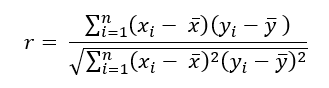
As a final reminder, this value can range from -1 to +1 with negative values implying an inverse linear relationship between the two variables being measured and a positive one implying the opposite. Notice the emphasis so far being placed on measuring linear relationships. Linear relationships can be understood as the shape of a relationship being somewhat traceable using a straight line.
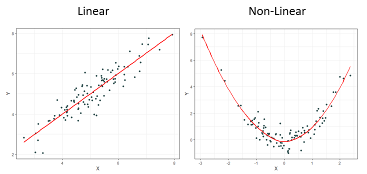
It should come as no surprise to most that it is rare to observe linear relationships in the real world. This is why other measures have been created over the decades such as Spearman’s ρ (rho) and Kendall’s τ (tau) to name a few. These newer measures are much better at identifying monotonic relationships and not just linear ones which makes them more robust since linear relationships are a specific type of monotonic relationship. Monotonic relationships can basically be understood as either always increasing or always decreasing.

Most of the time correlation is used, it is used to try and identify not necessarily a linear or monotonic relationship between two variables of interest, but instead identify if there exists any relationship. This creates problems, for if relationships are neither linear nor monotonic, these current measures do not work very well. Note how the plots below all display clearly strong relationships between two variables, but commonly used correlation techniques are only good at identifying monotonic ones.
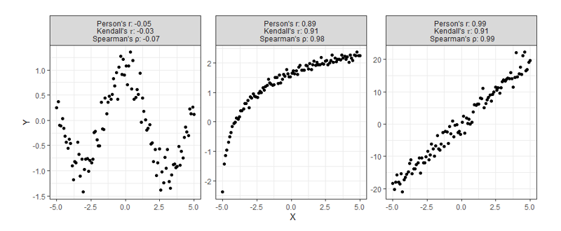
Despite having obvious shortcomings, these correlations are still being used to make many conclusions about all sorts of data. Is there any hope for identifying relationships that are even more complex than the ones shown above? Enter, the new coefficient ξ (pronounced “ksaai”).
One last note before moving on, a paper was published in 2022 titled Myths About Linear and Monotonic Associations[2] related to the issue of stating which popular measure of correlation is preferred for which type of data. Earlier, I suggested that Pearson’s r is most appropriate for linear measures while Spearman’s ρ and Kendall’s τ were better for monotonic data. While this rule is a popular belief and common practice amongst many data professionals, this paper makes a point to say that this is not necessarily the case, and that the opposite can in fact be true under certain circumstances.
Before introducing the formula, it is important to go over some needed prep-work. As we said earlier, correlation can be thought of as a way of measuring the relationship between two variables. Say we’re measuring the current correlation between X and Y. If a linear relationship does exist, it can be thought of as one that is mutually shared meaning the correlation between X and Y is always equal to the correlation between Y and X. With this new approach, however, we will no longer be measuring the linear relationship between X and Y, but instead our aim is to measure how much Y is a function of X. Understanding this subtle, but important distinction between traditional correlation techniques will make understanding the formulas much easier, for in general it is not necessarily the case anymore that ξ(X,Y) equals ξ(Y,X).
Sticking with the same train of thought, suppose we still wanted to measure how much Y is a function of X. Notice each data point is an ordered pair of both X and Y. First, we must sort the data as (X₍₁₎,Y₍₁₎),…,(X₍ₙ₎,Y₍ₙ₎) in a way that results in X₍₁₎ ≤ X₍₂₎≤ ⋯ ≤ X₍ₙ₎. Said clearly, we must sort the data according to X. We will then be able to create the variables r₁, r₂, … ,rₙ where rᵢ equals the rank of Y₍ᵢ₎. With these ranks now identified, we are ready to calculate.
There are two formulas used depending on the type of data you are working with. If ties in your data are impossible (or extremely unlikely), we have
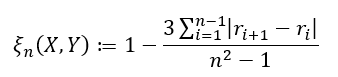
and if ties are allowed, we have
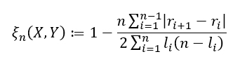
where lᵢ is defined as the number of j such that Y₍ ⱼ₎ ≥ Y₍ᵢ₎. One last important note for when ties are allowed. In addition to using the second formula, to obtain the best estimate possible it is important to randomly sort the observed ties in a way that one value is chosen to be ranked higher/lower over another so that (rᵢ₊₁ — rᵢ) is never equal to zero just as before. The variable lᵢ is then just the number of observations Y₍ᵢ₎ is actually greater than or equal to.
To not dive too much deeper into theory, it is also worth briefly pointing out this new correlation comes with some nice asymptotic theory behind it that makes it very easy to perform hypothesis testing without making any assumptions about the underlying distributions. This is because this method depends on the rank of the data, and not the values themselves making it a nonparametric statistic. If it is true that X and Y are independent and Y is continuous, then

What this means is that if you have a large enough sample size, then this correlation statistic approximately follows a normal distribution. This can be useful if you’d like to test the degree of independence between the two variables you are testing.
Along with the publishing of this new method, the R package XICOR was released containing a few relevant functions including one called xicor() which easily calculates the statistic ξ when X and Y vectors or matrices are provided as well as additional information like p-values for hypothesis testing. As with all articles I write, I will include original functions for R, Python, and Julia that you can simply copy and keep if you choose to. Here X and Y must either be a vector or an array, and for Python and Julia you may need to install the NumPy and Random package respectively.
## R Function ##
xicor <- function(X, Y, ties = TRUE){
  n <- length(X)
  r <- rank(Y[order(X)], ties.method = "random")
  set.seed(42)
  if(ties){
    l <- rank(Y[order(X)], ties.method = "max")
    return( 1 - n*sum( abs(r[-1] - r[-n]) ) / (2*sum(l*(n - l))) )
  } else {
    return( 1 - 3 * sum( abs(r[-1] - r[-n]) ) / (n^2 - 1) )
  }
}

## Python Function ##
from numpy import array, random, arrange

def xicor(X, Y, ties=True):
    random.seed(42)
    n = len(X)
    order = array([i[0] for i in sorted(enumerate(X), key=lambda x: x[1])])
    if ties:
        l = array([sum(y >= Y[order]) for y in Y[order]])
        r = l.copy()
        for j in range(n):
            if sum([r[j] == r[i] for i in range(n)]) > 1:
                tie_index = array([r[j] == r[i] for i in range(n)])
                r[tie_index] = random.choice(r[tie_index] - arange(0, sum([r[j] == r[i] for i in range(n)])), sum(tie_index), replace=False)
        return 1 - n*sum( abs(r[1:] - r[:n-1]) ) / (2*sum(l*(n - l)))
    else:
        r = array([sum(y >= Y[order]) for y in Y[order]])
        return 1 - 3 * sum( abs(r[1:] - r[:n-1]) ) / (n**2 - 1)

## Julia Function ##
import Random
function xicor(X::AbstractVector, Y::AbstractVector, ties::Bool=true)
    Random.seed!(42)
    n = length(X)
    if ties
        l = [sum(y .>= Y[sortperm(X)]) for y ∈ Y[sortperm(X)]]
        r = copy(l)
        for j ∈ 1:n
            if sum([r[j] == r[i] for i ∈ 1:n]) > 1
                tie_index = [r[j] == r[i] for i ∈ 1:n]
                r[tie_index] = Random.shuffle(r[tie_index] .- (0:sum([r[j] == r[i] for i ∈ 1:n])-1))
            end
        end
        return 1 - n*sum( abs.(r[2:end] - r[1:n-1]) ) / (2*sum(l.*(n .- l)))
    else
        r = [sum(y .>= Y[sortperm(X)]) for y ∈ Y[sortperm(X)]]
        return 1 - 3 * sum( abs.(r[2:end] - r[1:end-1]) ) / (n^2 - 1)
    end
end
For a first look at the possible benefits of using this new formula, let us compare the calculated correlation values of a few simulated examples that highlight the key differences between each correlation method.

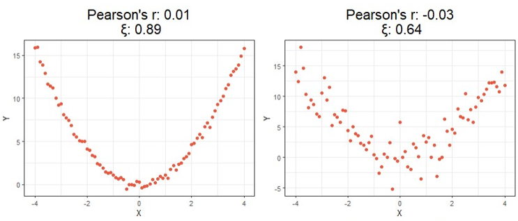
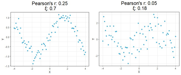
Starting at the top, we can see correlations using this new method no longer tell you the direction of the relationship since values can no longer be negative. As expected, however, this value is closer to 1 as the relationship strengthens and closer to 0 the more it weakens just like the aforementioned methods.
Moving on down is where things get exciting. It should be clear from the bottom four charts that this new approach is much more useful than traditional calculations at identifying significant relationships in general. Cases like these shown above are exactly the main motivation behind the research that led to this new formula since the second example shows Pearson’s r concludes there is no significant relationship between X and Y when there clearly exists a parabolic one, and the third example shows the same method concludes there’s a slight positive correlation when in reality the relationship appears to exhibit no upward trend.
Up to this point, we’ve only looked at simulated data. Let us now go over some visual results using this new correlation method with a real-world example. Suppose we want to measure the level of independence between brain signals and time.
The following data is a recording of brain activity measured in the form of BOLD signals using functional magnetic resonance imaging (fMRI) made available through the popular R package astsa. To provide more context, this dataset contains the average response observable in eight various brain locations in the cortex, thalamus, and cerebellum across five subjects. Each subject was exposed to periodic brushing of the hand for 32 seconds and then paused for 32 seconds resulting in a signal period of 64 seconds. Data was then recorded every 2 seconds for 256 seconds total (n = 128).
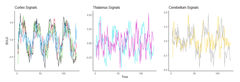
Suppose we wish to measure which of these three parts of the brain is most likely a function of time implying they are most involved when performing the prescribed stimulation. From the visual above, it appears that the Cortex signals are the least noisy, and one of the Thalamus’ signals are the noisiest, but let us quantify this using our new correlation statistic. The following table shows the correlation value of each of the eight measurements using the popular Pearson’s r and the new correlation ξ.
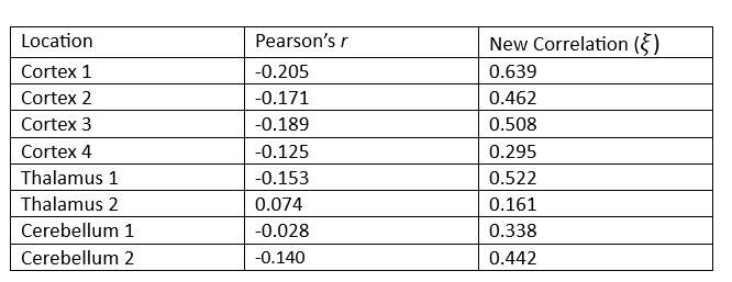
The table above reveals the common method for correlation consistently shows each of these relationships to be negative or approximately zero implying there is little to no observable relationship, and if there is one it exhibits a downward trend. This is clearly not the case since some of these wavelengths exhibit visibly strong relationships with time, and all of them appear to have no trend.
Furthermore, the new correlation values do a much better job identifying which location is least noisy, which is the main point of this analysis. The results show that parts of the Cortex are most notably being used during the period of stimulation since those correlation values are the highest on average, but there are also parts of the Thalamus that appear involved as well, a result not so easily detectable using the standard approach.
There is more that can be done to continue the analysis we started, such as perform an official hypothesis test of independence using the asymptotic theory presented earlier, but the purpose of this report was to simply introduce the new measure and showcase how simple these computations can be and how these results can be used. If you are interested in learning more about the pros and cons of this approach, I would encourage you to read the official publication introducing the method found in the references below.
This new approach is far from perfect, but it was created as a means of solving some of the most notable issues with the currently accepted approach. Since discovering it, I have been using it for my own personal research and it has proven very helpful.
Unless otherwise noted, all images, plots, and tables are by the author.
[1] S. Chatterjee, A New Coefficient of Correlation (2020), Journal of the American Statistical Association.
[2] E. Heuvel and Z. Zhan, Myths About Linear and Monotonic Associations (2022), The American Statistician.
A New Coefficient of Correlation was originally published in Towards Data Science on Medium, where people are continuing the conversation by highlighting and responding to this story.
Originally appeared here:
A New Coefficient of Correlation

Nikola Milosevic (Data Warrior)

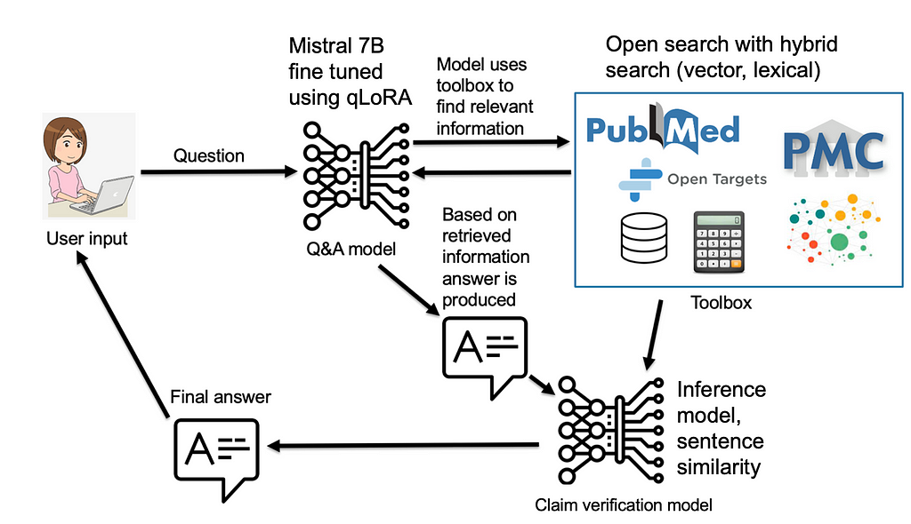
During the past year, I have been working on two projects dealing with hallucination detection of large language models and verifying claims produced by them. As with any research, especially one looking at verification of claims, it led to quite a bit of literature review, in which I have learned that a lot of authors, the task of verifying whether some claim is based on evidence from a reputable source (e.g. previous scientific publication, encyclopedia article, etc.) is often called fact-checking (examples of such publications include Google Deep Mind, University of Pennsylvania, University of Washington, Allen Institute for AI, OpenAI and others). Even datasets, such as SciFact, have factuality in the name.
I assume that calling some metric in large language models factuality goes back to the LaMDA paper by Google, which, published in February 2022, is to the best of my knowledge the first mention of such a metric in LLM. Before one could find occasional instances of fact-checking, like for example in a SciFact paper (from 2020), but LaMDA was the first mention related to LLMs. In the LaMDA paper, this metric was called factual grounding, which is a way better name than the later simplified versions, such as “factuality” or “faithfulness”. In this article, I would like to discuss why the name of the metric should be claim verification, and why I think names like faithfulness, factuality, and fact-checking are wrong from both practical and philosophical standpoints.
Let’s examine what is the base of the task. Given the claim that has been produced by a large language model, we are checking whether it is grounded in evidence from some source. This source can be an article from the literature, but it can be, also, some less formal source, such as encyclopedias, the internet, or any other kind of retrieved information source. Quite often, this task goes back to natural language entailment or natural language inference, where we find whether the claim can be derived from the evidence piece of text. However, there are other approaches, using textual similarity, or other large language models with various kinds of prompts. The task is always whether the generated claim is grounded in the evidence or knowledge we have of the world today. The task can be viewed similarly to generating a literature review part of an article or thesis, and verifying whether the referenced articles support the author’s claims. Of course, we are talking here about automating this task.
Now, what is the problem with naming this task fact-checking or measuring the factuality of the model?
From a philosophical standpoint, it is hard for us to know what the fact is. With all the best intentions, in their pursuit of truth, scientists often write in their publications things that may not be factual, and that will also easily pass peer review. I am here to emphasize, that people do their best effort, especially in scientific publishing, to be as factual as possible. However, that often fails. The publications may contain distorted, exaggerated, or misinterpreted information due to various factors, such as cultural biases, political agendas, or lack of reliable evidence. Often, science is just slowly and naturally moving toward facts by producing new evidence and information.
We had quite a few events in history, in which the common consensus in the field was set, in order to be shaken from its foundation. Think about for example Copernicus: Before Copernicus, most people believed that the Earth was the center of the universe and that the sun, the moon, and the planets revolved around it. This was the geocentric model, which was supported by the teachings of the Catholic Church and the ancient Greek philosopher Aristotle. However, Copernicus, a Polish astronomer and mathematician, proposed a radical alternative: the heliocentric model, which stated that the Earth and the other planets orbited the sun. He based his theory on mathematical calculations and observations of the celestial motions. His work was published in his book On the Revolutions of the Heavenly Spheres in 1543, shortly before his death. Although his theory faced strong opposition and criticism from the religious authorities and some of his contemporaries, it gradually gained acceptance and influence among other scientists, such as Galileo, Kepler, and Newton. The heliocentric model paved the way for the development of modern astronomy and physics and changed the perception of the Earth’s place in the cosmos.
A similar happened with Darwin. Before Darwin, most people believed that the living species were created by God and remained unchanged since their origin. This was the creationist view, which was based on the biblical account of Genesis and the natural theology of the British naturalist John Ray. However, Darwin, an English naturalist and geologist, proposed a radical alternative: the theory of evolution by natural selection, which stated that the living species descended from common ancestors and changed over time due to environmental pressures and the survival of the fittest. There are several more examples, such as Einstein’s relativity, gravity, Khan’s theory on scientific revolutions, and many others.
These events in history are called paradigm shifts, in which the base paradigm in certain fields was significantly shifted. Paradigm shifts may be fairly rare, however, we have as well many common beliefs and myths a lot of people believe, such as that the Great Wall of China can be seen from space, that Napoleon was short, or that Columbus discovered America, which can be found even in scientific articles or books written on the topics, despite them being untrue. People keep citing and referencing works containing this information and they still propagate. Therefore, checking whether the evidence in the referenced literature supports the claim is not a good enough proxy for factuality.
Providing references to the evidence we have for some claims is our best method for supporting the claim. Checking supporting evidence often requires also examining whether the reference is reputable, peer-reviewed, published in a reputable journal, year of publication, etc. Despite all these checks, the information may still be a victim of a paradigm shift or newly generated hypothesis and evidence for it and therefore incomplete and obsolete. But it is our best tool, and we should keep using it. Provided examples illustrate how verification of sources is not always fact-checking, but rather a way of approaching and evaluating claims based on the best available evidence and the most reasonable arguments at a given time and place. However, verification of sources does not imply that all claims are equally valid or that truth is relative or subjective. Verification of sources is a way of seeking and approximating the truth, not denying or relativizing it. Verification of sources acknowledges that truth is complex, multifaceted, and provisional, but also that truth is real, meaningful, and attainable.
Therefore, instead of using the term fact-checking, which suggests a binary and definitive judgment of true or false, we should use the term claim verification, which reflects a more nuanced and tentative assessment of supported or unsupported, credible or dubious, consistent or contradictory. Claim verification is not a final verdict, but a continuous inquiry, that invites us to question, challenge, and revise our beliefs and assumptions in light of new evidence, new sources, and new perspectives.
The right term for the task, in my opinion, is claim verification, as that is what we are doing, we are verifying whether the claim is grounded in the evidence from the referenced article, document, or source. There have been papers published naming the task claim verification (e.g. check this paper). So, I would like to try to call on authors working in this area, to avoid naming their metrics factuality, or fact-checking, but rather call it verifiability, claim verification, etc. I can assume that fact-checking from the marketing perspective looks better, but it is a bad name, not giving the proper treatment and credit to the pursuit of facts and truth in science, which is a much more complex task.
There is a big risk in that name from a practical point of view as well. In a situation where we “absolutely trust” some source to be “absolutely factual”, we lose the ability to critically examine this claim further. No one would have the courage or ability to do so. The core of science and critical thinking is that we examine everything in the pursuit of truth. On top of that, if AI in its current form, would measure factfulness and check facts only based on current knowledge and consensus, we are falling into the risk of halting progress and becoming especially averse to future paradigm shifts.
However, this risk is not only within sciences. The same argument of what is fact and excluding critical thinking from even whole educational systems is a common characteristic of authoritarian regimes. If we would less critically asses what is served to us as facts, we may fall victim to future authoritarians who would utilize it, and integrate their biases into what is considered “fact”. Therefore, let’s be careful of what we call fact, as in most cases it is a claim. A claim may be true based on our current understanding of the world and the universe, or not. Also, whether a claim is correct or not may change with the new evidence and new information that is discovered. One of the big challenges of AI systems, and especially knowledge representation, in my opinion, will be: how to represent knowledge that is our current understanding of the Universe and that will stay up-to-date over time.
Unless otherwise noted, all images are by the author.
Fact-checking vs claim verification was originally published in Towards Data Science on Medium, where people are continuing the conversation by highlighting and responding to this story.
Originally appeared here:
Fact-checking vs claim verification
Go Here to Read this Fast! Fact-checking vs claim verification


A breakdown of the the fields of statistics you should know for an entry-level data science role with useful resources
Originally appeared here:
What Statistics To Learn For Data Science
Go Here to Read this Fast! What Statistics To Learn For Data Science


New evaluations of RAG systems are published seemingly every day, and many of them focus on the retrieval stage of the framework. However, the generation aspect — how a model synthesizes and articulates this retrieved information — may hold equal if not greater significance in practice. Many use cases in production are not simply returning a fact from the context, but also require synthesizing the fact into a more complicated response.
We ran several experiments to evaluate and compare GPT-4, Claude 2.1 and Claude 3.0 Opus’s generation capabilities. This article details our research methodology, results, and model nuances encountered along the way as well as why this matters to people building with generative AI.
Everything needed to reproduce the results can be found in this GitHub repository.
While retrieval is responsible for identifying and retrieving the most pertinent information, it is the generation phase that takes this raw data and transforms it into a coherent, meaningful, and contextually appropriate response. The generative step is tasked with synthesizing the retrieved information, filling in gaps, and presenting it in a manner that is easily understandable and relevant to the user’s query.
In many real-world applications, the value of RAG systems lies not just in their ability to locate a specific fact or piece of information but also in their capacity to integrate and contextualize that information within a broader framework. The generation phase is what enables RAG systems to move beyond simple fact retrieval and deliver truly intelligent and adaptive responses.
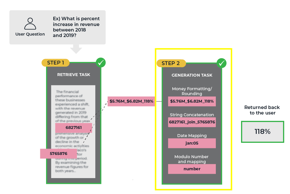
The initial test we ran involved generating a date string from two randomly retrieved numbers: one representing the month and the other the day. The models were tasked with:
For example, random numbers 4827143 and 17 would represent April 17th.
These numbers were placed at varying depths within contexts of varying length. The models initially had quite a difficult time with this task.
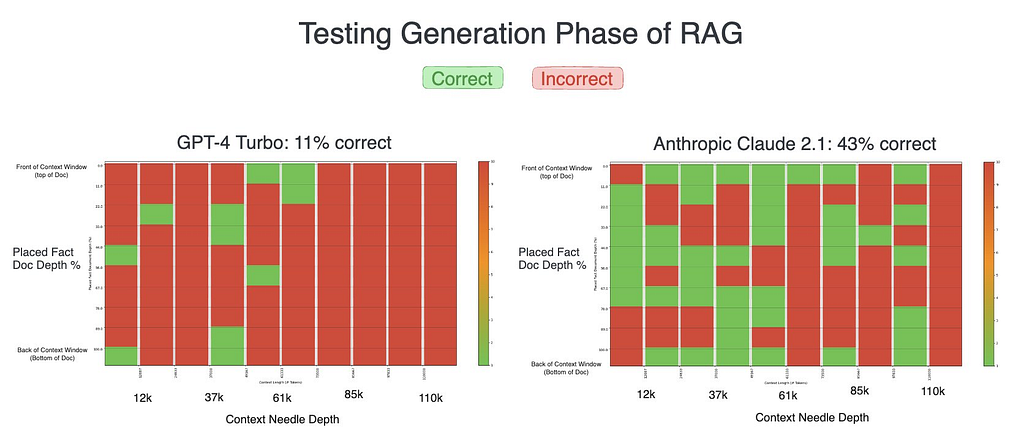
While neither model performed great, Claude 2.1 significantly outperformed GPT-4 in our initial test, almost quadrupling its success rate. It was here that Claude’s verbose nature — providing detailed, explanatory responses — seemed to give it a distinct advantage, resulting in more accurate outcomes compared to GPT-4’s initially concise replies.
Prompted by these unexpected results, we introduced a new variable to the experiment. We instructed GPT-4 to “explain yourself then answer the question,” a prompt that encouraged a more verbose response akin to Claude’s natural output. The impact of this minor adjustment was profound.
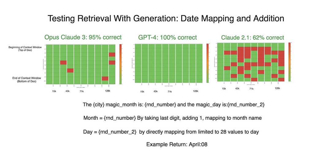
GPT-4’s performance improved dramatically, achieving flawless results in subsequent tests. Claude’s results also improved to a lesser extent.
This experiment not only highlights the differences in how language models approach generation tasks but also showcases the potential impact of prompt engineering on their performance. The verbosity that appeared to be Claude’s advantage turned out to be a replicable strategy for GPT-4, suggesting that the way a model processes and presents its reasoning can significantly influence its accuracy in generation tasks. Overall, including the seemingly minute “explain yourself” line to our prompt played a role in improving the models’ performance across all of our experiments.
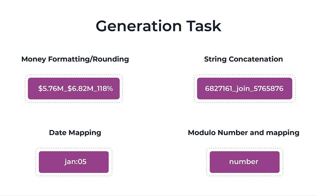
We conducted four more tests to assess prevailing models’ ability to synthesize and transform retrieved information into various formats:
Unsurprisingly, each model exhibited strong performance in string concatenation, reaffirming previous understanding that text manipulation is a fundamental strength of language models.
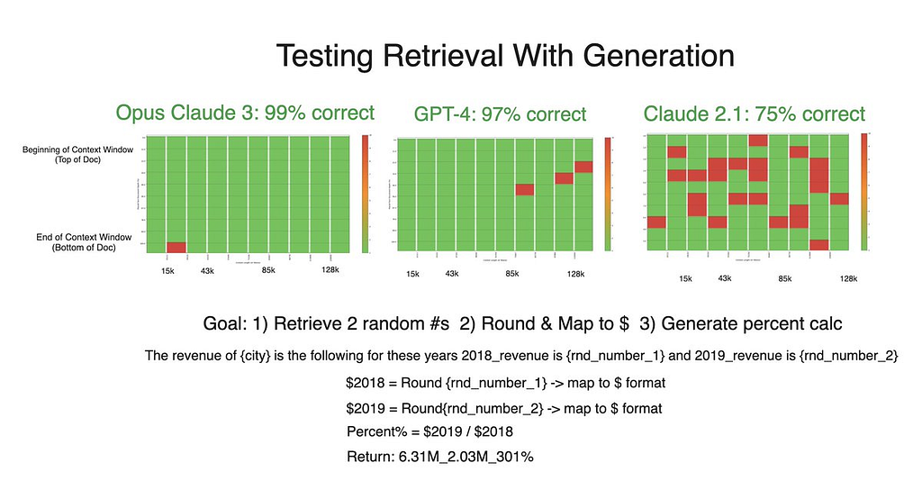
As for the money formatting test, Claude 3 and GPT-4 performed almost flawlessly. Claude 2.1’s performance was generally poorer overall. Accuracy did not vary considerably across token length, but was generally lower when the needle was closer to the beginning of the context window.
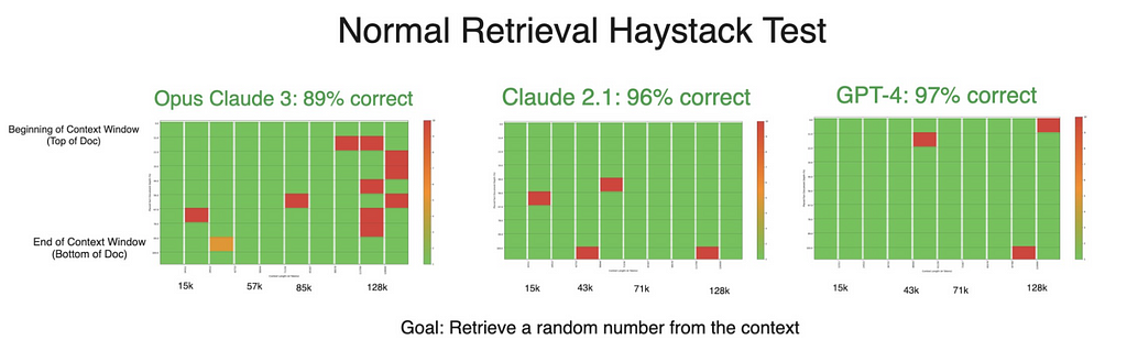
Despite stellar results in the generation tests, Claude 3’s accuracy declined in a retrieval-only experiment. Theoretically, simply retrieving numbers should be an easier task than manipulating them as well — making this decrease in performance surprising and an area where we’re planning further testing to examine. If anything, this counterintuitive dip only further confirms the notion that both retrieval and generation should be tested when developing with RAG.
By testing various generation tasks, we observed that while both models excel in menial tasks like string manipulation, their strengths and weaknesses become apparent in more complex scenarios. LLMs are still not great at math! Another key result was that the introduction of the “explain yourself” prompt notably enhanced GPT-4’s performance, underscoring the importance of how models are prompted and how they articulate their reasoning in achieving accurate results.
These findings have broader implications for the evaluation of LLMs. When comparing models like the verbose Claude and the initially less verbose GPT-4, it becomes evident that the evaluation criteria must extend beyond mere correctness. The verbosity of a model’s responses introduces a variable that can significantly influence their perceived performance. This nuance may suggest that future model evaluations should consider the average length of responses as a noted factor, providing a better understanding of a model’s capabilities and ensuring a fairer comparison.
Tips for Getting the Generation Part Right in Retrieval Augmented Generation was originally published in Towards Data Science on Medium, where people are continuing the conversation by highlighting and responding to this story.
Originally appeared here:
Tips for Getting the Generation Part Right in Retrieval Augmented Generation

Recently, I’ve come up with a particular issue when dealing with survival analysis: many models I fitted performed well in theory, with strong test metrics, but then failed to predict the true outcomes that were observed in practice. In this article, I want to discuss ways to better estimate the performance of our survival models, and a practical tip to help with extrapolation. Note: the main assumption here is that we count with several observations of our individuals over time (e.g., monthly observations for all the employees in a company).
The problem I was dealing with was the employee attrition case. I had information about several employees in a company, and I was interested in predicting which of them were most likely to leave in the future. If you want to explore the employee attrition topic further, make sure to check out this helpful article.
Many existing implementations on survival analysis start off with a dataset containing one observation per individual (patients in a health study, employees in the attrition case, clients in the client churn case, and so on). For these individuals we typically have two key variables: one signaling the event of interest (an employee quitting) and another measuring time (how long they’ve been with the company, up to either today or their departure). Together with these two variables, we then have explanatory variables with which we aim to predict the risk of each individual. These features can include the job role, age or compensation of the employee, for example.
Moving on, most implementations out there take a survival model (from simpler estimators such as Kaplan Meier to more complex ones like ensemble models or even neural networks), fit them over a train set and then evaluate over a test set. This train-test split is usually performed over the individual observations, generally making a stratified split.
In my case, I started with a dataset that followed several employees in a company monthly until December 2023 (in case the employee was still at the company), or until the month they left the company — the event date:
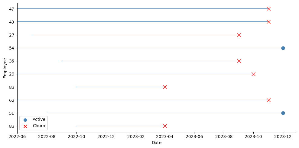
In order to adapt my data to the survival case, I took the last observation of each employee as shown in the picture above (the blue dots for active employees, and the red crosses for employees who left). At that point for each employee, I recorded whether the event had occurred at that date or not (if they were active or if they had left), their tenure in months at that time, and all their explanatory variables. I then performed a stratified train-test split over this data, like this:
import numpy as np
import pandas as pd
from sklearn.model_selection import train_test_split

# We load our dataset with several observations (record_date) per employee (employee_id)
# The event column indicates if the employee left on that given month (1) or if the employee was still active (0)
df = pd.read_csv(f'{FILE_NAME}.csv')

# Creating a label where positive events have tenure and negative events have negative tenure - required by Random Survival Forest
df_model['label'] = np.where(df_model['event'], df_model['tenure_in_months'], - df_model['tenure_in_months'])

df_train, df_test = train_test_split(df_model, test_size=0.2, stratify=df_model['event'], random_state=42)
After performing the split, I proceeded to fit a model. In this case, I chose to experiment with a Random Survival Forest using the scikit-survival library.
from sklearn.preprocessing import OrdinalEncoder
from sksurv.datasets import get_x_y
from sksurv.ensemble import RandomSurvivalForest

cat_features = [] # list of all the categorical features
features = [] # list of all the features (both categorical and numeric)

# Categorical Encoding
encoder = OrdinalEncoder(handle_unknown='use_encoded_value', unknown_value=-1)
encoder.fit(df_train[cat_features])

df_train[cat_features] = encoder.transform(df_train[cat_features])
df_test[cat_features] = encoder.transform(df_test[cat_features])

# X & y
X_train, y_train = get_x_y(df_train, attr_labels=['event','tenure_in_months'], pos_label=1)
X_test, y_test = get_x_y(df_test, attr_labels=['event','tenure_in_months'], pos_label=1)

# Fit the model
estimator = RandomSurvivalForest(random_state=RANDOM_STATE)
estimator.fit(X_train[features], y_train)

# Store predictions
y_pred = estimator.predict(X_test[features])
After a quick run using the default settings of the model, I was thrilled with the test metrics I saw. First of all, I was getting a concordance index above 0.90 in the test set. The concordance index is a measure of how well the model predicts the order of events: it reflects whether employees predicted to be at high risk were indeed the ones leaving the company first. An index of 1 corresponds to perfect prediction accuracy, while an index of 0.5 indicates a prediction no better than random chance.
I was particularly interested in seeing if the employees who left in the test set matched with the most risky employees according to the model. In the case of the Random Survival Forest, the model returns the risk scores of each observation. I took the percentage of employees who left the company in the test set, and used it to filter the most risky employees according to the model. The results were very solid, with the employees flagged with the most risk matching almost perfectly with the actual leavers, with an F1 score above 0.90 in the minority class.
from lifelines.utils import concordance_index
from sklearn.metrics import classification_report

# Concordance Index
ci_test = concordance_index(df_test['tenure_in_months'], -y_pred, df_test['event'])
print(f'Concordance index:{ci_test:0.5f}n')

# Match the most risky employees (according to the model) with the employees who left
q_test = 1 - df_test['event'].mean()

thr = np.quantile(y_pred, q_test)
risky_employees = (y_pred >= thr) * 1

print(classification_report(df_test['event'], risky_employees))
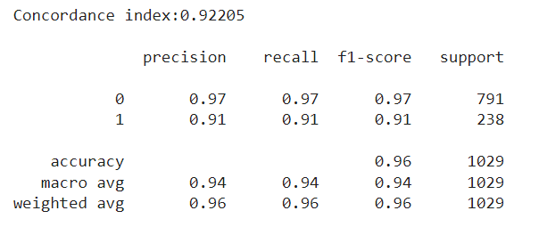
Getting +0.9 metrics on the first run should set off an alarm: was the model really able to predict whether an employee was going to stay or leave with such confidence? Imagine this: we submit our predictions saying which employees are most likely to leave. However, a couple months go by, and HR then reaches us worried, saying that the people who left during the last period, did not exactly match with our predictions, at least at the rate it was expected from our test metrics.
We have two main problems here: the first one is that our model isn’t extrapolating quite as well as we thought. The second one, and even worse, is that we weren’t able to measure this lack of performance. First, I’ll show a simple way we can estimate how well our model is truly extrapolating, and then I’ll talk about one potential reason it may be failing to do so, and how to mitigate it.
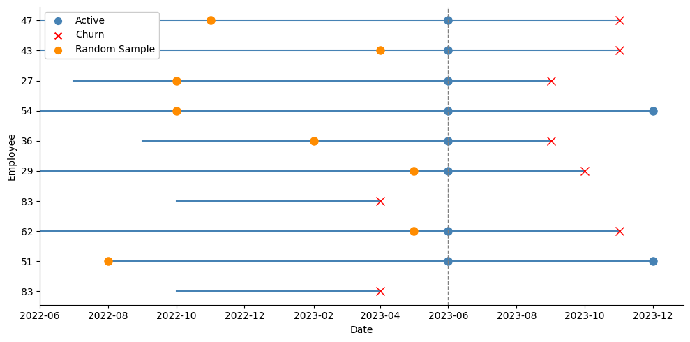
The key here is having access to panel data, that is, several records of our individuals over time, up until the time of event or the time the study ended (the date of our snapshot, in the case of employee attrition). Instead of discarding all this information and keeping only the last record of each employee, we could use it to create a test set that will better reflect how the model performs in the future. The idea is quite simple: suppose we have monthly records of our employees up until December 2023. We could move back, say, 6 months, and pretend we took the snapshot in June instead of December. Then, we would take the last observation for employees who left the company before June 2023 as positive events, and the June 2023 record of employees who survived beyond that date as negative events, even if we already know some of them eventually left afterwards. We are pretending we don’t know this yet.
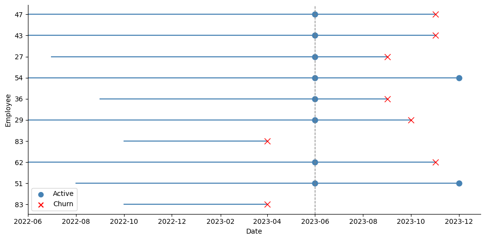
As the picture above shows, I take a snapshot in June, and all employees who were active at that time are taken as active. The test dataset takes all those active employees at June with their explanatory variables as they were on that date, and takes the latest tenure they achieved by December:
test_date = '2023-07-01'

# Selecting training data from records before the test date and taking the last observation per employee
df_train = df[df.record_date < test_date].reset_index(drop=True).copy()
df_train = df_train.groupby('employee_id').tail(1).reset_index(drop=True)
df_train['label'] = np.where(df_train['event'], df_train['tenure_in_months'], - df_train['tenure_in_months'])

# Preparing test data with records of active employees at the test date
df_test = df[(df.record_date == test_date) & (df['event']==0)].reset_index(drop=True).copy()
df_test = df_test.groupby('employee_id').tail(1).reset_index(drop=True)
df_test = df_test.drop(columns = ['tenure_in_months','event'])

# Fetching the last tenure and event status for employees in the test dataset
df_last_tenure = df[df.employee_id.isin(df_test.employee_id.unique())].reset_index(drop=True).copy()
df_last_tenure = df_last_tenure.groupby('employee_id').tail(1).reset_index(drop=True)

df_test = df_test.merge(df_last_tenure[['employee_id','tenure_in_months','event']], how='left')
df_test['label'] = np.where(df_test['event'], df_test['tenure_in_months'], - df_test['tenure_in_months'])
We fit our model again on this new train data, and once we finish we make our predictions for all employees who were active on June. We then compare these predictions to the actual outcome of July — December 2023 — this is our test set. If those employees we marked as having the most risk left during the semester, and those we marked as having the lowest risk didn’t leave, or left rather late in the period, then our model is extrapolating well. By shifting our analysis back in time and leaving the last period for evaluation, we can have a better understanding of how well our model is generalizing. Of course, we could take this one step further and perform some type of time-series cross validation. For example, we could iterate this process many times, each time moving 6 months back in time, and evaluating the model’s accuracy over several time frames.
After training our model once again, we now see a drastic decrease in performance. First of all, the concordance index is now around 0.5 — equivalent to that of a random predictor. Also, if we try to match the ‘n’ most risky employees according to the model with the ‘n’ employees who left in the test set, we see a very poor classification with a 0.15 F1 for the minority class:
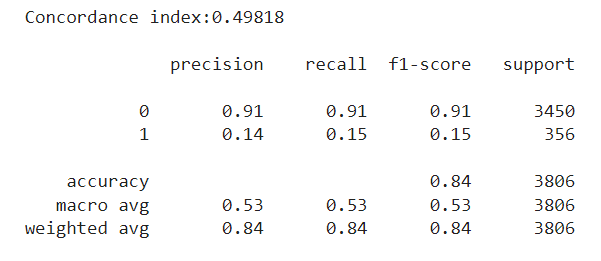
So clearly there is something wrong, but at least we are now able to detect it instead of being misled. The main takeaway here is that our model performs well with a traditional split, but doesn’t extrapolate when doing a time-based split. This is a clear sign that some time bias may be present. In short, time-dependent information is being leaked and our model is overfitting over it. This is common in cases like our employee attrition problem, when the dataset comes from a snapshot taken at some date.
The problem cuts down to this: all our positive observations (employees who left) belong to past dates, and all our negative observations (currently active employees) are all measured on the same date — today. If there is a single feature that reveals this to the model, then instead of predicting risk we will be predicting if an employee was recorded in December 2023 or before. This could be very subtle. For example, one feature we could be using is the engagement score of the employees. This feature could well show some seasonal patterns, and measuring it at the same time for active employees will surely introduce some bias in the model. Maybe in December, during the holiday season, this engagement score tends to decrease. The model will see a low score associated with all active employees, so it may learn to predict that whenever the engagement runs low, the churn risk also goes down, when in fact it should be the opposite!
By now, a simple yet quite effective solution for this problem should be clear: instead of taking the last observation for each active employee, we could just pick a random month from all their history within the company. This will strongly reduce the chances of the model picking on any temporal patterns that we do not want it to overfit on:
In the picture above we can see that we are now spanning a broader set of dates for the active employees. Instead of using their blue dots at June 2023, we take the random orange dots instead, and record their variables at the time, and the tenure they had so far in the company:
np.random.seed(0)

# Select training data before the test date
df_train = df[df.record_date < test_date].reset_index(drop=True).copy()

# Create an indicator for whether an employee eventually churns within the train set
df_train['indicator'] = df_train.groupby('employee_id').event.transform(max)

# Isolate records of employees who left, and store their last observation
churn = df_train[df_train.indicator==1].reset_index(drop=True).copy()
churn = churn.groupby('employee_id').tail(1).reset_index(drop=True)

# For employees who stayed, randomly pick one observation from their historic records
stay = df_train[df_train.indicator==0].reset_index(drop=True).copy()
stay = stay.groupby('employee_id').apply(lambda x: x.sample(1)).reset_index(drop=True)

# Combine churn and stay samples into the new training dataset
df_train = pd.concat([churn,stay], ignore_index=True).copy()
df_train['label'] = np.where(df_train['event'], df_train['tenure_in_months'], - df_train['tenure_in_months'])
del df_train['indicator']

# Prepare the test dataset similarly, using only the snapshot from the test date
df_test = df[(df.record_date == test_date) & (df.event==0)].reset_index(drop=True).copy()
df_test = df_test.groupby('employee_id').tail(1).reset_index(drop=True)
df_test = df_test.drop(columns = ['tenure_in_months','event'])

# Get the last known tenure and event status for employees in the test set
df_last_tenure = df[df.employee_id.isin(df_test.employee_id.unique())].reset_index(drop=True).copy()
df_last_tenure = df_last_tenure.groupby('employee_id').tail(1).reset_index(drop=True)

df_test = df_test.merge(df_last_tenure[['employee_id','tenure_in_months','event']], how='left')
df_test['label'] = np.where(df_test['event'], df_test['tenure_in_months'], - df_test['tenure_in_months'])
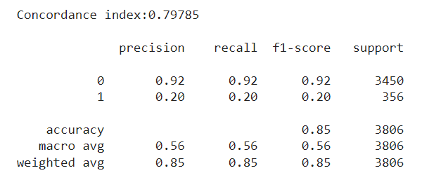
We then train our model once again, and evaluate it over the same test set we had before. We now see a concordance index of around 0.80. This isn’t the +0.90 we had earlier, but it definitely is a step up from the random-chance level of 0.5. Regarding our interest in classifying employees, we are still very far off the +0.9 F1 we had before, but we do see a slight increase compared to the previous approach, especially for the minority class.
To sum up, here are the main takeaways from our discussion:
I hope this walkthrough was useful. If you’ve been dealing with similar issues in survival analysis, I’d love to hear whether this approach works for you too. Thanks for reading!
Improving Generalization in Survival Models was originally published in Towards Data Science on Medium, where people are continuing the conversation by highlighting and responding to this story.
Originally appeared here:
Improving Generalization in Survival Models
Go Here to Read this Fast! Improving Generalization in Survival Models