
ChatGPT can take your data science game to the next level — if you know how to use it.
Originally appeared here:
In Defense of LLMs in Data Science: What ChatGPT Can and Can’t Do for Your Data Science Career
ChatGPT can take your data science game to the next level — if you know how to use it.
Originally appeared here:
In Defense of LLMs in Data Science: What ChatGPT Can and Can’t Do for Your Data Science Career


Originally appeared here:
AWS at NVIDIA GTC 2024: Accelerate innovation with generative AI on AWS
Go Here to Read this Fast! AWS at NVIDIA GTC 2024: Accelerate innovation with generative AI on AWS
Using synthetic data isn’t exactly a new practice: it’s been a productive approach for several years now, providing practitioners with the data they need for their projects in situations where real-world datasets prove inaccessible, unavailable, or limited from a copyright or approved-use perspective.
The recent rise of LLMs and AI-generated tools has transformed the synthetic-data scene, however, just as it has numerous other workflows for machine learning and data science professionals. This week, we’re presenting a collection of recent articles that cover the latest trends and possibilities you should be aware of, as well as the questions and considerations you should keep in mind if you decide to create your own toy dataset from scratch. Let’s dive in!

For more thought-provoking articles on other topics—from data career moves to multi-armed pendulums—we invite you to explore these recent standouts:
Thank you for supporting the work of our authors! If you’re feeling inspired to join their ranks, why not write your first post? We’d love to read it.
Until the next Variable,
TDS Team
How to Use Synthetic and Simulated Data Effectively was originally published in Towards Data Science on Medium, where people are continuing the conversation by highlighting and responding to this story.
Originally appeared here:
How to Use Synthetic and Simulated Data Effectively
Go Here to Read this Fast! How to Use Synthetic and Simulated Data Effectively
Leverage the power of the mPLUG-Owl document understanding model to ask questions about your documents
Originally appeared here:
Using a Multimodal Document ML Model to Query Your Documents
Go Here to Read this Fast! Using a Multimodal Document ML Model to Query Your Documents


The future of predictive analytics: Explore Moirai, Salesforce’s new foundation model for advanced time series forecasting
Originally appeared here:
Moirai: Time Series Foundation Models for Universal Forecasting
Go Here to Read this Fast! Moirai: Time Series Foundation Models for Universal Forecasting


A series of blog posts to share our perspectives on how to evaluate and improve your GenAI application pipelines
(written by Pasquale Antonante and Yi Zhang at Relari.ai)
The world of LLM app development is always on the move — new tricks, models, and apps pop up every week. As tech gets better, what users expect keeps ramping up. Staying ahead in this game is key to making sure it’s the one users keep coming back to.
The problem now becomes: how do you measure performance improvements? When you’re fiddling with prompts, tweaking the temperature, or switching up models, do you ever pause and think, “Will my users actually like this more?
In this post, we’ll walk through how in-app user feedback from earlier deployments (or internal human evaluation) can be instrumental in quickly shaping future versions of a product. We’ll discuss the limitations of traditional feedback mechanisms and introduce a new technique that allows AI developers to use feedback data directly in offline testing and iterations (before a new deployment), making the development cycle more adaptable and responsive to user preferences.
When developing LLM-based applications, we are often faced with a particular problem we want to address, e.g., a specific type of question has a low accuracy. As we experiment with tweaks in prompts, parameters, architecture, etc., we want to evaluate performance of the new pipeline, in particular whether users will like the new version(s) of your AI application. The most straightforward way is to A/B test each change with the end users and collect their feedback data such as thumbs up / down, score rating, or written comments, but practically it is challenging for a few reasons:
In the next section, we’ll introduce a novel approach that we’ve deployed to multiple customers to help them make the most out of their user feedback data in offline development.
In response to these challenges in collecting user feedback, we have developed a novel approach to simulate user feedback using a small sample of user (or internally labeled) feedback data. Specifically, we use metric ensembling and conformal prediction to learn user preferences and use them offline during the development phase. At its core, we learn how users weigh different criteria (e.g., tone, conciseness, etc) and leverage conformal prediction to provide predictions to quantify confidence. This method drastically accelerates LLM app development by providing a way to anticipate how users might react to new features or changes before they are fully implemented.
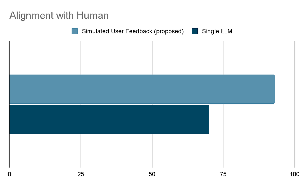
To evaluate its effectiveness, we compared this approach with the more conventional one of using a single LLM call that assesses different aspects of the response to make a judgment. To compare the two alternatives (the proposed approach vs. the single LLM call), we conducted an experiment using the Unified-Feedback dataset. We generated many potential …..We used Kendall’s tau, a measure of rank correlation, to compare the rankings produced by our user feedback simulation and the single LLM call approach against the ground truth established by human evaluations. This analysis allows us to assess not only the degree of agreement, but also the order of preference that each method predicts compared to the human rankings.
Our experiment revealed that the user feedback simulation has a correlation of 93% that significantly exceeded that of the single LLM call approach, which attains roughly 70% correlation. This indicates that, in terms of ranking , the simulated user feedback simulation provides a closer approximation to human judgment.
The reason why the simulated user feedback performs better is twofold:
While single LLM calls can identify major improvements in the pipeline, they fall short of detecting the more frequent, minor enhancements critical in mature pipelines. Simulated user feedback, however, exhibits a high correlation with human judgment, enabling the detection of these incremental advances.
As a side note, while we could have used the data to fine-tune an LLM, this has the typical drawback of requiring more data and not being as interpretable.
In the next section, we will walk through an example on how to create your simulated user feedback.
In this section we will show how we can use the open-source library continuous-eval to create simulated user feedback.
Consider a Q&A chatbot application. After deployment, users begin rating responses with thumbs up or down, indicating a need for performance enhancement. For this example we will use the example named correctness in continuous-eval:
dataset = Dataset(example_data_downloader("correctness"))

# Samples are annotated with "correct", "incorrect" or "refuse-to-answer"
# We remove the samples where the LLL refused to answer (i.e., said "I don't know")
dataset.filter(lambda x: x["annotation"] != "refuse-to-answer")
dataset.sample(300)  # Only for this example: randomly sample 300 examples
As we mentioned, we want to create some custom criteria. We leverage the LLMBasedCustomMetric class to define the Tone and Conciseness metrics. To do so we need to define the metric and provide a scoring rubric.
For the tone:
tone = LLMBasedCustomMetric(
    name="Tone",
    definition="The Tone/Content Issues metric evaluates the appropriateness and accuracy of the tone and content in responses to specific questions. It focuses on ensuring that the tone is professional and suitable for the context, and that the content accurately addresses the question without unnecessary deviations or inaccuracies. This metric is crucial for maintaining a professional image and ensuring clear, direct communication.",
    scoring_rubric="""Use the following rubric to assign a score to the answer based on its tone:
- Score 1: The response is inappropriate or inaccurate, with a tone that is either too informal, overly strong, or not suited to the professional context. The content may be irrelevant, incorrect, or fail to directly address the question posed.
- Score 2: The response is mostly appropriate and accurate but may contain minor tone or content issues. The tone is generally professional but may slip into informality or unnecessary strength in places. The content addresses the question but may include minor inaccuracies or unnecessary details.
- Score 3: The response is appropriate and accurate, with a tone that is professional and suited to the context. The content directly and correctly addresses the question without unnecessary deviations or inaccuracies.""",
    scoring_function=ScoringFunctions.Numeric(min_val=1, max_val=3),
    model_parameters={"temperature": 0},
)
while for conciseness:
conciseness = LLMBasedCustomMetric(
    name="Conciseness",
    definition="Conciseness in communication refers to the expression of ideas in a clear and straightforward manner, using the fewest possible words without sacrificing clarity or completeness of information. It involves eliminating redundancy, verbosity, and unnecessary details, focusing instead on delivering the essential message efficiently. ",
    scoring_rubric="""Use the following rubric to assign a score to the answer based on its conciseness:
- Score 1: The answer is overly verbose, containing a significant amount of unnecessary information, repetition, or redundant expressions that do not contribute to the understanding of the topic.
- Score 2: The answer includes some unnecessary details or slightly repetitive information, but the excess does not severely hinder understanding.
- Score 3: The answer is clear, direct, and to the point, with no unnecessary words, details, or repetition.""",
    scoring_function=ScoringFunctions.Numeric(min_val=1, max_val=3),
    model_parameters={"temperature": 0},
)
We use Tone and Conciseness together with more standard metrics, in particular we will consider the
The next step is to put all the metrics together and specify what field of the dataset should be used to compute the metrics. To do that we can use the SingleModulePipeline
pipeline = SingleModulePipeline(
    dataset=dataset,
    eval=[
        DeterministicAnswerCorrectness().use(
            answer=dataset.answer,
            ground_truth_answers=dataset.ground_truths,
        ),
        LLMBasedAnswerCorrectness().use(
            question=dataset.question,
            answer=dataset.answer,
            ground_truth_answers=dataset.ground_truths,
        ),
        LLMBasedAnswerRelevance().use(
            question=dataset.question, answer=dataset.answer
        ),
        LLMBasedStyleConsistency().use(
            answer=dataset.answer, ground_truth_answers=dataset.ground_truths
        ),
        FleschKincaidReadability().use(answer=dataset.answer),
        tone.use(
            question=dataset.question,
            answer=dataset.answer,
            ground_truth_answers=dataset.ground_truths,
        ),
        conciseness.use(
            question=dataset.question,
            answer=dataset.answer,
            ground_truth_answers=dataset.ground_truths,
        ),
    ],
)
and run all the metrics using the EvaluationManager
eval_manager = EvaluationManager(pipeline)
# The dataset already contains the model output so we just set the evaluation results
eval_manager.evaluation.results = dataset.data
eval_manager.run_metrics()  # Note: there is no progress bar, it might take a few minutes
The next step is to train simulated user feedback predictor
datasplit = DataSplit(
    X=eval_manager.metrics.to_pandas(),
    y=map(lambda x: 1 if x == "correct" else 0, dataset["annotation"]),
    split_ratios=SplitRatios(train=0.6, test=0.2, calibration=0.2),
)

# We use the train and calibration sets to train the classifier
predictor = EnsembleMetric(training=datasplit.train, calibration=datasplit.calibration)
This simulated user feedback predictor is able to correctly predict the human feedback in the test split 96.67% of the time.
We can leverage the proposed approach to better understand what is important to the user. Below is the learned importance of every metric by the simulated user feedback predictor.
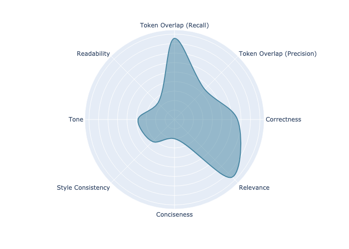
Looking at the plot, we see that Correctness (including token overlap, which is another measure for correctness) and Relevance to the question are the most important predictors of user preference. But the user also weighs tone and style consistency into the decision. At the same time, we can see that conciseness and readability are not as important. Reviewing this graph provides valuable insight into user preferences, giving a clear indication of what elements are essential and what can be adjusted if compromises need to be made.
Collecting user feedback is challenging, yet it is the most important information for developers of large language models (LLMs). By simulating user feedback during offline testing, we significantly reduces the time it takes for feedback to travel from the field back to developers, while maintaining positive user relationships.
In practice, our approach has proven to closely mirror actual human responses, outperforming traditional methods that rely on isolated LLM responses. This strategy allows for the incremental improvement of generative AI applications, fostering continuous refinement and greater congruence with what users expect.
—
Note: We will soon publish a research paper with more details on this methodology. Stay tuned!
How to make the most out of LLM production data: simulated user feedback was originally published in Towards Data Science on Medium, where people are continuing the conversation by highlighting and responding to this story.
Originally appeared here:
How to make the most out of LLM production data: simulated user feedback
Go Here to Read this Fast! How to make the most out of LLM production data: simulated user feedback


Some lessons I learned about quantifying qualitative thinking
Originally appeared here:
Why Human-Centred Approaches Lead to Better Algorithm Design
Go Here to Read this Fast! Why Human-Centred Approaches Lead to Better Algorithm Design

If you’re reading this article, you probably need no introduction to the advantages of deploying open-source models. Over the past couple of years, we have seen incredible growth in the both the quantity and quality of open source models.
Open-source models present an attractive solution, but what’s the next hurdle? Unlike using a model endpoint like OpenAI, where the model is a scalable black box behind the API, deploying your own open-source models introduces scaling challenges. It’s crucial to ensure that your model scales effectively with production traffic and maintains a seamless experience during traffic spikes. Additionally, it’s important to manage costs efficiently, so you only pay for what you use and avoid any financial surprises at the end of the month.
Interestingly, this sounds like a challenge that modern serverless architectures, like AWS Lambda, have already solved — a solution that have existed for almost a decade. However, when it comes to AI model deployment, this isn’t quite the case.
The limitations of serverless functions for AI deployments are multifaceted.
Next, let’s take a look at our scaling journey and the important lessons we have learned along the way.
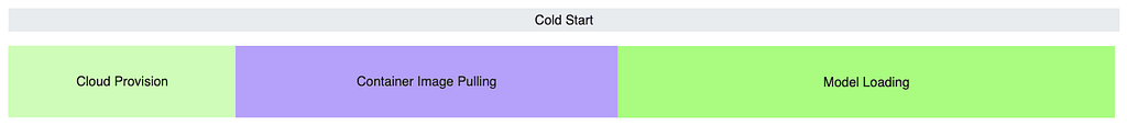
Before we could even begin to work on scaling, we have the notorious “cold start” problem. This issue presents itself in three different stages:
Each phase of the cold start issue demands specific strategies to minimize delays. In the following sections, we’ll explore each of them in more detail, sharing our strategies and solutions.
In contrast to the homogeneous environment of serverless CPUs, managing a diverse range of compute instance types is crucial when dealing with GPUs, each tailored for specific use cases. For instance, IO-bound LLMs require high GPU memory bandwidth and capacity, while generative models need more powerful GPU compute.
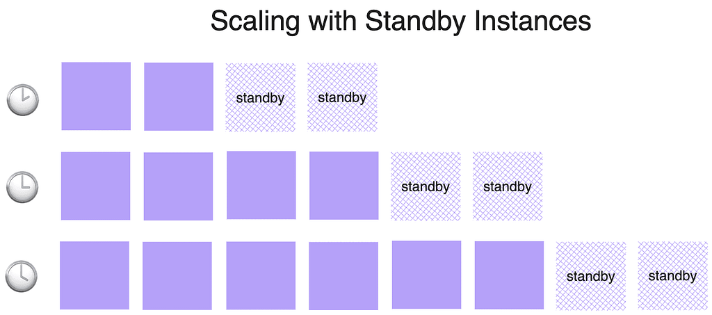
Ensuring availability during peak traffic by maintaining all GPU instance types could lead to prohibitively high costs. To avoid the financial strain of idle instances, we implemented a “standby instances” mechanism. Rather than preparing for the maximum potential load, we maintained a calculated number of standby instances that match the incremental scaling step sizes. For example, if we scale by two GPUs at a time, we need to have two standby instances ready. This allows us to quickly add resources to our serving fleet as demand surges, significantly reducing wait time, while keeping cost manageable.
In a multi-tenant environment, where multiple teams or, in our case, multiple organizations, share a common resource pool, we can achieve more efficient utilization rates. This shared environment allows us to balance varying resource demands, contributing to improved cost efficiency. However, managing multi-tenancy introduces challenges, such as enforcing quotas and ensuring network isolation, which can add complexity to the cluster.
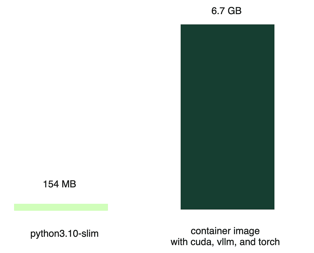
Serverless CPU workloads often use lightweight images, like the Python slim image (around 154 MB). In stark contrast, a container image built for serving an LLM can be much larger (6.7 GB); the bulk of this size comes from the various dependencies required to run the AI model.
Despite high-bandwidth networks advertised by cloud providers, the reality often falls short, with actual download speeds being a fraction of the promised rates.
Practically, a significant portion of the files were never used. One way is to optimize the container image itself, but that quickly proved to be unmanageable. Instead, we shifted our focus to an on-demand file pulling approach. Specifically, we first downloaded only the image metadata, with the actual remote files being fetched later as needed. In addition, we leveraged peer-to-peer networking within the cluster to dramatically increase pulling efficiency.
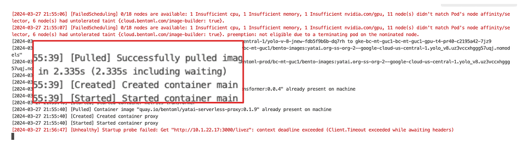
With these optimizations, we reduced the image pulling time from several minutes to mere seconds. However, we all know this measurement is “cheating” since the actual files are not pulled at this stage. The real file pulling occurs when the service runs. Therefore, it’s crucial to have a service framework that allows you to define behaviors at various lifecycle stages, such as initialization and serving. By doing all of the bootstrapping during initialization, we can ensure that all file dependencies are pulled. This way, when it comes to serving time, there are no delays caused by file pulling.
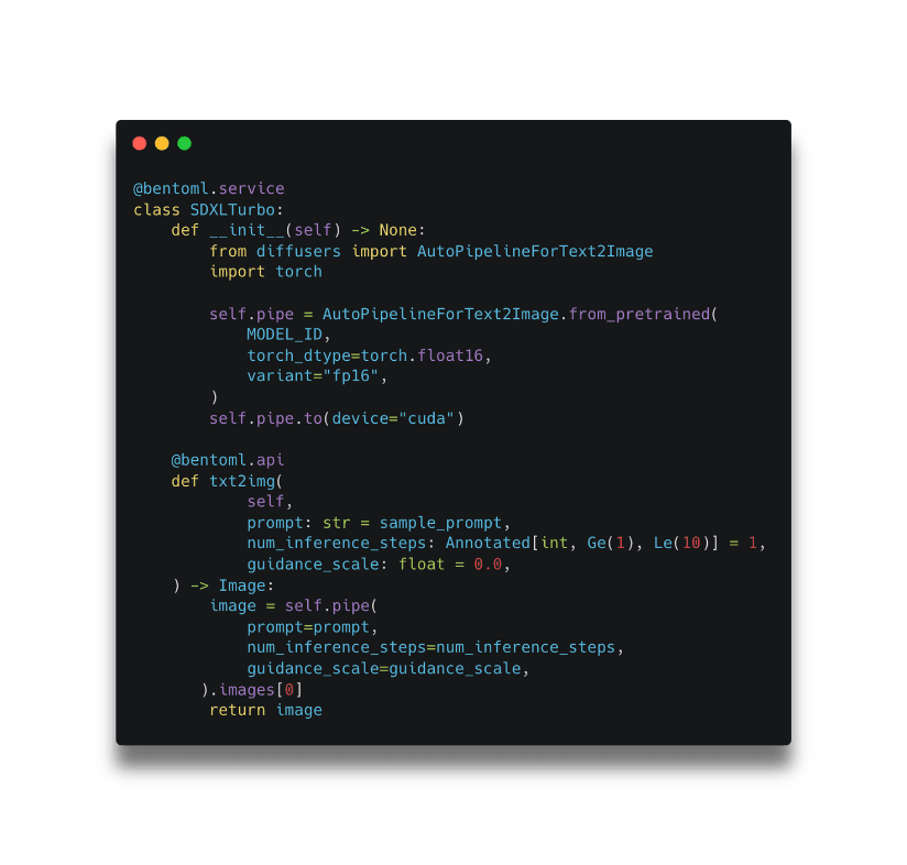
In the above example, model loading is done during the initialization lifecycle within __init__ and serving happens within the @bentoml.api named txt2img.
Initially, the most straightforward method for model loading was to fetch it directly from a remote store like Hugging Face. Using Content Delivery Networks (CDNs), NVMe SSDs, and shared memory, we could remove some of the bottlenecks. While this worked, it was far from optimal.
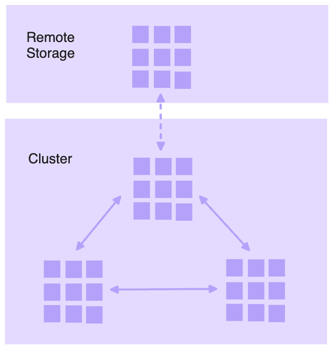
To improve this process, we considered using in-region network bandwidth. We seeded models in our distributed file systems and broke them into smaller chunks, allowing for parallel downloads. This drastically improved performance, but we still encountered cloud provider’s network bandwidth bottlenecks.
In response, we further optimized to leverage in-cluster network bandwidth by using peer-to-peer sharing and tapping into local caches. While the improvements were substantial, they added a layer of complexity to the process, which we need to abstract away from the developers.
Even with the above practices, we still suffer from a sequential bottleneck: the need to wait for each step to complete before proceeding with the next. Models had to be downloaded to persistent drive entirely before loading into CPU memory, and then into the GPU.
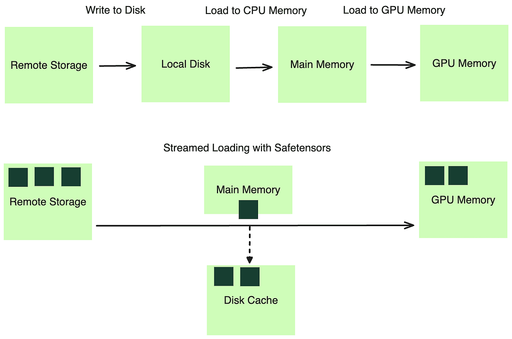
We turned to a stream-based method for loading model weights, using the distributed file cache system we had in place. This system allows programs to operate as if all files were logically available on disk. In reality, the required data is fetched on-demand from remote storage therefore bypassed disk writing. By leveraging a format like Safetensors, we can efficiently load the model weights into the main memory through memory mapping (mmap) before loading to the GPU memory in a streaming fashion.
Moreover, we adopted asynchronous writing to disk. By doing so, we created a faster-access cache layer on the local disk. Thus, new deployments with only code changes could bypass the slower remote storage fetch phase, reading the model weights from local cache directly.
To summarize, we managed to optimize the cold start time and we were happy with the results:
Next, we need to identify the most indicative signal for scaling AI model deployments on GPUs.
Initially, we considered CPU utilization. It’s straightforward and has an intuitive default threshold, such as 80%. However, the obvious drawback is that CPU metrics don’t capture GPU utilization. Additionally, the Global Interpreter Lock (GIL) in Python limits parallelism, preventing high CPU utilization on multi-core instances, making CPU utilization a less feasible metric.
We also explored GPU utilization as a more direct measure of our models’ workloads. However, we encountered an issue: the GPU utilization reported by tools like nvml didn’t accurately represent the actual utilization of the GPU. This metric samples kernel usage over a period of time, and a GPU is considered utilized if at least one kernel is executing. This aligns with our observation that better performance can often be achieved through improved batching, even though the GPU device was already reported as having high utilization.
Note: According to the NVIDIA documentation, utilization.gpu means “Percent of time over the past sample period during which one or more kernels was executing on the GPU. The sample period may be between 1 second and 1/6 second depending on the product”.
Resource-based metrics are inherently retrospective as they only reflect usage after the resources have been consumed. They’re also capped at 100%, which presents a problem: when scaling based on these metrics, the maximum ratio for adjustment is typically the current utilization over the desired threshold (see scaling formula below). This results in a conservative scale-up behavior that doesn’t necessarily match the actual demand of production traffic.
desiredReplicas = ceil[currentReplicas * ( currentMetricValue / desiredMetricValue )]
We turned to request-based metrics for more proactive signaling that are also not capped at a 100%.
QPS is a widely recognized metric for its simplicity. However, its application in generative AI, such as with LLMs, is still a question. QPS is not easy to configure and due to the variable cost per request, which depends on the number of tokens processed and generated, using QPS as a scaling metric can lead to inaccuracies.
Concurrency, on the other hand, has proven to be an ideal metric for reflecting the actual load on the system. It represents the number of active requests either queued or being processed. This metric:
For concurrency to work, we need the support from the service framework to automatically instrument concurrency as a metric and serve it as a scaling signal for the deployment platform. We must also establish right scaling policies to help against overzealous scale-up during a traffic spike or premature scale-down when traffic is sparse.
A another important mechanism we integrated with concurrency is the request queue. It acts as a buffer and an orchestrator, ensuring that incoming requests are handled efficiently and without overloading any single server replica.
In a scenario without a request queue, all incoming requests are dispatched directly to the server (6 requests in the image below). If multiple requests arrive simultaneously, and there’s only one active server replica, it becomes a bottleneck. The server tries to process each request in a first-come-first-serve manner, often leading to timeouts and a bad client experience.
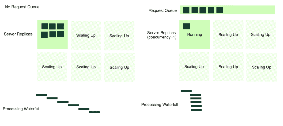
Conversely, with a request queue in place, the server consumes requests at an optimal rate, processing at a rate based on the concurrency defined for the service. When additional server replicas scale up, they too begin to pull from the queue. This mechanism prevents any single server from becoming overwhelmed and allows for a smoother, more manageable distribution of requests across the available infrastructure.
Our journey in exploring AI model scaling solutions has been an adventure, which has led us to ultimately create the scaling experience on BentoCloud — a platform that encapsulates all our learnings.
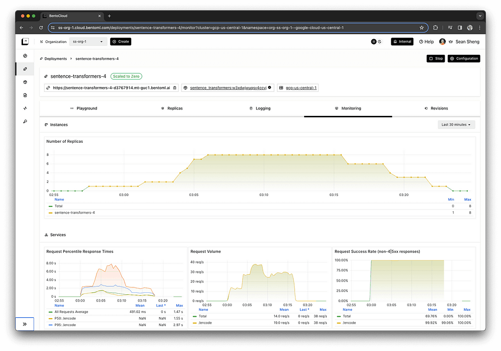
To avoid the impression of a promotion, we’ll illustrate our point with a picture that’s worth a thousand words. The monitoring dashboard below demonstrates the correlation between incoming requests and the scaling up of server instances.
Equally important to scaling up is the ability to scale down. As the requests waned to zero, the deployment reduced the number of active instances accordingly. This ability ensures that no unnecessary costs are incurred for unused resources, aligning expenditure with actual usage.
We hope the takeaway is that scaling for model deployments should be considered an important aspect of production applications. Unlike scaling CPU workloads, scaling model deployments on GPUs presents unique challenges, including cold start times, configuring scaling metrics, and orchestrating requests. When evaluating deployment platforms, their solutions to these challenges should be thoroughly assessed.
Scaling AI Models Like You Mean It was originally published in Towards Data Science on Medium, where people are continuing the conversation by highlighting and responding to this story.
Originally appeared here:
Scaling AI Models Like You Mean It
Go Here to Read this Fast! Scaling AI Models Like You Mean It


A Huge thanks to Martim Chaves who co-authored this post and developed the example scripts.
In our previous post we took a high level view of how to train a machine learning model in Microsoft Fabric. In this post we wanted to dive deeper into the process of feature engineering.
Feature engineering is a crucial part of the development lifecycle for any Machine Learning (ML) systems. It is a step in the development cycle where raw data is processed to better represent its underlying structure and provide additional information that enhance our ML models. Feature engineering is both an art and a science. Even though there are specific steps that we can take to create good features, sometimes, it is only through experimentation that good results are achieved. Good features are crucial in guaranteeing a good system performance.
As datasets grow exponentially, traditional feature engineering may struggle with the size of very large datasets. This is where PySpark can help — as it is a scalable and efficient processing platform for massive datasets. A great thing about Fabric is that it makes using PySpark easy!
In this post, we’ll be going over:
By the end of this post, hopefully you’ll feel comfortable carrying out feature engineering with PySpark in Fabric. Let’s get started!
Spark is a distributed computing system that allows for the processing of large datasets with speed and efficiency across a cluster of machines. It is built around the concept of a Resilient Distributed Dataset (RDD), which is a fault-tolerant collection of elements that can be operated on in parallel. RDDs are the fundamental data structure of Spark, and they allow for the distribution of data across a cluster of machines.
PySpark is the Python API for Spark. It allows for the creation of Spark DataFrames, which are similar to Pandas DataFrames, but with the added benefit of being distributed across a cluster of machines. PySpark DataFrames are the core data structure in PySpark, and they allow for the manipulation of large datasets in a distributed manner.
At the core of PySpark is the SparkSession object, which is what fundamentally interacts with Spark. This SparkSession is what allows for the creation of DataFrames, and other functionalities. Note that, when running a Notebook in Fabric, a SparkSession is automatically created for you, so you don’t have to worry about that.
Having a rough idea of how PySpark works, let’s get to the basics.
Although Spark DataFrames may remind us of Pandas DataFrames due to their similarities, the syntax when using PySpark can be a bit different. In this section, we’ll go over some of the basics of PySpark, such as reading data, combining DataFrames, selecting columns, grouping data, joining DataFrames, and using functions.
The data we are looking at is from the 2024 US college basketball tournaments, which was obtained from the on-going March Machine Learning Mania 2024 Kaggle competition, the details of which can be found here, and is licensed under CC BY 4.0 [1]
As mentioned in the previous post of this series, the first step is usually to create a Lakehouse and upload some data. Then, when creating a Notebook, we can attach it to the created Lakehouse, and we’ll have access to the data stored there.
PySpark Dataframes can read various data formats, such as CSV, JSON, Parquet, and others. Our data is stored in CSV format, so we’ll be using that, like in the following code snippet:
# Read women's data
w_data = (
    spark.read.option("header", True)
    .option("inferSchema", True)
    .csv(f"Files/WNCAATourneyDetailedResults.csv")
    .cache()
)
In this code snippet, we’re reading the detailed results data set of the final women’s basketball college tournament matches. Note that the “header” option being true means that the names of the columns will be derived from the first row of the CSV file. The inferSchema option tells Spark to guess the data types of the columns – otherwise they would all be read as strings. .cache() is used to keep the DataFrame in memory.
If you’re coming from Pandas, you may be wondering what the equivalent of df.head() is for PySpark – it’s df.show(5). The default for .show() is the top 20 rows, hence the need to specifically select 5.
Combining DataFrames can be done in multiple ways. The first we will look at is a union, where the columns are the same for both DataFrames:
# Read women's data
...

# Read men's data
m_data = (
    spark.read.option("header", True)
    .option("inferSchema", True)
    .csv(f"Files/MNCAATourneyDetailedResults.csv")
    .cache()
)

# Combine (union) the DataFrames
combined_results = m_data.unionByName(w_data)
Here, unionByName joins the two DataFrames by matching the names of the columns. Since both the women’s and the men’s detailed match results have the same columns, this is a good approach. Alternatively, there’s also union, which combines two DataFrames, matching column positions.
Selecting columns from a DataFrame in PySpark can be done using the .select() method. We just have to indicate the name or names of the columns that are relevant as a parameter.
Here’s the output for w_scores.show(5):
# Selecting a single column
w_scores = w_data.select("WScore")

# Selecting multiple columns
teamid_w_scores = w_data.select("WTeamID", "WScore")
```

Here's the output for `w_scores.show(5)`:
```
+------+
|Season|
+------+
|  2010|
|  2010|
|  2010|
|  2010|
|  2010|
+------+
only showing top 5 rows
The columns can also be renamed when being selected using the .alias() method:
winners = w_data.select(
    w_data.WTeamID.alias("TeamID"),
    w_data.WScore.alias("Score")
)
Grouping allows us to carry out certain operations for the groups that exist within the data and is usually combined with a aggregation functions. We can use .groupBy() for this:
# Grouping and aggregating
winners_average_scores = winners.groupBy("TeamID").avg("Score")
In this example, we are grouping by “TeamID”, meaning we’re considering the groups of rows that have a distinct value for “TeamID”. For each of those groups, we’re calculating the average of the “Score”. This way, we get the average score for each team.
Here’s the output of winners_average_scores.show(5), showing the average score of each team:
+------+-----------------+
|TeamID|       avg(Score)|
+------+-----------------+
|  3125|             68.5|
|  3345|             74.2|
|  3346|79.66666666666667|
|  3376|73.58333333333333|
|  3107|             61.0|
+------+-----------------+
Joining two DataFrames can be done using the .join() method. Joining is essentially extending the DataFrame by adding the columns of one DataFrame to another.
# Joining on Season and TeamID
final_df = matches_df.join(stats_df, on=['Season', 'TeamID'], how='left')
In this example, both stats_df and matches_df were using Season and TeamID as unique identifiers for each row. Besides Season and TeamID, stats_df has other columns, such as statistics for each team during each season, whereas matches_df has information about the matches, such as date and location. This operation allows us to add those interesting statistics to the matches information!
There are several functions that PySpark provides that help us transform DataFrames. You can find the full list here.
Here’s an example of a simple function:
from pyspark.sql import functions as F

w_data = w_data.withColumn("HighScore", F.when(F.col("Score") > 80, "Yes").otherwise("No"))
In the code snippet above, a “HighScore” column is created when the score is higher than 80. For each row in the “Score” column (indicated by the .col() function), the value “Yes” is chosen for the “HighScore” column if the “Score” value is larger than 80, determined by the .when() function. .otherwise(), the value chosen is “No”.
Now that we have a basic understanding of PySpark and how it can be used, let’s go over how the regular season statistics features were created. These features were then used as inputs into our machine learning model to try to predict the outcome of the final tournament games.
The starting point was a DataFrame, regular_data, that contained match by match statistics for the regular seasons, which is the United States College Basketball Season that happens from November to March each year.
Each row in this DataFrame contained the season, the day the match was held, the ID of team 1, the ID of team 2, and other information such as the location of the match. Importantly, it also contained statistics for each team for that specific match, such as “T1_FGM”, meaning the Field Goals Made (FGM) for team 1, or “T2_OR”, meaning the Offensive Rebounds (OR) of team 2.
The first step was selecting which columns would be used. These were columns that strictly contained in-game statistics.
# Columns that we'll want to get statistics from
boxscore_cols = [
    'T1_FGM', 'T1_FGA', 'T1_FGM3', 'T1_FGA3', 'T1_OR', 'T1_DR', 'T1_Ast', 'T1_Stl', 'T1_PF',
    'T2_FGM', 'T2_FGA', 'T2_FGM3', 'T2_FGA3', 'T2_OR', 'T2_DR', 'T2_Ast', 'T2_Stl', 'T2_PF'
]
If you’re interested, here’s what each statistic’s code means:
From there, a dictionary of aggregation expressions was created. Basically, for each column name in the previous list of columns, a function was stored that would calculate the mean of the column, and rename it, by adding a suffix, “mean”.
from pyspark.sql import functions as F
from pyspark.sql.functions import col  # select a column

agg_exprs = {col: F.mean(col).alias(col + 'mean') for col in boxscore_cols}
Then, the data was grouped by “Season” and “T1_TeamID”, and the aggregation functions of the previously created dictionary were used as the argument for .agg().
season_statistics = regular_data.groupBy(["Season", "T1_TeamID"]).agg(*agg_exprs.values())
Note that the grouping was done by season and the ID of team 1 — this means that “T2_FGAmean”, for example, will actually be the mean of the Field Goals Attempted made by the opponents of T1, not necessarily of a specific team. So, we actually need to rename the columns that are something like “T2_FGAmean” to something like “T1_opponent_FGAmean”.
# Rename columns for T1
for col in boxscore_cols:
    season_statistics = season_statistics.withColumnRenamed(col + 'mean', 'T1_' + col[3:] + 'mean') if 'T1_' in col
        else season_statistics.withColumnRenamed(col + 'mean', 'T1_opponent_' + col[3:] + 'mean')
At this point, it’s important to mention that the regular_data DataFrame actually has two rows per each match that occurred. This is so that both teams can be “T1” and “T2”, for each match. This little “trick” is what makes these statistics useful.
Note that we “only” have the statistics for “T1”. We “need” the statistics for “T2” as well — “need” in quotations because there are no new statistics being calculated. We just need the same data, but with the columns having different names, so that for a match with “T1” and “T2”, we have statistics for both T1 and T2. So, we created a mirror DataFrame, where, instead of “T1…mean” and “T1_opponent_…mean”, we have “T2…mean” and “T2_opponent_…mean”. This is important because, later on, when we’re joining these regular season statistics to tournament matches, we’ll be able to have statistics for both team 1 and team 2.
season_statistics_T2 = season_statistics.select(
    *[F.col(col).alias(col.replace('T1_opponent_', 'T2_opponent_').replace('T1_', 'T2_')) if col not in ['Season'] else F.col(col) for col in season_statistics.columns]
)
Now, there are two DataFrames, with season statistics for “both” T1 and T2. Since the final DataFrame will contain the “Season”, the “T1TeamID” and the “T2TeamID”, we can join these newly created features with a join!
tourney_df = tourney_df.join(season_statistics, on=['Season', 'T1_TeamID'], how='left')
tourney_df = tourney_df.join(season_statistics_T2, on=['Season', 'T2_TeamID'], how='left')
First created by Arpad Elo, Elo is a rating system for zero-sum games (games where one player wins and the other loses), like basketball. With the Elo rating system, each team has an Elo rating, a value that generally conveys the team’s quality. At first, every team has the same Elo, and whenever they win, their Elo increases, and when they lose, their Elo decreases. A key characteristic of this system is that this value increases more with a win against a strong opponent than with a win against a weak opponent. Thus, it can be a very useful feature to have!
We wanted to capture the Elo rating of a team at the end of the regular season, and use that as feature for the tournament. To do this, we calculated the Elo for each team on a per match basis. To calculate Elo for this feature, we found it more straightforward to use Pandas.
Central to Elo is calculating the expected score for each team. It can be described in code like so:
# Function to calculate expected score
def expected_score(ra, rb):
    # ra = rating (Elo) team A
    # rb = rating (Elo) team B
    # Elo function
    return 1 / (1 + 10 ** ((rb - ra) / 400))
Considering a team A and a team B, this function computes the expected score of team A against team B.
For each match, we would update the teams’ Elos. Note that the location of the match also played a part — winning at home was considered less impressive than winning away.
# Function to update Elo ratings, keeping T1 and T2 terminology
def update_elo(t1_elo, t2_elo, location, T1_Score, T2_Score):
    expected_t1 = expected_score(t1_elo, t2_elo)
    expected_t2 = expected_score(t2_elo, t1_elo)

    actual_t1 = 1 if T1_Score > T2_Score else 0
    actual_t2 = 1 - actual_t1

    # Determine K based on game location
    # The larger the K, the bigger the impact
    # team1 winning at home (location=1) less impressive than winning away (location = -1)
    if actual_t1 == 1:  # team1 won
        if location == 1:
            k = 20
        elif location == 0:
            k = 30
        else:  # location = -1
            k = 40
    else:  # team2 won
        if location == 1:
            k = 40
        elif location == 0:
            k = 30
        else:  # location = -1
            k = 20

    new_t1_elo = t1_elo + k * (actual_t1 - expected_t1)
    new_t2_elo = t2_elo + k * (actual_t2 - expected_t2)

    return new_t1_elo, new_t2_elo
To apply the Elo rating system, we iterated through each season’s matches, initializing teams with a base rating and updating their ratings match by match. The final Elo available for each team in each season will, hopefully, be a good descriptor of the team’s quality.
def calculate_elo_through_seasons(regular_data):

    # For this feature, using Pandas
    regular_data = regular_data.toPandas()

    # Set value of initial elo
    initial_elo = 1500

    # DataFrame to collect final Elo ratings
    final_elo_list = []

    for season in sorted(regular_data['Season'].unique()):
        print(f"Season: {season}")
        # Initialize elo ratings dictionary
        elo_ratings = {}

        print(f"Processing Season: {season}")
        # Get the teams that played in the season
        season_teams = set(regular_data[regular_data['Season'] == season]['T1_TeamID']).union(set(regular_data[regular_data['Season'] == season]['T2_TeamID']))

        # Initialize season teams' Elo ratings
        for team in season_teams:
            if (season, team) not in elo_ratings:
                elo_ratings[(season, team)] = initial_elo

        # Update Elo ratings per game
        season_games = regular_data[regular_data['Season'] == season]
        for _, row in season_games.iterrows():
            t1_elo = elo_ratings[(season, row['T1_TeamID'])]
            t2_elo = elo_ratings[(season, row['T2_TeamID'])]

            new_t1_elo, new_t2_elo = update_elo(t1_elo, t2_elo, row['location'], row['T1_Score'], row['T2_Score'])

            # Only keep the last season rating
            elo_ratings[(season, row['T1_TeamID'])] = new_t1_elo
            elo_ratings[(season, row['T2_TeamID'])] = new_t2_elo

        # Collect final Elo ratings for the season
        for team in season_teams:
            final_elo_list.append({'Season': season, 'TeamID': team, 'Elo': elo_ratings[(season, team)]})

    # Convert list to DataFrame
    final_elo_df = pd.DataFrame(final_elo_list)

    # Separate DataFrames for T1 and T2
    final_elo_t1_df = final_elo_df.copy().rename(columns={'TeamID': 'T1_TeamID', 'Elo': 'T1_Elo'})
    final_elo_t2_df = final_elo_df.copy().rename(columns={'TeamID': 'T2_TeamID', 'Elo': 'T2_Elo'})

    # Convert the pandas DataFrames back to Spark DataFrames
    final_elo_t1_df = spark.createDataFrame(final_elo_t1_df)
    final_elo_t2_df = spark.createDataFrame(final_elo_t2_df)

    return final_elo_t1_df, final_elo_t2_df
Ideally, we wouldn’t calculate Elo changes on a match-by-match basis to determine each team’s final Elo for the season. However, we couldn’t come up with a better approach. Do you have any ideas? If so, let us know!
The feature engineering steps demonstrated show how we can transform raw data — regular season statistics — into valuable information with predictive power. It is reasonable to assume that a team’s performance during the regular season is indicative of its potential performance in the final tournaments. By calculating the mean of observed match-by-match statistics for both the teams and their opponents, along with each team’s Elo rating in their final match, we were able to create a dataset suitable for modelling. Then, models were trained to predict the outcome of tournament matches using these features, among others developed in a similar way. With these models, we only need the two team IDs to look up the mean of their regular season statistics and their Elos to feed into the model and predict a score!
In this post, we looked at some of the theory behind Spark and PySpark, how that can be applied, and a concrete practical example. We explored how feature engineering can be done in the case of sports data, creating regular season statistics to use as features for final tournament games. Hopefully you’ve found this interesting and helpful — happy feature engineering!
The full source code for this post and others in the series can be found here.
Originally published at https://nobledynamic.com on April 8, 2024.
[1] Jeff Sonas, Ryan Holbrook, Addison Howard, Anju Kandru. (2024). March Machine Learning Mania 2024. Kaggle. https://kaggle.com/competitions/march-machine-learning-mania-2024
Feature Engineering with Microsoft Fabric and PySpark was originally published in Towards Data Science on Medium, where people are continuing the conversation by highlighting and responding to this story.
Originally appeared here:
Feature Engineering with Microsoft Fabric and PySpark
Go Here to Read this Fast! Feature Engineering with Microsoft Fabric and PySpark

Originally appeared here:
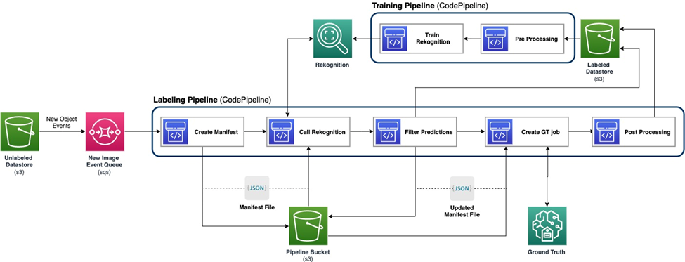
Build an active learning pipeline for automatic annotation of images with AWS services