How to implement a caching mechanism in Python, and when not to use it?
Originally appeared here:
How to Use Python Built-In Decoration to Improve Performance Significantly

How to implement a caching mechanism in Python, and when not to use it?
Originally appeared here:
How to Use Python Built-In Decoration to Improve Performance Significantly


Have you ever wondered if there’s a better way to spot what doesn’t belong in a set of image data?
Traditional methods have their place, but what if the key to a more refined approach lies within the model itself — specifically, in the state of its neurons?
Could these neural states offer a new perspective on detecting anomalies, providing us with insights we’ve previously overlooked?
Let’s find out!
I performed this project freshly graduated, stepping into a big company for the first time. I was honestly a bit scared. This was my first real test in the professional world. But as the project moved from concept to success, I realized that I had the skills and, more importantly, the ability to learn and adapt.
I genuinely had fun performing this project and I was extremely curious to discover the outcomes of this new method that was still just a scattered idea before its implementation.
Just a heads-up: what I’m about to dive into in this post isn’t the whole end-to-end of a machine learning project. Think of it more as a sneak peek into the early, experimental side of things — where one plays around with ideas and see what sticks. But I promise it comes with interesting results!
The essence of this task? To pilot a novel approach for anomaly detection in image pixel data, leveraging the state of neurons within an Artificial Neural Network (ANN) already in training.
Picture it: diving into the state of those neurons might be the key to a game-changing approach in anomaly detection.
In this project the aim is to test and compare two distinct methods. What’s the twist? The novel approach differentiates itself on the input data fed into the models.
The first approach, the usual one, takes in the standard image (pixel) data from the MNIST dataset and is given to an ANN and then to an Isolation Forest model. Pretty straightforward. But here’s where things get intriguing.
In the new method, instead of feeding pixel data into those two models, we’re ingesting model-state data by leveraging the state of the neurons of the MNIST 10-digit ANN classifier.
What does that even mean? you are wondering. First, we train a simple ANN with MNIST pixel data, both with normal and anomalous data to simulate anomalies. Then, we peek into the inner workings of this ANN, accessing the state of the neurons on the first and second layers. In this post, I will call this that data “model-state data” . We then feed this unique input into an Isolation Forest model and another ANN, sparking a whole new level of analysis.
The main goal? To pinpoint which anomalies each strategy is great at detecting and to find out if one method is better ate detecting certain types of anomalies that the other is not able to.
But wait, there’s more. With this new method, we’re also on a quest to determine which layer of model-state data is the best at predicting anomalies.
The Data
MNIST Pixel Data
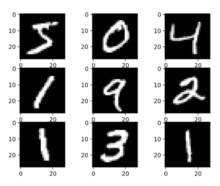
The first dataset employed here is the usual MNIST pixel data, comprised by hand-written numbers. Here, the background is black and the digits are white.
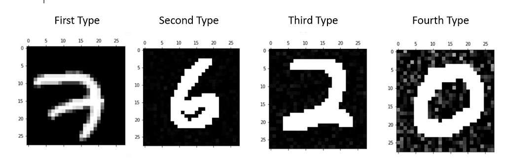
To test the new procedure and compare it to the usual one, I created four simple types of anomalous data.
The goal was to test each method’s detection capabilities across a small spectrum of noise variations, incrementally intensified from one anomaly type to the next.
The noise rate increases from the first to the fourth type of anomalous data. As you can see in the figure below, in the first and second types of data, the noise is not even detectable to the naked eye, while in the third type, you can already spot some white pixels.
Model-state data
While MNIST pixel data, with its hand-written digits against a stark backdrop, provides a classic foundation for anomaly detection, we’re trying something else. It’s a bit of a leap, taking us right into the core of the trained ANN to see what the neurons are up to. This could give us a whole new angle on spotting anomalies.
As mentioned, this model state data is comprised by the state of the neurons in an ANN when trained with MNIST data. As such, to generate this data, we start with training a simple ANN with MNIST pixel data, both with normal and anomalous data (the anomalous are comprised by the noisy data showed before in Figure 2).
We then perform the usual: split the data into training and testing, and then we fit the ANN model:
model.fit(X_train,Y_cat_train,epochs=8, validation_data=(X_test, y_cat_test))
After that, we want to retrieve the names of the layers in model and store them in a list:
list(map(lambda x: x.name, model.layers))
Finally, we create a new model that takes the same input as the original model but produces output from a specific layer called “dense”:
intermediate_layer_model=Model(inputs=model.input, outputs=model.get_layer("dense").output)
This is useful for extracting information from intermediate layers of a neural network.
Let’s take a look at this model-state data:
model_state_data_layer1=pd.read_csv("first_layer_dense.csv",header=None)
model_state_data_layer2=pd.read_csv("second_layer_dense.csv",header=None)

model_state_data_layer1.head(4)

The model-state data of the first neural layer is comprised by 32 columns and 4 rows.
With just a few lines of code, we are able to extract data from the intermediate layers of a neural network.
To study the effectiveness of the new method, I’ll be using data from both the first and second layers of the neural network.
As mentioned, the goal is to compare the anomaly detection task using two different input datasets across two different models: an ANN classifier and an Isolation Forest model. This comparison seeks to understand how each model performs with different types of input data in identifying anomalies.
The ANN:
An Artificial Neural Network (ANN) is a model inspired by the human brain’s network of neurons, designed to recognize patterns and process data in a manner similar to the way a human brain operates.
from tensorflow.keras.models import Sequential
from tensorflow.keras.layers import Dense, Dropout
from tensorflow.keras.optimizers import SGD
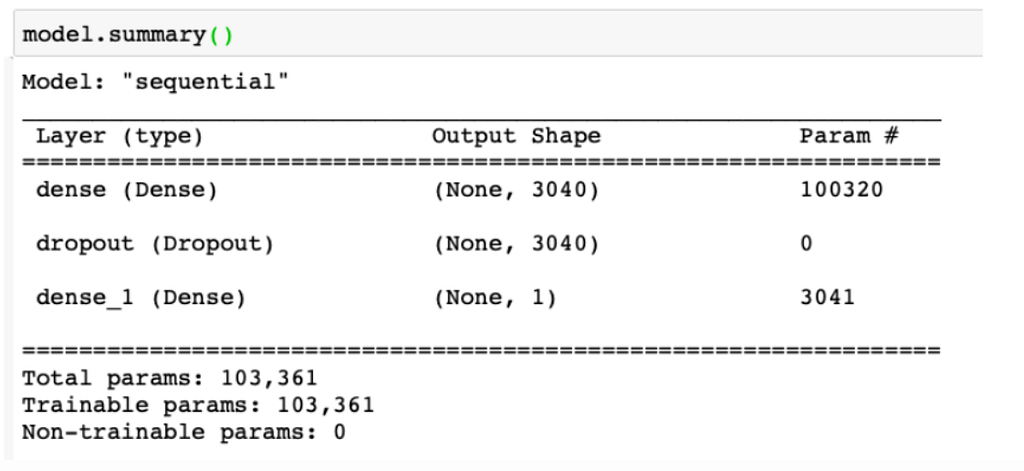
model = Sequential()
model.add(Dense(X_train.shape[1], input_shape=(784,), activation='relu'))
model.add(Dropout(0.2))
model.add(Dense(1, activation='sigmoid'))
model.compile(loss="binary_crossentropy", optimizer='adam', metrics=["accuracy"])
The Isolation Forest:
from sklearn.ensemble import IsolationForest
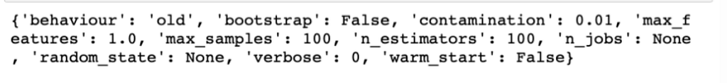
model = IsolationForest(max_samples=100, contamination=0.01)
model.fit(X_train)
Isolation forest is an unsupervised machine learning model for data anomaly detection. It employs binary trees to detect anomalies and, contrary to a Random Forest model, the selection of the splitting points of each branch is done randomly. This random splitting is efficient to isolate anomalies from normal observations. Since anomalies are few and different, they’re easier to separate with fewer random splits compared to normal data.
The second code line creates an instance of the IsolationForest class, setting max_samples to 100 which determines the number of samples to draw from X to train each base estimator, and contamination to 0.01 which is the expected proportion of outliers in the data.
print(model.get_params())
In this project, the aim was to assess the efficacy of anomaly detection by utilizing two distinct datasets across two models: a straightforward Artificial Neural Network (ANN) and the Isolation Forest model. This comparison seeks to understand how each model performs with different types of input data in identifying anomalies.
Inspecting True Positives
Both datasets are fed into an ANN.
First, let’s inspect the percentage of anomalies that both methods were able to detect:

Figure 6 shows the results when feeding an ANN with pixel data. The y-axis represents the anomaly score, in which data points with a threshold > 0.45 are considered anomalies. The different anomaly types are depicted in the plot with different colors.

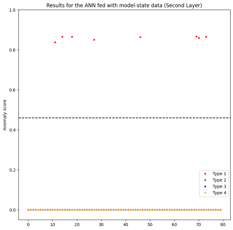
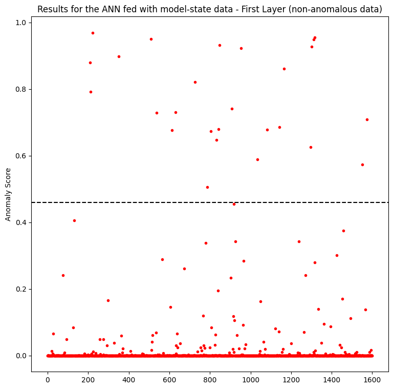
Figure 7 showcases the detection capabilities of the model-state method across two different neural layers, providing insights into how each layer’s data influences anomaly detection results.
Inspecting the left plot concerning the first layer, we can see that the new method detects more true positives (anomalies) regarding type 3 than the usual approach with the pixel data (Figure 6). The second layer is not useful at all, only predicting some anomalies of type 1.
However, it predicts anomalies of type 3 with low confidence, when compared to the pixel data method. Besides, the first layer does not predict well the anomalies of type 1,2 and 4. Interestingly, anomalies of types 1 and 4 represent the least and most noisy data, respectively.
Also curious to note is the statistical distribution of the data in the plots. In the normal data approach, the predictions are more scattered, and in the model-state one it is almost the opposite scenario.
Inspecting False Positives

In anomaly detection tasks, achieving a balance between precision and recall is crucial. Recall, in the context of anomaly detection, represents the ability of the model to correctly identify all actual anomalies in the dataset.
However, it’s often important to prioritize precision over recall in these tasks. This is because false positives (instances where normal data is wrongly classified as anomalous) can have significant consequences, such as triggering unnecessary alarms or interventions. In situations where it is risky to have a high rate of false positives, maintaining a low recall helps minimize the number of false alarms.
It is clear from the plots that the model-state approach performs much better on detecting true negatives, with the obvious benefit of discerning false positives. In this case, the first layer outperforms the second one:
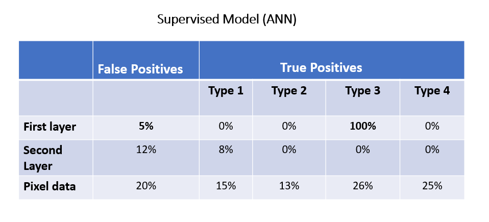
The model-state data of the first layer outperforms the second layer and pixel data in detecting types 2 and 3 anomalies and in identifying false positives. However, normal data still exhibits better performance in detecting types 1 and 4 anomalies.
2. Isolation Forest Results
Inspecting True Positives
Isolation forest computes a negative anomaly score, in which the smaller (more negative) the score, the more anomalous the data point is considered to be. We considered a threshold of < -0.45 to be considered anomalous.
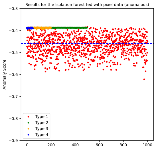
The isolation forest model when fed with pixel data, predicted 54% of the anomalous data of type 1 and predicted no anomalies of the other types.
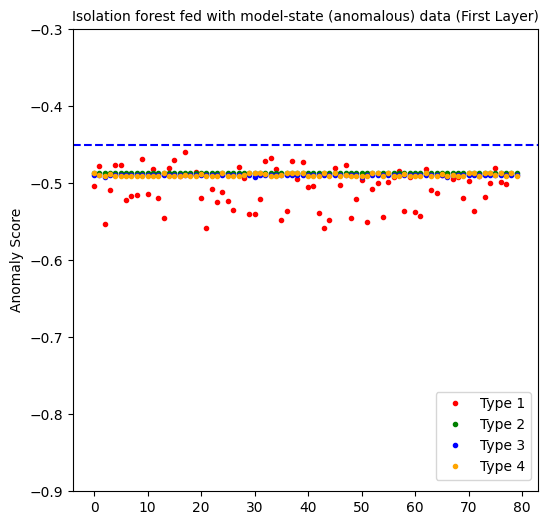

The first layer perfectly predicts all the anomalous data points. But as you will sew below, it also generates a 100% false positive rate. At the end, it is not an effective approach.
The second layer yields interesting results. With 100% of true positives for the second, third and fourth type of noisy types, it sounds promising on detecting certain kinds of anomalous data. The only downside is predicting 19% of anomalous data points for the 1st type of noisy data. But not that these are the hardest anomalies to detect, given that the noise ratio is the lowest!
Inspecting False Positives
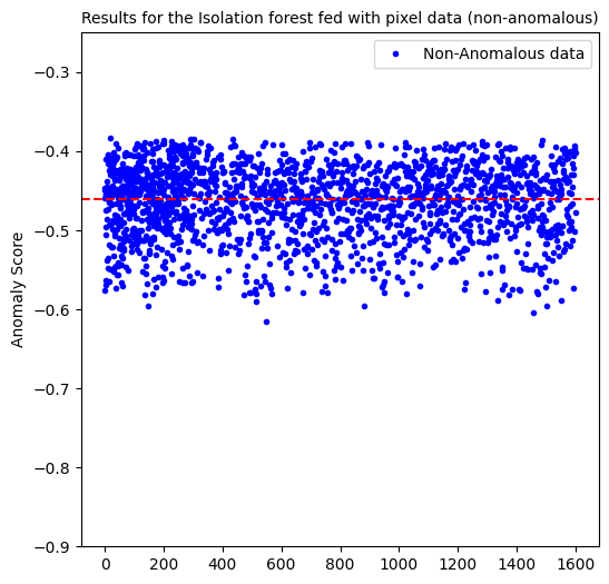
Here, the percentage of false positives is 50%. As good as flipping a coin!
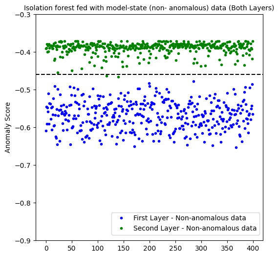
Inspecting how model-state data from different layers behave in predicting non-anomalous data, we see that the first layer predicted 100% of false positives whereas the second layer only 1%.

When fed with the usual pixel data, we are only able to predict 54% of anomalies of type 1 and besides, we are left with a false positive percentage of 50%.
On the other hand, the procedure employing model-state yields curious results especially regarding the second layer.
In conclusion, the results obtained from comparing the anomaly detection performance of an ANN and an Isolation Forest model using two different input data types provide valuable insights.
Even though this project was a preliminary experiment, I believe it underscores the importance of trying new strategies in detecting anomalies.
A potential possibility for future exploration could be combining both methods within the ANN framework — utilizing normal data to capture certain anomalies and model-state data to detect others.
This project not only contributed to the understanding of anomaly detection methodologies but also underscored the importance of exploring innovative approaches, such as utilizing the state of neurons, to enhance the performance of anomaly detection models!
Another thing this project taught me. As mentioned, it was my very first experience at a real company and I was scared of messing up. Either if you are a beginner or an experienced data scientist, if you’re feeling unsure about taking on a project because it seems daunting or you doubt your skills, remember that success in these projects isn’t just about what you already know; it’s about your willingness to learn and push through the fear. So, go for it!
What are your thoughts on utilizing neuron states for anomaly detection?
Thanks a million for reading.
My name is Sara Nóbrega and I am an R&D Engineer focused on Data Science, with a background in physics and astrophysics. I’m an enthusiast on AI, smart cities, sustainability, cosmology and human rights.
An Exploration of Model-State Data in Anomaly Detection was originally published in Towards Data Science on Medium, where people are continuing the conversation by highlighting and responding to this story.
Originally appeared here:
An Exploration of Model-State Data in Anomaly Detection
Go Here to Read this Fast! An Exploration of Model-State Data in Anomaly Detection

Neural networks are indeed powerful. However, as the application scope of neural networks moves from “standard” classification and regression tasks to more complex decision-making and AI for Science, one drawback is becoming increasingly apparent: the output of neural networks is usually unconstrained, or more precisely, constrained only by simple 0–1 bounds (Sigmoid activation function), non-negative constraints (ReLU activation function), or constraints that sum to one (Softmax activation function). These “standard” activation layers have been used to handle classification and regression problems and have witnessed the vigorous development of deep learning. However, as neural networks started to be widely used for decision-making, optimization solving, and other complex scientific problems, these “standard” activation layers are clearly no longer sufficient. This article will briefly discuss the current methodologies available that can add constraints to the output of neural networks, with some personal insights included. Feel free to critique and discuss any related topics.
If you are familiar with reinforcement learning, you may already know what I am talking about. Applying constraints to an n-dimensional vector seems difficult, but you can break an n-dimensional vector into n outputs. Each time an output is generated, you can manually write the code to restrict the action space for the next variable to ensure its value stays within a feasible domain. This so-called “autoregressive” method has obvious advantages: it is simple and can handle a rich variety of constraints (as long as you can write the code). However, its disadvantages are also clear: an n-dimensional vector requires n calls to the network’s forward computation, which is inefficient; moreover, this method usually needs to be modeled as a Markov Decision Process (MDP) and trained through reinforcement learning, so common challenges in reinforcement learning such as large action spaces, sparse reward functions, and long training times are also unavoidable.
In the domain of solving combinatorial optimization problems with neural networks, the autoregressive method coupled with reinforcement learning was once mainstream, but it is currently being replaced by more efficient methods.
During training, a penalty term can be added to the objective function, representing the degree to which the current neural network output violates constraints. In the traditional optimization field, the Lagrangian dual method also offers a similar trick. Unfortunately, when applied to neural networks, these methods have so far only been proven on some simple constraints, and it is still unclear whether they are applicable to more complex constraints. One shortcoming is that inevitably some of the model’s capacity is used to learn how to meet corresponding constraints, thereby limiting the model’s ability in other directions (such as optimization solving).
For example, Karalias and Loukas, NeurIPS’21 “Erdo˝s Goes Neural: an Unsupervised Learning Framework for Combinatorial Optimization on Graphs” demonstrated that the so-called “box constraints”, where variable values lie between [a, b], can be learned through a penalty term, and the network can solve some relatively simple combinatorial optimization problems. However, our further study found that this methodology lacks generalization ability. In the training set, the neural network can maintain constraints well; but in the testing set, the constraints are almost completely lost. Moreover, although adding a penalty term in principle can apply to any constraint, it cannot handle more difficult constraints. Our paper Wang et al, ICLR’23 “Towards One-Shot Neural Combinatorial Optimization Solvers: Theoretical and Empirical Notes on the Cardinality-Constrained Case” discusses the above phenomena and presents the theoretical analysis.
On the other hand, the design philosophy of generative models, where outputs need to conform to a specific distribution, seems more suited to the “learning constraints” approach. Sun and Yang, NeurIPS’23 “DIFUSCO: Graph-based Diffusion Solvers for Combinatorial Optimization” showed that Diffusion models can output solutions that meet the constraints of the Traveling Salesman Problem (i.e., can output a complete circuit). We further presented Li et al, NeurIPS’23 “T2T: From Distribution Learning in Training to Gradient Search in Testing for Combinatorial Optimization”, where the generative model (Diffusion) is responsible for meeting constraints, with another optimizer providing optimization guidance during the gradual denoising process of Diffusion. This strategy performed pretty well in experiments, surpassing all previous neural network solvers.
Maybe you are concerned that autoregressive is too inefficient, and generative models may not solve your problem. You might be thinking about a neural network that does only one forward pass, and the output needs to meet the given constraints — is that possible?
The answer is yes. We can solve a convex optimization problem to project the neural network’s output into a feasible domain bounded by convex constraints. This methodology utilizes the property that a convex optimization problem is differentiable at its KKT conditions so that this projection step can be regarded as an activation layer, embeddable in an end-to-end neural network. This methodology was proposed and promoted by Zico Kolter’s group at CMU, and they currently offer the cvxpylayers package to ease the implementation steps. The corresponding convex optimization problem is
where y is the unconstrained neural network output, x is the constrained neural network output. Because the purpose of this step is just a projection, a linear objective function can achieve this (adding an entropy regularizer is also reasonable). Ax ≤ b are the linear constraints you need to apply, which can also be quadratic or other convex constraints.
It is a personal note: there seem to be some known issues, and it seems that this repository has not been updated/maintained for a long time (04/2024). I would truly appreciate it if anyone is willing to investigate what is going on.
Deriving gradients using KKT conditions is theoretically sound, but it cannot tackle non-convex or non-continuous problems. In fact, for non-continuous problems, when changes in problem parameters cause solution jumps, the real gradient becomes a delta function (i.e., infinite at the jump), which obviously can’t be used in training neural networks. Fortunately, there are some gradient approximation methods that can tackle this problem.
The Georg Martius group at Max Planck Institute introduced a black-box approximation method Vlastelica et al, ICLR’2020 “Differentiation of Blackbox Combinatorial Solvers”, which views the solver as a black box. It first calls the solver once, then perturbs the problem parameters in a specific direction, and then calls the solver again. The residual between the outputs of the two solver calls serves as the approximate gradient. If this methodology is applied to the output of neural networks to enforce constraints, we can define an optimization problem with a linear objective function:
where y is the unconstrained neural network output, and x is the constrained neural network output. Your next step is to implement an algorithm to solve the above problem (not necessarily to be optimal), and then it can be integrated into the black-box approximation framework. A drawback of the black-box approximation method is that it can only handle linear objective functions, but a linear objective function just happens to work if you are looking for some methods to enforce constraints; moreover, since it is just a gradient approximation method if the hyperparameters are not well-tuned, it might encounter sparse gradients and convergence issues.
Another method for approximating gradients involves using a large amount of random noise perturbation, repeatedly calling the solver to estimate a gradient, as discussed in Berthet et al, NeurIPS’2020 “Learning with Differentiable Perturbed Optimizers”. Theoretically, the gradient obtained this way should be similar to the gradient obtained through the LinSAT method (which will be discussed in the next section), being the gradient of an entropy-regularized linear objective function; however, in practice, this method requires a large number of random samples, which is kind of impractical (at least on my use cases).
Whether it’s deriving gradients from KKT conditions for convex problems or approximating gradients for non-convex methods, both require calling/writing a solver, whereby the CPU-GPU communication could be a bottleneck because most solvers are usually designed and implemented for CPUs. Is there a way to project specific constraints directly on the GPU like an activation layer, without solving optimization problems explicitly?
The answer is yes, and our Wang et al, ICML’2023 “LinSATNet: The Positive Linear Satisfiability Neural Networks” presents a viable path and derives the convergence property of the algorithm. LinSAT stands for Linear SATisfiability Network.
LinSAT can be seen as an activation layer, allowing you to apply general positive linear constraints to the output of a neural network.
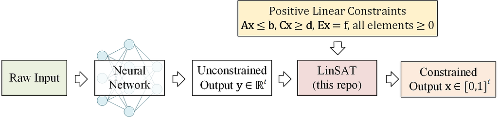
The LinSAT layer is fully differentiable, and the real gradients are computed by autograd, just like other activation layers. Our implementation now supports PyTorch.
You can install it by
pip install linsatnet
And get started with
from LinSATNet import linsat_layer
If you download and run the source code, you will find a simple example. In this example, we apply doubly stochastic constraints to a 3×3 matrix.
To run the example, first clone the repo:
git clone https://github.com/Thinklab-SJTU/LinSATNet.git
Go into the repo, and run the example code:
cd LinSATNet
python LinSATNet/linsat.py
In this example, we try to enforce doubly-stochastic constraints to a 3×3 matrix. The doubly stochastic constraint means that all rows and columns of the matrix should sum to 1.
The 3×3 matrix is flattened into a vector, and the following positive linear constraints are considered (for Ex=f):
E = torch.tensor(
    [[1, 1, 1, 0, 0, 0, 0, 0, 0],
     [0, 0, 0, 1, 1, 1, 0, 0, 0],
     [0, 0, 0, 0, 0, 0, 1, 1, 1],
     [1, 0, 0, 1, 0, 0, 1, 0, 0],
     [0, 1, 0, 0, 1, 0, 0, 1, 0],
     [0, 0, 1, 0, 0, 1, 0, 0, 1]], dtype=torch.float32
)
f = torch.tensor([1, 1, 1, 1, 1, 1], dtype=torch.float32)
We randomly init w and regard it as the output of some neural networks:
w = torch.rand(9) # w could be the output of neural network
w = w.requires_grad_(True)
We also have a “ground-truth target” for the output of linsat_layer, which is a diagonal matrix in this example:
x_gt = torch.tensor(
    [1, 0, 0,
     0, 1, 0,
     0, 0, 1], dtype=torch.float32
)
The forward/backward passes of LinSAT follow the standard PyTorch style and are readily integrated into existing deep learning pipelines.
The forward pass:
linsat_outp = linsat_layer(w, E=E, f=f, tau=0.1, max_iter=10, dummy_val=0)
The backward pass:
loss = ((linsat_outp — x_gt) ** 2).sum()
loss.backward()
You can also set E as a sparse matrix to improve the time & memory efficiency (especially for large-sized input). Here is a dumb example (consider to construct E in sparse for the best efficiency):
linsat_outp = linsat_layer(w, E=E.to_sparse(), f=f, tau=0.1, max_iter=10, dummy_val=0)
We can also do gradient-based optimization over w to make the output of linsat_layer closer to x_gt. This is what happens when you train a
neural network.
niters = 10
opt = torch.optim.SGD([w], lr=0.1, momentum=0.9)
for i in range(niters):
 x = linsat_layer(w, E=E, f=f, tau=0.1, max_iter=10, dummy_val=0)
 cv = torch.matmul(E, x.t()).t() — f.unsqueeze(0)
 loss = ((x — x_gt) ** 2).sum()
 loss.backward()
 opt.step()
 opt.zero_grad()
 print(f’{i}/{niters}n’
 f’ underlying obj={torch.sum(w * x)},n’
 f’ loss={loss},n’
 f’ sum(constraint violation)={torch.sum(cv[cv > 0])},n’
 f’ x={x},n’
 f’ constraint violation={cv}’)
And you are likely to see the loss decreasing during the training steps.
For full API references, please check out the GitHub repository.
Warning, tons of math ahead! You can safely skip this part if you are just using LinSAT.
If you want to learn more details and proofs, please refer to the main paper.
Here we introduce the mechanism inside LinSAT. It works by extending the Sinkhorn algorithm to multiple sets of marginals (to our best knowledge, we are the first to study Sinkhorn with multi-sets of marginals). The positive linear constraints are then enforced by transforming the constraints into marginals.
Let’s start with the classic Sinkhorn algorithm. Given non-negative score matrix S with size m×n, and a set of marginal distributions on rows (non-negative vector v with size m) and columns (non-negative vector u with size n), where
the Sinkhorn algorithm outputs a normalized matrix Γ with size m×n and values in [0,1] so that
Conceptually, Γᵢ ⱼ means the proportion of uⱼ moved to vᵢ.
The algorithm steps are:
Note that the above formulation is modified from the conventional Sinkhorn formulation. Γᵢ ⱼ uⱼ is equivalent to the elements in the “transport” matrix in papers such as (Cuturi 2013). We prefer this new formulation as it generalizes smoothly to Sinkhorn with multi-set marginals in the following.
To make a clearer comparison, the transportation matrix in (Cuturi 2013) is P with size m×n, and the constraints are
Pᵢ ⱼ means the exact mass moved from uⱼ to vᵢ.
The algorithm steps are:
We discover that the Sinkhorn algorithm can generalize to multiple sets of marginals. Recall that Γᵢ ⱼ ∈ [0,1] means the proportion of uⱼ moved to vᵢ. Interestingly, it yields the same formulation if we simply replace u, v with another set of marginal distributions, suggesting the potential of extending the Sinkhorn algorithm to multiple sets of marginal distributions. Denote that there are k sets of marginal distributions that are jointly enforced to fit more complicated real-world scenarios. The sets of marginal distributions are
and we have:
It assumes the existence of a normalized Z ∈ [0,1] with size m×n, s.t.
i.e., the multiple sets of marginal distributions have a non-empty feasible region (you may understand the meaning of “non-empty feasible region” after reading the next section about how to handle positive linear constraints). Multiple sets of marginal distributions could be jointly enforced by traversing the Sinkhorn iterations over k sets of marginal distributions. The algorithm steps are:
In our paper, we prove that the Sinkhorn algorithm for multi-set marginals shares the same convergence pattern with the classic Sinkhorn, and its underlying formulation is also similar to the classic Sinkhorn.
Then we show how to transform the positive linear constraints into marginals, which are handled by our proposed multi-set Sinkhorn.
Encoding neural network’s output
For an l-length vector denoted as y (which can be the output of a neural network, also it is the input to linsat_layer), the following matrix is built
where W is of size 2 × (l + 1), and β is the dummy variable, the default is β = 0. y is put at the upper-left region of W. The entropic regularizer is then enforced to control discreteness and handle potential negative inputs:
The score matrix S is taken as the input of Sinkhorn for multi-set marginals.
From linear constraints to marginals
1) Packing constraint Ax ≤ b. Assuming that there is only one constraint, we rewrite the constraint as
Following the “transportation” view of Sinkhorn, the output x moves at most b unit of mass from a₁, a₂, …, aₗ, and the dummy dimension allows the inequality by moving mass from the dummy dimension. It is also ensured that the sum of uₚ equals the sum of vₚ. The marginal distributions are defined as
2 ) Covering constraint Cx ≥ d. Assuming that there is only one constraint, we rewrite the constraint as
We introduce the multiplier
because we always have
(else the constraint is infeasible), and we cannot reach a feasible solution where all elements in x are 1s without this multiplier. Our formulation ensures that at least d unit of mass is moved from c₁, c₂, …, cₗ by x, thus representing the covering constraint of “greater than”. It is also ensured that the sum of u_c equals the sum of v_c. The marginal distributions are defined as
3) Equality constraint Ex = f. Representing the equality constraint is more straightforward. Assuming that there is only one constraint, we rewrite the constraint as
The output x moves e₁, e₂, …, eₗ to f, and we need no dummy element in uₑ because it is an equality constraint. It is also ensured that the sum of uₑ equals the sum of vₑ. The marginal distributions are defined as
After encoding all constraints and stacking them as multiple sets of marginals, we can call the Sinkhorn algorithm for multi-set marginals to encode the constraints.
In our ICML paper, we validated the LinSATNet method for routing constraints beyond the general case (used for solving variants of the Traveling Salesman Problem), partial graph matching constraints (used in graph matching where only subsets of graphs match each other), and general linear constraints (used in specific preference with portfolio optimization). All these problems can be represented with positive linear constraints and handled using the LinSATNet method. In experiments, neural networks are capable of learning how to solve all three problems.
It should be noted that the LinSATNet method can only handle positive linear constraints, meaning that it is unable to handle constraints like x₁ — x₂ ≤ 0 which contain negative terms. However, positive linear constraints already cover a vast array of scenarios. For each specific problem, the mathematical modeling is often not unique, and in many cases, a reasonable positive linear formulation could be found. In addition to the examples mentioned above, let the network output organic molecules (represented as graphs, ignoring hydrogen atoms, considering only the skeleton) can consider constraints such as C atoms having no more than 4 bonds, O atoms having no more than 2 bonds.
Adding constraints to neural networks has a wide range of application scenarios, and so far, several methods are available. It’s important to note that there is no golden standard to judge their superiority over each other — the best method is usually relevant to a certain scenario.
Of course, I recommend trying out LinSATNet! Anyway, it is as simple as an activation layer in your network.
If you found this article helpful, please feel free to cite:
@inproceedings{WangICML23,
  title={LinSATNet: The Positive Linear Satisfiability Neural Networks},
  author={Wang, Runzhong and Zhang, Yunhao and Guo, Ziao and Chen, Tianyi and Yang, Xiaokang and Yan, Junchi},
  booktitle={International Conference on Machine Learning (ICML)},
  year={2023}
}
All aforementioned content has been discussed in this paper.
How to Encode Constraints to the Output of Neural Networks was originally published in Towards Data Science on Medium, where people are continuing the conversation by highlighting and responding to this story.
Originally appeared here:
How to Encode Constraints to the Output of Neural Networks
Go Here to Read this Fast! How to Encode Constraints to the Output of Neural Networks


Applying the 6 steps of the INSPIRe framework to accelerate your code generation (ChatGPT-4 — Claude 3 — Gemini)
Originally appeared here:
Advanced Code Generation With LLMs — Building a Synthetic Data Generator
Go Here to Read this Fast! Advanced Code Generation With LLMs — Building a Synthetic Data Generator


Use the INSPIRe framework to save time and gain a competitive edge (ChatGPT-4 — Claude 3 — Gemini)
Originally appeared here:
6 Steps to Make AI Write Your Python Code for You
Go Here to Read this Fast! 6 Steps to Make AI Write Your Python Code for You

Generalist Anomaly Detection (GAD) aims to train one single detection model that can generalize to detect anomalies in diverse datasets from different application domains without any further training on the target data.
Work to be published at CVPR 2024 [1].
Some recent studies have showed that large pre-trained Visual-Language Models (VLMs) like CLIP have strong generalization capabilities on detecting industrial defects from various datasets, but their methods rely heavily on handcrafted text prompts about defects, making them difficult to generalize to anomalies in other applications, e.g., medical image anomalies or semantic anomalies in natural images.
In this work, we propose to train a GAD model with few-shot normal images as sample prompts for AD on diverse datasets on the fly. To this end, we introduce a novel approach that learns an in–context residual learning model for GAD, termed InCTRL.
It is trained on an auxiliary dataset to discriminate anomalies from normal samples based on a holistic evaluation of the residuals between query images and few-shot normal sample prompts. Regardless of the datasets, per definition of anomaly, larger residuals are expected for anomalies than normal samples, thereby enabling InCTRL to generalize across different domains without further training.
Comprehensive experiments on nine AD datasets are performed to establish a GAD benchmark that encapsulate the detection of industrial defect anomalies, medical anomalies, and semantic anomalies in both one-vs-all and multi-class setting, on which InCTRL is the best performer and significantly outperforms state-of-the-art competing methods. Code is available at https://github.com/mala-lab/InCTRL.
Anomaly Detection (AD) is a crucial computer vision task that aims to detect samples that substantially deviate from the majority of samples in a dataset, due to its broad real-life applications such as industrial inspection, medical imaging analysis, and scientific discovery, etc. [2–3]. Current AD paradigms are focused on individually building one model on the training data, e.g.,, a set of anomaly-free samples, of each target dataset, such as data reconstruction approach, one-class classification, and knowledge distillation approach. Although these approaches have shown remarkable detection performance on various AD benchmarks, they require the availability of large training data and the skilled detection model training per dataset. Thus, they become infeasible in application scenarios where training on the target dataset is not allowed due to either data privacy issues, e.g., arising from using those data in training the models due to machine unlearning [3], or unavailability of large-scale training data in the deployment of new applications. To tackle these challenges, this work explores the problem of learning Generalist Anomaly Detection (GAD) models, aiming to train one single detection model that can generalize to detect anomalies in diverse datasets from different application domains without any training on the target data.
Being pre-trained on web-scale image-text data, large Visual-Language Models (VLMs) like CLIP have exhibited superior generalization capabilities in recent years, achieving accurate visual recognition across different datasets without any fine-tuning or adaptation on the target data. More importantly, some very recent studies (e.g., WinCLIP [5]) show that these VLMs can also be utilized to achieve remarkable generalization on different defect detection datasets. Nevertheless, a significant limitation of these models is their dependency on a large set of manually crafted prompts specific to defects. This reliance restricts their applicability, making it challenging to extend their use to detecting anomalies in other data domains, e.g., medical image anomalies or semantic anomalies in one-vs-all or multi-class settings.
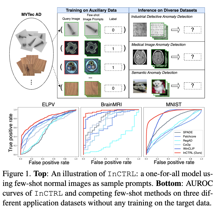
To address this problem, we propose to train a GAD model that aims to utilize few-shot normal images from any target dataset as sample prompts for supporting GAD on the fly, as illustrated in Figure 1(Top). The few-shot setting is motivated by the fact that it is often easy to obtain few-shot normal images in real-world applications. Furthermore, these few-shot samples are not used for model training/tuning; they are just used as sample prompts for enabling the anomaly scoring of test images during inference. This formulation is fundamentally different from current few-shot AD methods that use these target samples and their extensive augmented versions to train the detection model, which can lead to an overfitting of the target dataset and fail to generalize to other datasets, as shown in Figure 1(Bottom).
We then introduce an GAD approach, the first of its kind, that learns an in–context residual learning model based on CLIP, termed InCTRL. It trains an GAD model to discriminate anomalies from normal samples by learning to identify the residuals/discrepancies between query images and a set of few-shot normal images from auxiliary data. The few-shot normal images, namely in-context sample prompts, serve as prototypes of normal patterns. When comparing with the features of these normal patterns, per definition of anomaly, a larger residual is typically expected for anomalies than normal samples in datasets of different domains, so the learned in-context residual model can generalize to detect diverse types of anomalies across the domains. To capture the residuals better, InCTRL models the in-context residuals at both the image and patch levels, gaining an in-depth in-context understanding of what constitutes an anomaly. Further, our in-context residual learning can also enable a seamless incorporation of normal/abnormal text prompt-guided prior knowledge into the detection model, providing an additional strength for the detection from the text-image-aligned semantic space.
Extensive experiments on nine AD datasets are performed to establish a GAD benchmark that encapsulates three types of popular AD tasks, including industrial defect anomaly detection, medical image anomaly detection, and semantic anomaly detection under both one-vs-all and multi-class settings. Our results show that InCTRL significantly surpasses existing state-of-the-art methods.
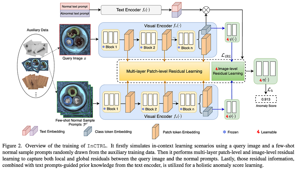
Our approach InCTRL is designed to effectively model the in-context residual between a query image and a set of few-shot normal images as sample prompts, utilizing the generalization capabilities of CLIP to detect unusual residuals for anomalies from different application domains.
CLIP is a VLM consisting of a text encoder and a visual encoder, with the image and text representations from these encoders well aligned by pre-training on web-scale text-image data. InCTRL is optimized using auxiliary data via an in-context residual learning in the image encoder, with the learning augmented by text prompt-guided prior knowledge from the text encoder.
To be more specific, as illustrated in Fig.2, we first simulate an in-context learning example that contains one query image x and a set of few-shot normal sample prompts P’, both of which are randomly sampled from the auxiliary data. Through the visual encoder, we then perform multi-layer patch-level and image-level residual learning to respectively capture local and global discrepancies between the query and few-shot normal sample prompts. Further, our model allows a seamless incorporation of normal and abnormal text prompts-guided prior knowledge from the text encoder based on the similarity between these textual prompt embeddings and the query images . The training of InCTRL is to optimize a few projection/adaptation layers attached to the visual encoder to learn a larger anomaly score for anomaly samples than normal samples in the training data, with the original parameters in both encoders frozen; during inference, a test image, together with the few-shot normal image prompts from the target dataset and the text prompts, is put forward through our adapted CLIP-based GAD network, whose output is the anomaly score for the test image.
Datasets and Evaluation Metrics. To verify the efficiency of our method, we conduct comprehensive experiments across nine real-world AD datasets, including five industrial defect inspection dataset (MVTec AD, VisA, AITEX, ELPV, SDD), two medical image datasets (BrainMRI, HeadCT), and two semantic anomaly detection datasets: MNIST and CIFAR-10 under both one-vs-all and multi-class protocols. Under the one-vs-all protocol, one class is used as normal, with the other classes treated as abnormal; while under the multi-class protocol, images of even-number classes from MNIST and animal-related classes from CIFAR-10 are treated as normal, with the images of the other classes are considered as anomalies.
To assess the GAD performance, MVTec AD, the combination of its training and test sets, is used as the auxiliary training data, on which GAD models are trained, and they are subsequently evaluated on the test set of the other eight datasets without any further training. We train the model on VisA when evaluating the performance on MVTec AD.
The few-shot normal prompts for the target data are randomly sampled from the training set of target datasets and remain the same for all models for fair comparison. We evaluate the performance with the number of few-shot normal prompt set to K = 2, 4, 8. The reported results are averaged over three independent runs with different random seeds.
As for evaluation metrics, we use two popular metrics AUROC (Area Under the Receiver Operating Characteristic) and AUPRC (Area Under the Precision-Recall Curve) to evaluate the AD performance.
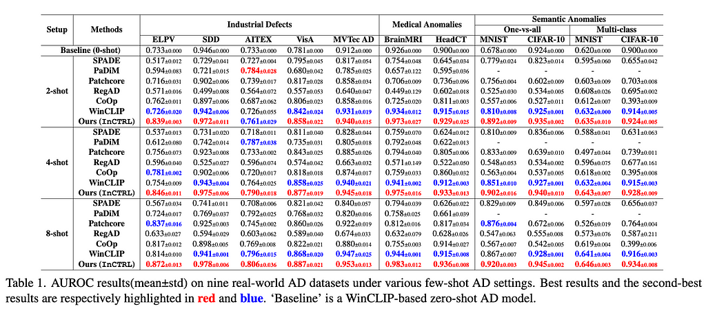
Results. The main results are reporeted in Tables 1 and 2. For the 11 industrial defect AD datasets, InCTRL significantly outperforms all competing models on almost all cases across the three few-shot settings in both AUROC and AUPRC. With more few-shot image prompts, the performance of all methods generally gets better. InCTRL can utilize the increasing few-shot samples well and remain the superiority over the competing methods.
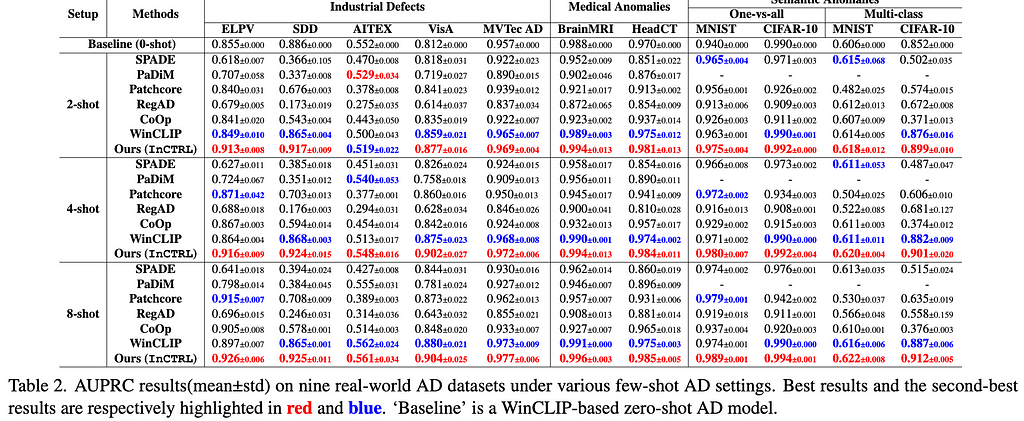
Ablation Study. We examine the contribution of three key components of our approach on the generalization: text prompt-guided features (T), patch-level residuals (P), and image-level residuals (I), as well as their combinations. The results are reported in Table 3. The experiment results indicate that for industrial defect AD datasets, visual residual features play a more significant role compared to text prompt-based features, particularly on datasets like ELPV, SDD, and AITEX. On the medical image AD datasets, both visual residuals and textual knowledge contribute substantially to performance enhancement, exhibiting a complementary relation. On semantic AD datasets, the results are dominantly influenced by patch-level residuals and/or text prompt-based features. Importantly, our three components are generally mutually complementary, resulting in the superior detection generalization across the datasets.
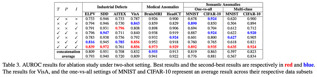
Significance of In-context Residual Learning. To assess the importance of learning the residuals in InCTRL, we experiment with two alternative operations in both multi-layer patch-level and image-level residual learning: replacing the residual operation with 1) a concatenation operation and 2) an average operation, with all the other components of InCTRL fixed. As shown in Table 3, the in-context residual learning generalizes much better than the other two alternative ways, significantly enhancing the model’s performance in GAD across three distinct domains.
In this work we introduce a GAD task to evaluate the generalization capability of AD methods in identifying anomalies across various scenarios without any training on the target datasets. This is the first study dedicated to a generalist approach to anomaly detection, encompassing industrial defects, medical anomalies, and semantic anomalies. Then we propose an approach, called InCTRL, to addressing this problem under a few-shot setting. InCTRL achieves a superior GAD generalization by holistic in-context residual learning. Extensive experiments are performed on nine AD datasets to establish a GAD evaluation benchmark for the aforementioned three popular AD tasks, on which InCTRL significantly and consistently outperforms SotA competing models across multiple few-shot settings.
Please check out the full paper [1] for more details of the approach and the experiments. Code is publicly available at https://github.com/mala-lab/InCTRL.
[1] Zhu, Jiawen, and Guansong Pang. “Toward Generalist Anomaly Detection via In-context Residual Learning with Few-shot Sample Prompts.” arXiv preprint arXiv:2403.06495 (2024).
[2] Pang, Guansong, et al. “Deep learning for anomaly detection: A review.” ACM computing surveys (CSUR) 54.2 (2021): 1–38.
[3] Cao, Yunkang, et al. “A Survey on Visual Anomaly Detection: Challenge, Approach, and Prospect.” arXiv preprint arXiv:2401.16402 (2024).
[4] Xu, Jie, et al. “Machine unlearning: Solutions and challenges.” IEEE Transactions on Emerging Topics in Computational Intelligence (2024).
[5] Jeong, Jongheon, et al. “Winclip: Zero-/few-shot anomaly classification and segmentation.” Proceedings of the IEEE/CVF Conference on Computer Vision and Pattern Recognition. 2023.
Learning Generalist Models for Anomaly Detection was originally published in Towards Data Science on Medium, where people are continuing the conversation by highlighting and responding to this story.
Originally appeared here:
Learning Generalist Models for Anomaly Detection
Go Here to Read this Fast! Learning Generalist Models for Anomaly Detection

In this post, I will be going over the implementation of a Self-evaluation RAG pipeline for question-answering using LangChain Expression Language (LCEL). The focus of this post will be on the use of LCEL for building pipelines and not so much on the actual RAG and self evaluation principles used, which are kept simple for ease of understanding.
I will be covering the following topics :
Before we jump into the development of the RAG chain, there are some basic setup steps that we need to perform to initialize this setup. These include :
The data ingestion consists of two key steps :
We will be using different prompts for the question-answering and self-evaluation tasks. We will be having 3 different prompt templates :
We initialize a simple vector database using FAISS and Open AI embeddings. For retrieval, we set k as 3 (return top 3 chunks for a given query)
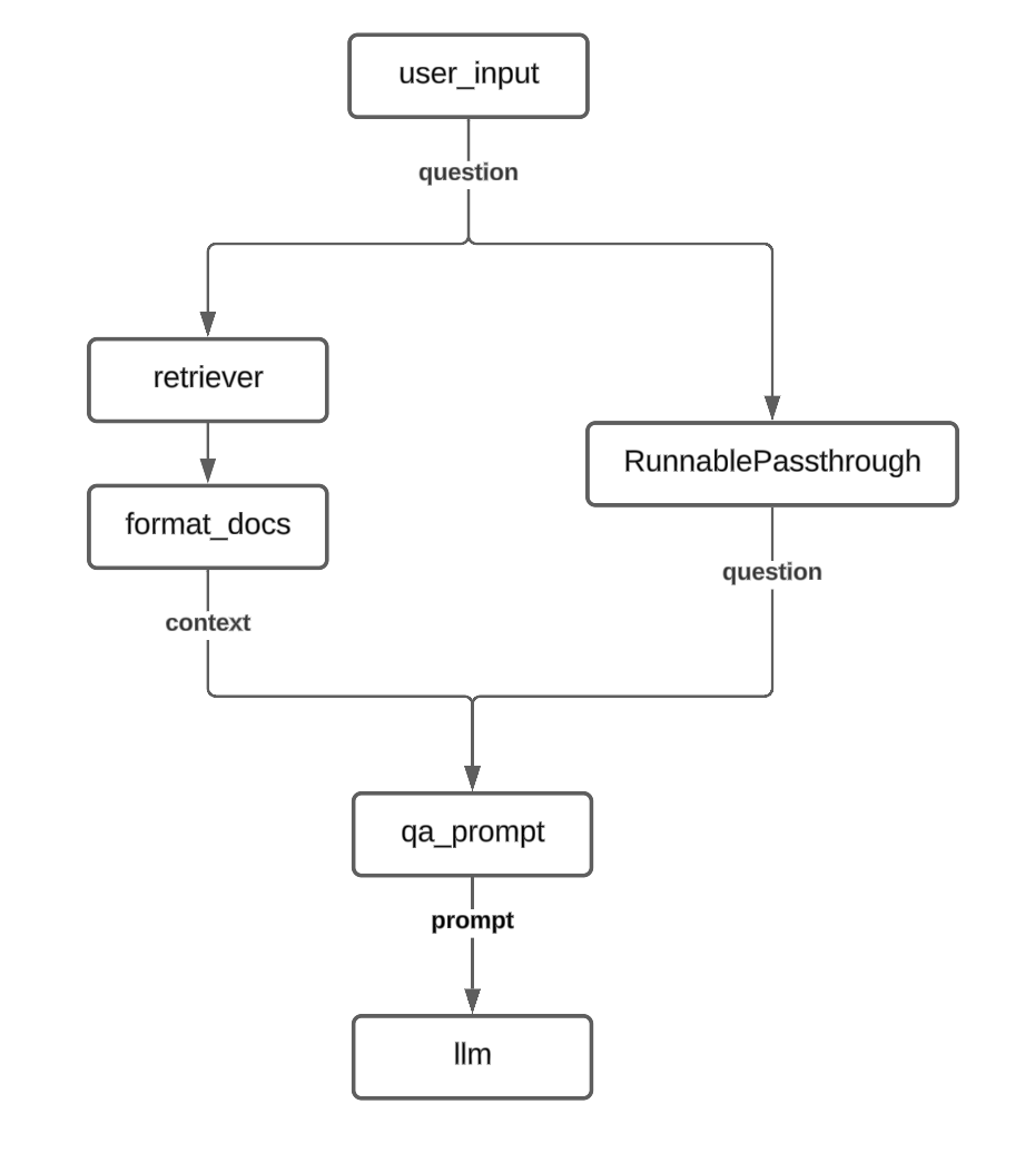
We start off with an example of a basic RAG chain that carries out the following steps :
Using LangChain Expression Language(LCEL), this RAG would be implemented as such:
rag_chain = (
            RunnableParallel(context = retriever | format_docs, question = RunnablePassthrough() ) |
            qa_prompt |
            llm
)
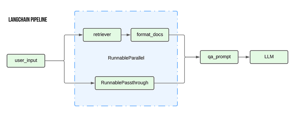
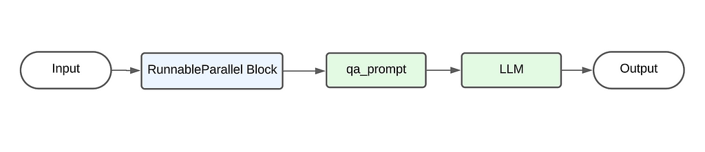
The above code primarily follows the pipe architecture where the output from the preceding element is used as the input for the next element. The below diagram showcases the flow of data. Starting from the user’s input, it passes first through the RunnableParallel block, then through the qa_prompt to generate the prompt. This prompt is then sent to the LLM to generate the final output.
There are two key additions to this pipeline that are unique to LangChain :
The flowchart for the above RAG would look like this :
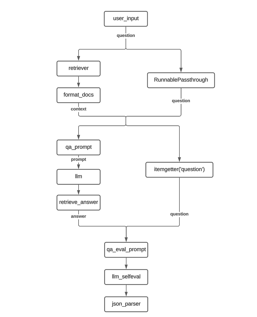
Building over the previous RAG chain, we now introduce new elements into the chain to implement the self evaluation component.
The self evaluation component is again a pretty straightforward implementation. We take the answer provided by the first LLM and pass it to the evaluator LLM along with the question and ask it to provide a binary response (Correct/Incorrect).
rag_chain = (
            RunnableParallel(context = retriever | format_docs, question = RunnablePassthrough() ) |
            RunnableParallel(answer= qa_prompt | llm | retrieve_answer, question = itemgetter("question") ) |
            qa_eval_prompt |
            llm_selfeval |
            json_parser
            )
The first key difference is the addition of an additional RunnableParallel component. This is required because, similar to the initial prompt for the QA, the self eval prompt also requires two inputs : the base LLM’s answer as well as the user’s question.
So the output of the first RunnableParallel is the context text and the question while the output of the second RunnableParallel is the LLM answer along with the question.
NOTE: For the second RunnableParallel, we use the itemgetter method to retain only the question value from the previous input and propagate it forward. This is done instead of using RunnablePassthrough as it would passed on the full input (dict with two keys) whereas we are only interested in passing on the question right now and not the context. Additionally, there is the issue of formatting as qa_eval_prompt expects a dict with str -> str mapping but using RunnablePassthrough would results in a str-> dict mapping
The flowchart for this RAG implementation would look like this:
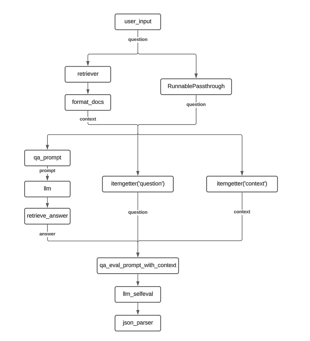
For this variation, we make a change to the evaluation procedure. In addition to the question-answer pair, we also pass the retrieved context to the evaluator LLM.
To accomplish this, we add an additional itemgetter function in the second RunnableParallel to collect the context string and pass it to the new qa_eval_prompt_with_context prompt template.
rag_chain = (
            RunnableParallel(context = retriever | format_docs, question = RunnablePassthrough() ) |
            RunnableParallel(answer= qa_prompt | llm | retrieve_answer, question = itemgetter("question"), context = itemgetter("context") ) |
            qa_eval_prompt_with_context |
            llm_selfeval |
            json_parser
            )
Implementation Flowchart :
One of the common pain points with using a chain implementation like LCEL is the difficulty in accessing the intermediate variables, which is important for debugging pipelines. We look at few options where we can still access any intermediate variables we are interested using manipulations of the LCEL
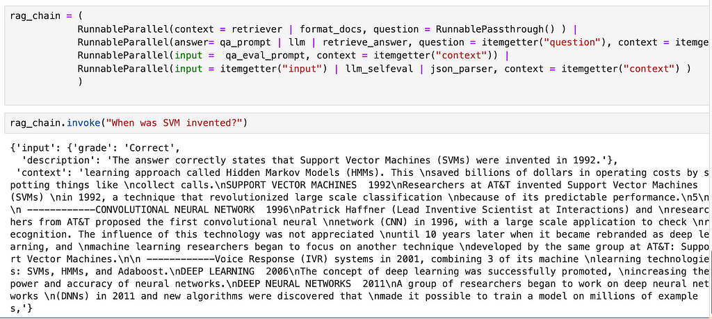
As we saw earlier, RunnableParallel allows us to carry multiple arguments forward to the next step in the chain. So we use this ability of RunnableParallel to carry forward the required intermediate values all the way till the end.
In the below example, we modify the original self eval RAG chain to output the retrieved context text along with the final self evaluation output. The primary change is that we add a RunnableParallel object to every step of the process to carry forward the context variable.
Additionally, we also use the itemgetter function to clearly specify the inputs for the subsequent steps. For example, for the last two RunnableParallel objects, we use itemgetter(‘input’) to ensure that only the input argument from the previous step is passed on to the LLM/ Json parser objects.
rag_chain = (
            RunnableParallel(context = retriever | format_docs, question = RunnablePassthrough() ) |
            RunnableParallel(answer= qa_prompt | llm | retrieve_answer, question = itemgetter("question"), context = itemgetter("context") ) |
            RunnableParallel(input =  qa_eval_prompt, context = itemgetter("context")) |
            RunnableParallel(input = itemgetter("input") | llm_selfeval , context = itemgetter("context") ) |
            RunnableParallel(input = itemgetter("input") | json_parser,  context = itemgetter("context") )
            )
The output from this chain looks like the following :
A more concise variation:
rag_chain = (
            RunnableParallel(context = retriever | format_docs, question = RunnablePassthrough() ) |
            RunnableParallel(answer= qa_prompt | llm | retrieve_answer, question = itemgetter("question"), context = itemgetter("context") ) |
            RunnableParallel(input =  qa_eval_prompt | llm_selfeval | json_parser, context = itemgetter("context"))
            )
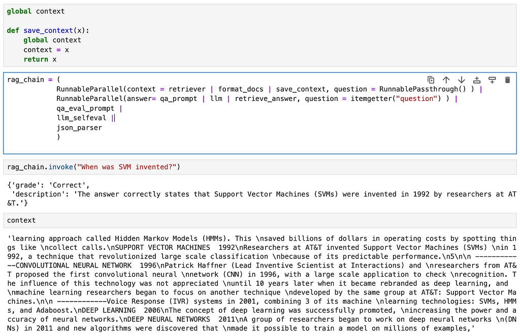
This method essentially uses the principle of a logger. We introduce a new function that saves its input to a global variable, thus allowing us access to the intermediate variable through the global variable
global context

def save_context(x):
    global context
    context = x
    return x

rag_chain = (
            RunnableParallel(context = retriever | format_docs | save_context, question = RunnablePassthrough() ) |
            RunnableParallel(answer= qa_prompt | llm | retrieve_answer, question = itemgetter("question") ) |
            qa_eval_prompt |
            llm_selfeval |
            json_parser
            )
Here we define a global variable called context and a function called save_context that saves its input value to the global context variable before returning the same input. In the chain, we add the save_context function as the last step of the context retrieval step.
This option allows you to access any intermediate steps without making major changes to the chain.
Attaching callbacks to your chain is another common method used for logging intermediate variable values. Theres a lot to cover on the topic of callbacks in LangChain, so I will be covering this in detail in a different post.
The reasons for using LCEL are best explained by the authors of Langchain themselves in their official documentation.
Of the points mentioned in the documentation, the following are some that I find especially useful :
Above these reasons, as a matter of personal preference, I feel that using LCEL helps improve the readability of your code and allows for cleaner implementations.
Images : All images are created by the author
In addition to Medium, I share my thoughts, ideas and other updates on Linkedin.
Building a RAG chain using LangChain Expression Language (LCEL) was originally published in Towards Data Science on Medium, where people are continuing the conversation by highlighting and responding to this story.
Originally appeared here:
Building a RAG chain using LangChain Expression Language (LCEL)
Go Here to Read this Fast! Building a RAG chain using LangChain Expression Language (LCEL)


Abstraction is one of the most critical concepts in Computer Science, with some of the most powerful implications. From a simplistic point of view, abstraction is the ability to take something and apply it to multiple distinct situations. For example, if you create a way to successfully sort apples based on their size in a factory, your solution could be abstracted to also sort oranges or peaches in the same way. Thus, through abstraction a very powerful solution is able to radically impact multiple parts of the world.
While Large Language Models are exceptional at reasoning when given text as an input, recently we have been able to abstract their input so that they can reason with images and sounds.
The below blog post goes into architectural ablations in Apple’s MM1 paper and their research findings when building a Multimodal Large Language Model (MLLM).
The architecture behind Large Language Models can be traced back to the 2017 paper “Attention is All You Need” where the Transformer Architecture was introduced.
This paper showed how you could transform human language into tokens that a neural network would then process (in that paper’s case, process into a different language).

As you can see from the image, we have a transformation occurring early on where we take the input and convert it into tokens (the embedding section). However, there is no inherent reason why only text data can be mapped to tokens. Consequently, the field began trying to map other kinds of data to tokens.

Apple’s model had 3 key components: a visual transformer (ViT) image encoder, Vision-Language Connector, and a Large Language Model. Assuming you already have a good idea of what a LLM is and how it works, let’s dive into the image encoder and VL connector.
While from an abstracted view we can imagine text and images as simply different kinds of inputs, to make this work we need to accept that we may have to treat them differently to get them into token form. At this time, we have 2 different systems that help us transform the image into tokens the LLM can reason with: image encoder and connector.
First, the image encoder is responsible for taking our image and converting it into the token representation that our transformer model can understand.
Second, a connector is the piece that takes data from the vision encoder and transforms it into the data that is passed directly to the large language model. Given the image encoder returns tokens, you may wonder why we need the connector at all. The idea appears to be that image encoders give too much information in their tokens, so to reduce costs while optimizing reasoning, we want to be selective with what we pass through.
The below image shows the data flow we’re working with here.
An ablation study in Machine Learning revolves around removing and modifying certain parts of a model to see how they contribute to overall performance. Apple’s research centered around different ways of training the Image Encoder, different projectors for the VL Connector, and different pre-training data.
Let’s dive into the major findings.
For the Image Encoder, they varied between CLIP and AIM models, Image resolution size, and the dataset the models were trained on. The below chart shows you the results for each ablation.
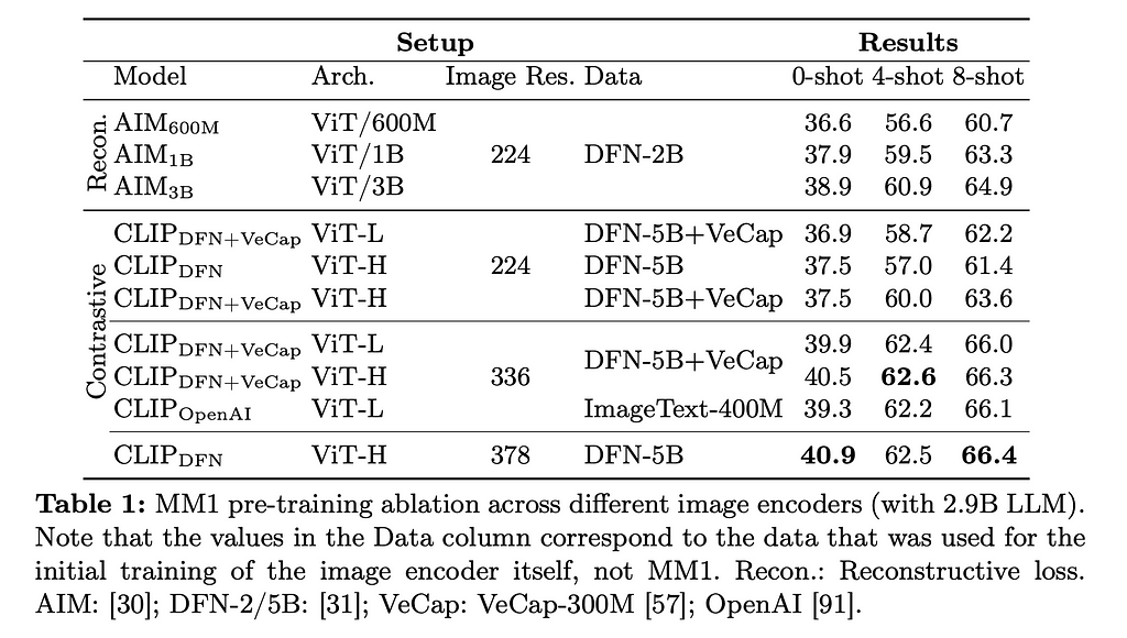
Let’s go through the major pieces above and explain what they are.
CLIP stands for Contrastive Language Image Pre-training and is meant to help your model learn visual concepts by providing names to the things that are meant to be seen as text. As the image below shows, this pairs images with text encodings so that the model will eventually connect the vision tokens (represented in the below image as I, with the text tokens T). This method is called contrastive training.
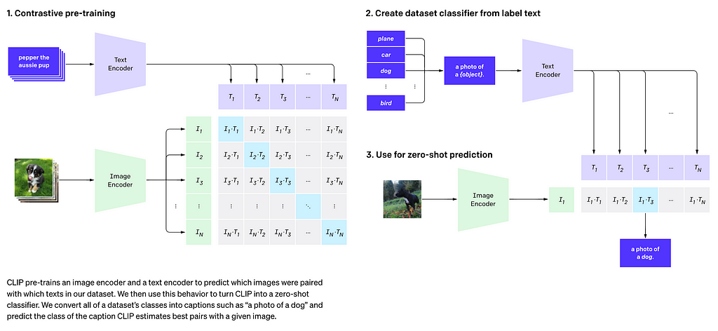
AIM stands for Autoregressive Image Model, and it is trained via a reconstructive loss optimization algorithm. The goal here is to see if the transformer can recreate (reconstruct) the image that it is given.

Image Resolution here refers to the number of pixels that is fed into the transformer. For example, a 378 x 378 image resolution means we will pass in a matrix of that size and then convert it into embeddings that the model will then be trained on. Training Data was split between the (DFN-2B), (DFN-5B), (DFN-5B + VeCap) and (ImageText-400M).
The authors found that image resolution was of highest importance, followed by model size and then the training data contents. Specifically, they saw that the better the image resolution, the better the model tended to perform for both zero-shot and few-shot prompting. As more compute is needed to train and run models with higher image resolution requirements, this suggests that for Vision Transformers, compute will remain of paramount importance.
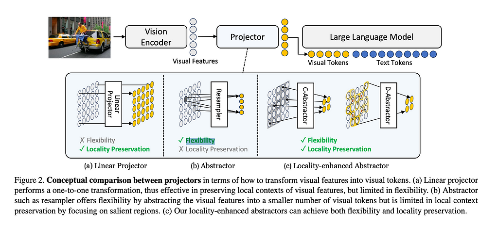
For the VL Connector, they tested using 64 or 144 tokens for the image, tested using 224, 336, and 378 for the image resolution, and chose between a few architectures. I’ll briefly go over the architectures below.
Average Pooling is exactly what it sounds like, taking the average of all of the tokens, and then doing a linear projection of this average so that the grid was 8×8 or 12×12.
Attention Pooling makes the assumption that image tokens should be treated as samples from a fundamentally different population set than the text tokens. Here we adjust how many tokens are fed in for each image, in the paper referred to as k learnable queries. The researchers only considered k of either 64 or 144.
Convolutional Mapping is a a method from Honeybee that uses a ResNet to dynamically decide how many tokens to pass through to the LLM from the image. This is actualized in the C-Abstractor module.

As you can see from the above, the different architectures actually had very little impact. As one might guess, the higher resolution images and the more tokens passed through increased performance among all of the connectors but not dramatically so.
This finding suggests we either haven’t found a significantly better way to connect the image encoder to the LLM, or that this area is simply not where great models will differentiate themselves.
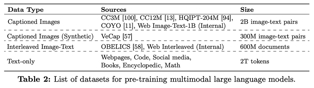
Here, the authors played with 4 different kinds of data: captioned images, synthetically captioned images, interleaved image-text data, and text-only data. They found 4 lessons, each with a graph to summarize the performance changes.
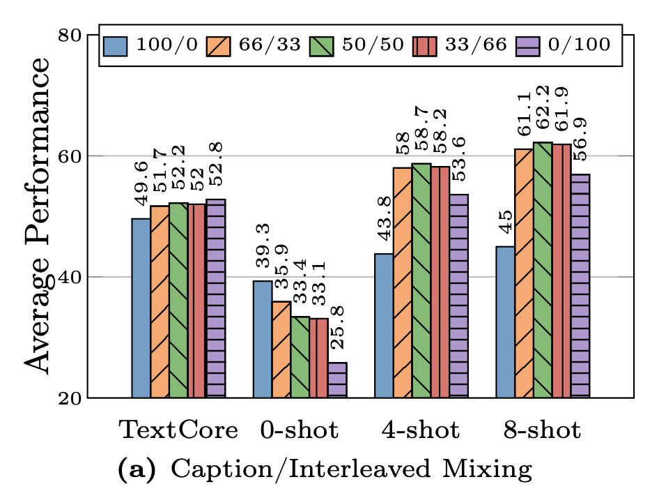
First, interleaving data helps with few-shot and text-only performance, while captioned data helps with zero-shot performance. The researchers varied how much interleaving they did, with the graph below showing the results. As you can see, few-shot prompts performed noticeably better on models trained with interleaved data than the models trained with all or nothing.
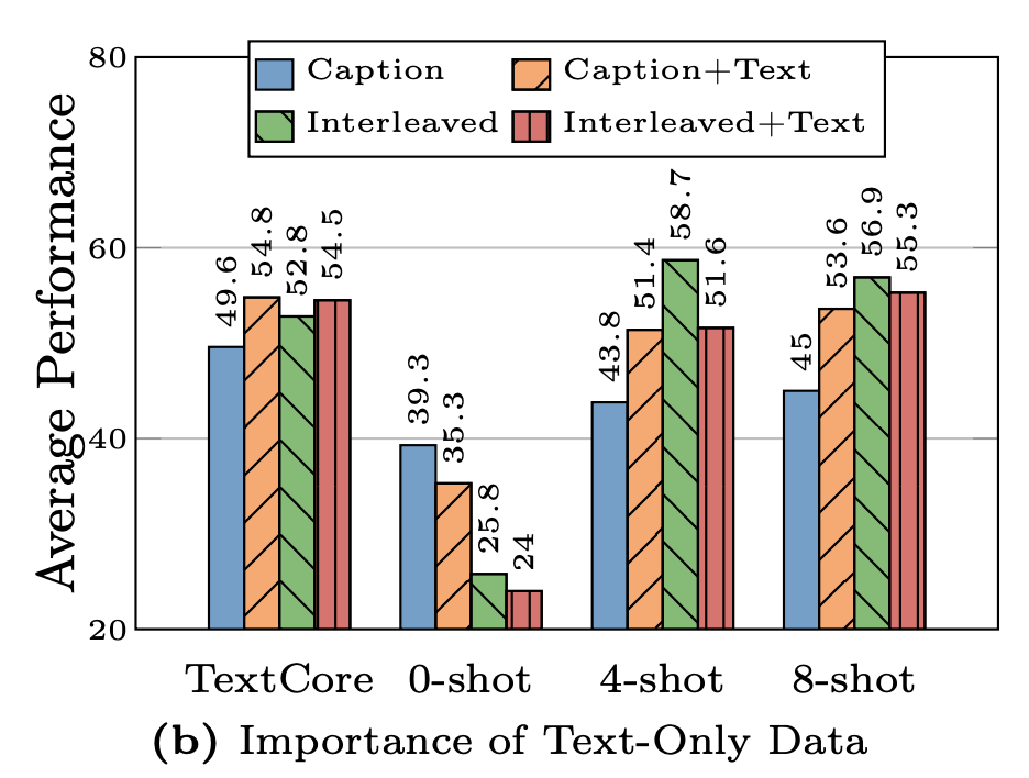
Second, Text-only data helps with few-shot reasoning. Text-only in this context means that the training data includes image examples and text-only examples. This was done to ensure that the model understands human language as well as images. Comparing the caption-only to caption-with-text shows a marked improvement for all but the 0-shot reasoning, however, interleaved-only performs better than interleaved-plus-text for all but the TextCore test.

Third, if you get the mixture right between image and text you can get really strong performance. The above graph shows different ratios of interleaved + captioned data to text-only data. As the goal is to have a multi-modal model, they never tested the performance if you do not have any image data. The authors here point out that the 91/9 ratio produced the most consistently good results.
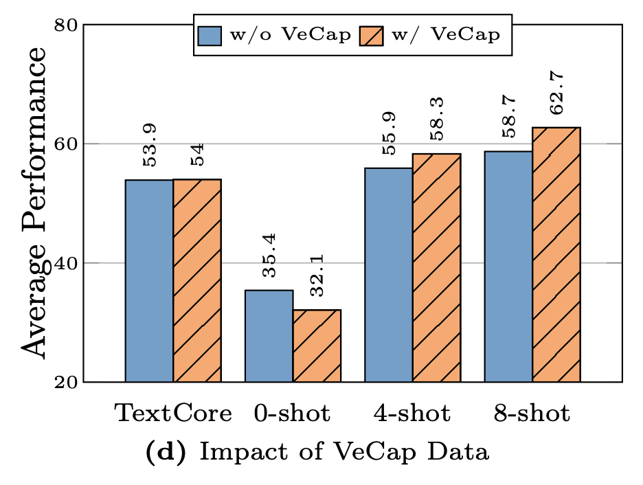
Fourth, synthetic data helps with few-shot learning. VeCap stands for Visual-enriched Caption, which is a way of creating captions so that they are sure to describe key visual pieces of the image. For the reverse, imagine a caption that may explain the meaning behind a photo but doesn’t explain any of the elements in the photo. You would typically do this if your data-scraper found images with poor alt-text data.
The authors here concluded that VeCap gives a “non-trivial” boost in few-shot reasoning, but has a relatively small increase in quality. This raises questions about the cost-effectiveness of VeCap.
Using the results from their ablations, the authors created a Transformer in two-forms: Mixture-of-Expert and regular. Both models had an encoder with a 378 x 378 image, pre-trained with DFN-5B dataset only. They had a mix of 45% captioned data, 45% interleaved data, and 10% text-only data (approximating the 91:9 ratio of image to text data). The VL Connector had 144 tokens and they chose a C Abstractor, though they point out that this was a somewhat arbitrary choice. For the LLM itself, they created a 3B, 7B, and 30B parameter model (with the MoE model only going up to 7B). The graph below shows how the these models performed.
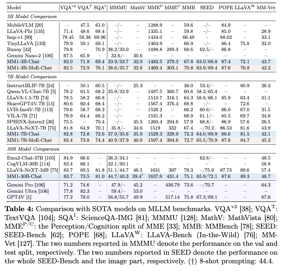
Interestingly, the 30B parameter model performs on par with other models which have billions more parameters than it (LLaVA-NeXT-34B, etc.), suggesting that there may be some quantum relationship between parameter size and performance here.
Multi-modal LLMs are an incredibly exciting part of the field. As we find better ways to transmit different data types into tokens, we may unlock even greater applications for these transformers. As we look to the future, it is not unreasonable now to consider how other senses could be inputed outside of a text description, such as sound, smell, or even touch. Data quality is likely to only become more valuable.
As the authors concluded that the different language connectors don’t make a major difference, it will be interesting to see if this means research should focus on the image encoder, or rather if we simply haven’t found a true breakthrough way to use the VL connector.
Outside of this specific paper, one of the big questions that arises is how these MLLMs will perform outside of benchmarks. As LLMs have proliferated, one common criticism revolves around the use of benchmarks to compare them. Often times these benchmarks use a consistent dataset to compare, allowing one model to do better simply by overfitting, even if unintentionally. Using methodologies like ELO, the chess rating algorithm, in the LLM Arena from lmsys may give a better true comparison of model performance.
In closing, as more inputs are able to be connected to LLMs, one can expect that the number of applications they can be applied to will increase. Only time will tell how useful we can make this technology.
[1] McKinzie, B., et al. “MM1: Methods, Analysis & Insights from Multimodal LLM Pre-training” (2024), arXiv
[2] Cha, J., et al. “Honeybee: Locality-enhanced Projector for Multimodal LLM” (2023), arXiv
[3] Antoniadis, P., et al. “Machine Learning: What Is Ablation Study?” (2024), arXiv
[4] Radford, A., et al. “Learning Transferable Visual Models From Natural Language Supervision” (2021), arXiv
[5] El-Nouby, Al., et al. “Scalable Pre-training of Large Autoregressive Image Models” (2024), arXiv
[6] Vaswani, A., et al., “Attention Is All You Need” (2017), arXiv
[7] Lai, Z., et al., “VeCLIP: Improving CLIP Training via Visual-enriched Captions” (2023), arXiv
Multimodal Large Language Models & Apple’s MM1 was originally published in Towards Data Science on Medium, where people are continuing the conversation by highlighting and responding to this story.