Tag: AI

The art of getting quick gains with agile model production

This post was written together with and inspired by Yuval Cohen

Introduction

Every day, numerous data science projects are discarded due to insufficient prediction accuracy. It’s a regrettable outcome, considering that often these models could be exceptionally well-suited for some subsets of the dataset.

Data Scientists often try to improve their models by using more complex models and by throwing more and more data at the problem. But many times there is a much simpler and more productive approach: Instead of trying to make all of our predictions better all at once, we could start by making good predictions for the easy parts of the data, and only then work on the harder parts.

This approach can greatly affect our ability to solve real-world problems. We start with the quick gain on the easy problems and only then focus our effort on the harder problems.

Thinking Agile

Agile production means focusing on the easy data first, and only after it has been properly modelled, moving on the the more complicated tasks. This allows a workflow that is iterative, value-driven, and collaborative.

It allows for quicker results, adaptability to changing circumstances, and continuous improvement, which are core ideas of agile production.

1. Iterative and incremental approach: work in short, iterative cycles. Start by achieving high accuracy for the easy problems and then move on to the harder parts.
2. Focus on delivering value: work on the problem with the highest marginal value for your time.
3. Flexibility and adaptability: Allow yourself to adapt to changing circumstances. For example, a client might need you to focus on a certain subset of the data — once you’ve solved that small problem, the circumstances have changed and you might need to work on something completely different. Breaking the problem into small parts allows you to adapt to the changing circumstances.
4. Feedback and continuous improvement: By breaking up a problem you allow yourself to be in constant and continuous improvement, rather than waiting for big improvements in large chunks.
5. Collaboration: Breaking the problem into small pieces promotes parallelization of the work and collaboration between team members, rather than putting all of the work on one person.

Breaking down the complexity

In real-world datasets, complexity is the rule rather than the exception. Consider a medical diagnosis task, where subtle variations in symptoms can make the difference between life-threatening conditions and minor ailments. Achieving high accuracy in such scenarios can be challenging, if not impossible, due to the inherent noise and nuances in the data.

This is where the idea of coverage comes into play. Coverage refers to the portion of the data that a model successfully predicts or classifies with high confidence or high precision. Instead of striving for high accuracy across the entire dataset, researchers can choose to focus on a subset of the data where prediction is relatively straightforward. By doing so, they can achieve high accuracy on this subset while acknowledging the existence of a more challenging, uncovered portion.

For instance, consider a trained model with a 50% accuracy rate on a test dataset. In this scenario, it’s possible that if we could identify and select only the predictions we are very sure about (although we should decide what “very sure” means), we could end up with a model that covers fewer cases, let’s say around 60%, but with significantly improved accuracy, perhaps reaching 85%.

I don’t know any product manager who would say no in such a situation. Especially if there is no model in production, and this is the first model.

The two-step model

We want to divide our data into two distinct subsets: the covered and the uncovered. The covered data is the part of the data where the initial model achieves high accuracy and confidence. The uncovered data is the part of the data where our model does not give confident predictions and does not achieve high accuracy.

In the first step, a model is trained on the data. Once we identify a subset of data where the model achieves high accuracy, we deploy that model and let it run on that subset — the covered data.

In the second step, we move our focus to the uncovered data. We try to develop a better model for this data by collecting more data, using more advanced algorithms, feature engineering, and incorporating domain-specific knowledge to find patterns in the data.

At this step, the first thing you should do is look at the errors by eye. Many times you will easily identify many patterns this way before using any fancy tricks.

An example

This example will show how the concept of agile workflow can create great value. This is a very simple example that is meant to visualize this concept. Real-life examples will be a lot less obvious but the idea that you will see here is just as relevant.

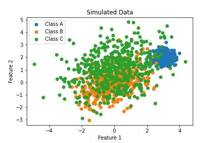
Let’s look at this two-dimensional data that I simulated from three equally sized classes.

num_samples_A = 500
num_samples_B = 500
num_samples_C = 500


# Class A
mean_A = [3, 2]
cov_A = [[0.1, 0], [0, 0.1]]  # Low variance
class_A = np.random.multivariate_normal(mean_A, cov_A, num_samples_A)

# Class B
mean_B = [0, 0]
cov_B = [[1, 0.5], [0.5, 1]]  # Larger variance with some overlap with class C
class_B = np.random.multivariate_normal(mean_B, cov_B, num_samples_B)

# Class C
mean_C = [0, 1]
cov_C = [[2, 0.5], [0.5, 2]]  # Larger variance with some overlap with class B
class_C = np.random.multivariate_normal(mean_C, cov_C, num_samples_C)

Now we try to fit a machine learning classifier to this data, it looks like an SVM classifier with a Gaussian (‘rbf’) kernel might do the trick:

import pandas as pd
from sklearn.model_selection import train_test_split
from sklearn.linear_model import LogisticRegression
from sklearn.svm import SVC

# Creating DataFrame
data = np.concatenate([class_A, class_B, class_C])
labels = np.concatenate([np.zeros(num_samples_A), np.ones(num_samples_B), np.ones(num_samples_C) * 2])
df = pd.DataFrame(data, columns=['x', 'y'])
df['label'] = labels.astype(int)

# Splitting data into train and test sets
X_train, X_test, y_train, y_test = train_test_split(df[['x', 'y']], df['label'], test_size=0.2, random_state=42)

# Training SVM model with RBF kernel
svm_rbf = SVC(kernel='rbf', probability= True)
svm_rbf.fit(X_train, y_train)

# Predict probabilities for each class
svm_rbf_probs = svm_rbf.predict_proba(X_test)

# Get predicted classes and corresponding confidences
svm_rbf_predictions = [(X_test.iloc[i]['x'], X_test.iloc[i]['y'], true_class, np.argmax(probs), np.max(probs)) for i, (true_class, probs) in enumerate(zip(y_test, svm_rbf_probs))]

svm_predictions_df = pd.DataFrame(svm_rbf_predictions).rename(columns={0:'x',1:'y' ,2: 'true_class', 3: 'predicted_class', 4: 'confidence'})

How does this model perform on our data?

accuracy = (svm_predictions_df['true_class'] == svm_predictions_df['predicted_class']).mean()*100
print(f'Accuracy = {round(accuracy,2)}%')

Accuracy = 75.33%

75% percent accuracy is disappointing, but does this mean that this model is useless?

Now we want to look at the most confident predictions and see how the model performs on them. How do we define the most confident predictions? We can try out different confidence (predict_proba) thresholds and see what coverage and accuracy we get for each threshold and then decide which threshold meets our business needs.

thresholds = [.5, .55, .6, .65, .7, .75, .8, .85, .9]
results = []

for threshold in thresholds:
    svm_df_covered = svm_predictions_df.loc[svm_predictions_df['confidence'] > threshold]
    coverage = len(svm_df_covered) / len(svm_predictions_df) * 100
    accuracy_covered = (svm_df_covered['true_class'] == svm_df_covered['predicted_class']).mean() * 100

    results.append({'Threshold': threshold, 'Coverage (%)': round(coverage,2), 'Accuracy on covered data (%)': round(accuracy_covered,2)})

results_df = pd.DataFrame(results)
print(results_df)

And we get

Or if we want a more detailed look we can create a plot of the coverage and accuracy by threshold:

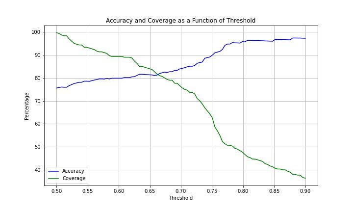
We can now select the threshold that fits our business logic. For example, if our company’s policy is to guarantee at least 90% accuracy, then we can choose a threshold of 0.75 and get an accuracy of 90% for 62% of the data. This is a huge improvement to throwing out the model, especially if we don’t have any model in production!

Now that our model is happily working in production on 60% of the data, we can shift our focus to the rest of the data. We can collect more data, do more feature engineering, try more complex models, or get help from a domain expert.

Balancing act

The two-step model allows us to aim for accuracy while acknowledging that it is perfectly fine to start with a high accuracy for only a subset of the data. It is counterproductive to insist that a model will have high accuracy on all the data before deploying it to production.

The agile approach presented in this post aims for resource allocation and efficiency. Instead of spending computational resources on getting high accuracy all across. Focus your resources on where the marginal gain is highest.

Conclusion

In data science, we try to achieve high accuracy. However, in the reality of messy data, we need to find a clever approach to utilize our resources in the best way. Agile model production teaches us to focus on the parts of the data where our model works best, deploy the model for those subsets, and only then start working on a new model for the more complicated part. This strategy will help you make the best use of your resources in the face of real data science problems.

Think production, Think Agile.

---

Coverage vs. Accuracy: Striking a Balance in Data Science was originally published in Towards Data Science on Medium, where people are continuing the conversation by highlighting and responding to this story.

In this post, we explore the performance benefits of Amazon SageMaker (including SMP and SMDDP), and how you can use the library to train large models efficiently on SageMaker. We demonstrate the performance of SageMaker with benchmarks on ml.p4d.24xlarge clusters up to 128 instances, and FSDP mixed precision with bfloat16 for the Llama 2 model.

Amazon Lex is a fully managed artificial intelligence (AI) service with advanced natural language models to design, build, test, and deploy conversational interfaces in applications. It employs advanced deep learning technologies to understand user input, enabling developers to create chatbots, virtual assistants, and other applications that can interact with users in natural language. Managing your […]

Generative artificial intelligence (AI) is transforming the customer experience in industries across the globe. Customers are building generative AI applications using large language models (LLMs) and other foundation models (FMs), which enhance customer experiences, transform operations, improve employee productivity, and create new revenue channels. The biggest concern we hear from customers as they explore the advantages of generative AI is how to protect their highly sensitive data and investments. At AWS, our top priority is safeguarding the security and confidentiality of our customers’ workloads. We think about security across the three layers of our generative AI stack …

The Practical Limitations and Advantages of Retrieval Augmented Generation (RAG)

The Value of RAG

Imagine RAG as highly intelligent librarian who can sift through a digital library in seconds to answer your questions. Sometimes the librarian finds relevant and useful information to answer your questions , but other times they miss the mark.

Let’s explore situations in which RAG excels and those in which it falls short. In a future work, I will explore a series of approaches that can be used individually or in combination to improve RAGs capabilities — which will support better responses when used with a language model.

Where RAG Falls Short

Even the most intelligent librarian has their challenges , some of which include the ability to reason iteratively, ensuring that they are retrieving the most useful documents, and ensure that the information they are sourcing from is relevant and unbiased.

Piecing Together the Puzzle with Iterative Reasoning: One of the key limitations of current RAG is its lack of iterative reasoning capabilities. RAG is unable to fully understand whether the data that is being retrieved is the most relevant information the language model needs to effectively solve the problem.

For example, if you were to pose a question such as “What does the impact of new environmental regulations passed in 2024 have on my latest white paper?” a RAG-enabled system would attempt to retrieve the data most semantically similar to the query. It might return the top X documents that have information on new policies, but are they the relevant policies for the specific paper the user is referencing?

As humans, we would approach this problem with reasoning skills. We would first read the white paper to understand its content and then determine what type of environmental policies best apply. Then based on that knowledge we would perform a search for those white papers. This iterative reasoning process — understanding the problem, formulating a more targeted search strategy, and then retrieving the most useful information — is a capability that current RAG implementations lack.

Organization Matters: The performance and effectiveness of RAG is heavily dependent on the organization and structure of the underlying data it is accessing. The ability for the retrieval algorithm to identify and surface the most useful documents is greatly influenced by how that information is cataloged and stored as well as how semantically similar the query is to the data retrieved.

In our library analogy, imagine a scenario where 500 books on various subjects are simply placed haphazardly on a single shelf, without any categorization or tagging. Trying to find the most relevant resources to answer a specific query would be a feat. You may stumble across some potentially useful books, but have no reliable way to assess which ones contain the most pertinent information. If those same 500 books were organized by genre, with clear metadata and subject tags, the retrieval process becomes significantly more efficient and effective. Rather than blindly scanning the entire shelf, the RAG implementation could quickly zero in on the most relevant section(s).

The same principles apply to how data is stored and indexed for RAG implementations in real-world applications. If the underlying datasets lack coherent organization, categorization, and metadata, the retrieval algorithms will struggle to identify the most valuable information. Ensuring data is properly structured, cataloged, and accessible is a critical.

The Good, the Bad, and the Biased : The quality of the data retrieved by a RAG implementation is only as good as the data it has access to. If the information in the underlying source systems, be it databases, online file storage, or other data repositories, contains outdated, incomplete, or biased content, the RAG implementation will have no way to discern this. It will simply retrieve and pass along this flawed information to the language model responsible for generating the final output.

Where RAG Models Shine

Accessing Domain Specific and Confidential Information: One of the key advantages of RAG is the ability to leverage domain-specific and even confidential information that may not be included in a language model’s standard training data. This can be particularly beneficial for organizations working on proprietary, cutting-edge research and projects. For example, if a company is conducting groundbreaking research in quantum computing that has not yet been publicly released, a RAG implementation could be granted access to these internal data sources. This would allow the language model to access specialized knowledge to engage in discussions about the company’s latest developments, without needing to be trained on that confidential information.

However, exposing sensitive, internal data to externally hosted language models (such as GPT, LLAMA, etc.) is not risk free. Organizations must exercise due diligence to ensure proper data security measures are in place to protect their intellectual property and confidential information.

Bringing the Latest News to Your Conversation: One of the key advantages of RAG is its ability to provide language models with access to the most up-to-date information, going beyond the fixed cutoff date of the language model’s original training data.If a language model were to rely solely on its inherent knowledge, its information would be limited to what was available at the time it was trained.

RAG implementations, on the other hand, can be integrated with live data sources such as the internet, constantly updating databases, news feeds, etc. This allows the language model to utilize current information when generating responses.

Conclusion

Retrieval Augmented Generation (RAG) is a powerful technique that can enhance language models by providing access to a wealth of information beyond their initial training. However, it is important to be aware of the limitations of RAG, such as the need for iterative reasoning, the importance of well organized data, and the potential for biased or outdated information. In a future work, I will explore a series of approaches to improve the capabilities of RAG — enhancing the quality of responses generated by a language model.

---

The Limitations and Advantages of Retrieval Augmented Generation (RAG) was originally published in Towards Data Science on Medium, where people are continuing the conversation by highlighting and responding to this story.

Deploying Large Language Models: vLLM and Quantization

Step-by-step guide on how to accelerate large language models

Deployment of Large Language Models (LLMs)

We live in an amazing time of Large Language Models like ChatGPT, GPT-4, and Claude that can perform multiple amazing tasks. In practically every field, ranging from education, healthcare to arts and business, Large Language Models are being used to facilitate efficiency in delivering services. Over the past year, many brilliant open-source Large Language Models, such as Llama, Mistral, Falcon, and Gemma, have been released. These open-source LLMs are available for everyone to use, but deploying them can be very challenging as they can be very slow and require a lot of GPU compute power to run for real-time deployment. Different tools and approaches have been created to simplify the deployment of Large Language Models.

Many deployment tools have been created for serving LLMs with faster inference, such as vLLM, c2translate, TensorRT-LLM, and llama.cpp. Quantization techniques are also used to optimize GPUs for loading very large Language Models. In this article, I will explain how to deploy Large Language Models with vLLM and quantization.

Latency and Throughput

Some of the major factors that affect the speed performance of a Large Language Model are GPU hardware requirements and model size. The larger the size of the model, the more GPU compute power is required to run it. Common benchmark metrics used in measuring the speed performance of a Large Language Model are Latency and Throughput.

Latency: This is the time required for a Large Language Model to generate a response. It is usually measured in seconds or milliseconds.

Throughput: This is the number of tokens generated per second or millisecond from a Large Language Model.

Install Required Packages

Below are the two required packages for running a Large Language Model: Hugging Face transformers and accelerate.

pip3 install transformers
pip3 install accelerate

What is Phi-2?

Phi-2 is a state-of-the-art foundation model from Microsoft with 2.7 billion parameters. It was pre-trained with a variety of data sources, ranging from code to textbooks. Learn more about Phi-2 from here.

Benchmarking LLM Latency and Throughput with Hugging Face Transformers

Generated Output

Latency: 2.739394464492798 seconds
Throughput: 32.36171766303386 tokens/second
Generate a python code that accepts a list of numbers and returns the sum. [1, 2, 3, 4, 5]
A: def sum_list(numbers):
    total = 0
    for num in numbers:
        total += num
    return total

print(sum_list([1, 2, 3, 4, 5]))

Step By Step Code Breakdown

Line 6–10: Loaded Phi-2 model and tokenized the prompt “Generate a python code that accepts a list of numbers and returns the sum.”

Line 12- 18: Generated a response from the model and obtained the latency by calculating the time required to generate the response.

Line 21–23: Obtained the total length of tokens in the response generated, divided it by the latency and calculated the throughput.

This model was run on an A1000 (16GB GPU), and it achieves a latency of 2.7 seconds and a throughput of 32 tokens/second.

Deployment of A Large Language Model with vLLM

vLLM is an open source LLM library for serving Large Language Models at low latency and high throughput.

How vLLM works

The transformer is the building block of Large Language Models. The transformer network uses a mechanism called the attention mechanism, which is used by the network to study and understand the context of words. The attention mechanism is made up of a bunch of mathematical calculations of matrices known as attention keys and values. The memory used by the interaction of these attention keys and values affects the speed of the model. vLLM introduced a new attention mechanism called PagedAttention that efficiently manages the allocation of memory for the transformer’s attention keys and values during the generation of tokens. The memory efficiency of vLLM has proven very useful in running Large Language Models at low latency and high throughput.

This is a high-level explanation of how vLLM works. To learn more in-depth technical details, visit the vLLM documentation.

vLLM: Easy, Fast, and Cheap LLM Serving with PagedAttention

Install vLLM

pip3 install vllm==0.3.3

Run Phi-2 with vLLM

Generated Output

Latency: 1.218436622619629seconds
Throughput: 63.15334836428132tokens/second
 [1, 2, 3, 4, 5]
A: def sum_list(numbers):
    total = 0
    for num in numbers:
        total += num
    return total

numbers = [1, 2, 3, 4, 5]
print(sum_list(numbers))

Step By Step Code Breakdown

Line 1–3: Imported required packages from vLLM for running Phi-2.

Line 5–8: Loaded Phi-2 with vLLM, defined the prompt and set important parameters for running the model.

Line 10–16: Generated the model’s response using llm.generate and computed the latency.

Line 19–21: Obtained the length of total tokens generated from the response, divided the length of tokens by the latency to get the throughput.

Line 23–24: Obtained the generated text.

I ran Phi-2 with vLLM on the same prompt, “Generate a python code that accepts a list of numbers and returns the sum.” On the same GPU, an A1000 (16GB GPU), vLLM produces a latency of 1.2 seconds and a throughput of 63 tokens/second, compared to Hugging Face transformers’ latency of 2.85 seconds and a throughput of 32 tokens/second. Running a Large Language Model with vLLM produces the same accurate result as using Hugging Face, with much lower latency and higher throughput.

Note: The metrics (latency and throughput) I obtained for vLLM are estimated benchmarks for vLLM performance. The model generation speed depends on many factors, such as the length of the input prompt and the size of the GPU. According to the official vLLM report, running an LLM model on a powerful GPU like the A100 in a production setting with vLLM achieves 24x higher throughput than Hugging Face Transformers.

Benchmarking Latency and Throughput in Real Time

The way I calculated the latency and throughput for running Phi-2 is experimental, and I did this to explain how vLLM accelerates a Large Language Model’s performance. In the real-world use case of LLMs, such as a chat-based system where the model outputs a token as it is generated, measuring the latency and throughput is more complex.

A chat-based system is based on streaming output tokens. Some of the major factors that affect the LLM metrics are Time to First Token (the time required for a model to generate the first token), Time Per Output Token (the time spent per output token generated), the input sequence length, the expected output, the total expected output tokens, and the model size. In a chat-based system, the latency is usually a combination of Time to First Token and Time Per Output Token multiplied by the total expected output tokens.

The longer the input sequence length passed into a model, the slower the response. Some of the approaches used in running LLMs in real-time involve batching users’ input requests or prompts to perform inference on the requests concurrently, which helps in improving the throughput. Generally, using a powerful GPU and serving LLMs with efficient tools like vLLM improves both the latency and throughput in real-time.

Run the vLLM deployment on Google Colab

Google Colaboratory

Quantization of Large Language Models

Quantization is the conversion of a machine learning model from a higher precision to a lower precision by shrinking the model’s weights into smaller bits, usually 8-bit or 4-bit. Deployment tools like vLLM are very useful for inference serving of Large Language Models at very low latency and high throughput. We are able to run Phi-2 with Hugging Face and vLLM conveniently on the T4 GPU on Google Colab because it is a smaller LLM with 2.7 billion parameters. For example, a 7-billion-parameter model like Mistral 7B cannot be run on Colab with either Hugging Face or vLLM. Quantization is best for managing GPU hardware requirements for Large Language Models. When GPU availability is limited and we need to run a very large Language Model, quantization is the best approach to load LLMs on constrained devices.

BitsandBytes

It is a python library built with custom quantization functions for shrinking model’s weights into lower bits(8-bit and 4-bit).

Install BitsandBytes

pip3 install bitsandbytes

Quantization of Mistral 7B Model

Mistral 7B, a 7-billion-parameter model from MistralAI, is one of the best state-of-the-art open-source Large Language Models. I will go through a step-by-step process of running Mistral 7B with different quantization techniques that can be run on the T4 GPU on Google Colab.

Quantization with 8bit Precision: This is the conversion of a machine learning model’s weight into 8-bit precision. BitsandBytes has been integrated with Hugging Face transformers to load a language model using the same Hugging Face code, but with minor modifications for quantization.

Line 1: Imported the needed packages for running model, including the BitsandBytesConfig library.

Line 3–4: Defined the quantization config and set the parameter load_in_8bit to true for loading the model’s weights in 8-bit precision.

Line 7–9: Passed the quantization config into the function for loading the model, set the parameter device_map for bitsandbytes to automatically allocate appropriate GPU memory for loading the model. Finally loaded the tokenizer weights.

Quantization with 4bit Precision: This is the conversion of a machine learning model’s weight into 4-bit precision.

The code for loading Mistral 7B in 4-bit precision is similar to that of 8-bit precision except for a few changes:

• changed load_in_8bit to load_in_4bit.
• A new parameter bnb_4bit_compute_dtype is introduced into the BitsandBytesConfig to perform the model’s computation in bfloat16. bfloat16 is computation data type for loading model’s weights for faster inference. It can be used with both 4-bit and 8-bit precisions. If it is in 8-bit you just need to change the parameter from bnb_4bit_compute_dtype to bnb_8bit_compute_dtype.

NF4(4-bit Normal Float) and Double Quantization

NF4 (4-bit Normal Float) from QLoRA is an optimal quantization approach that yields better results than the standard 4-bit quantization. It is integrated with double quantization, where quantization occurs twice; quantized weights from the first stage of quantization are passed into the next stage of quantization, yielding optimal float range values for the model’s weights. According to the report from the QLoRA paper, NF4 with double quantization does not suffer from a drop in accuracy performance. Read more in-depth technical details about NF4 and Double Quantization from the QLoRA paper:

QLoRA: Efficient Finetuning of Quantized LLMs

Line 4–9: Extra parameters were set the BitsandBytesConfig:

• load_4bit: loading model in 4-bit precision is set to true.
• bnb_4bit_quant_type: The type of quantization is set to nf4.
• bnb_4bit_use_double_quant: Double quantization is set to True.
• bnb_4_bit_compute_dtype: bfloat16 computation data type is used for faster inference.

Line 11–13: Loaded the model’s weights and tokenizer.

Full Code for Model Quantization

Generated Output

<s> [INST] What is Natural Language Processing? [/INST] Natural Language Processing (NLP) is a subfield of artificial intelligence (AI) and
computer science that deals with the interaction between computers and human language. Its main objective is to read, decipher, 
understand, and make sense of the human language in a valuable way. It can be used for various tasks such as speech recognition, 
text-to-speech synthesis, sentiment analysis, machine translation, part-of-speech tagging, name entity recognition, 
summarization, and question-answering systems. NLP technology allows machines to recognize, understand,
 and respond to human language in a more natural and intuitive way, making interactions more accessible and efficient.</s>

Quantization is a very good approach for optimizing the running of very Large Language Models on smaller GPUs and can be applied to any model, such as Llama 70B, Falcon 40B, and mpt-30b. According to reports from the LLM.int8 paper, very Large Language Models suffer less from accuracy drops when quantized compared to smaller ones. Quantization is best applied to very Large Language Models and does not work well for smaller models because of the loss in accuracy performance.

Run Mixtral 7B Quantization on Google Colab

Google Colaboratory

Conclusion

In this article, I provided a step-by-step approach to measuring the speed performance of a Large Language Model, explained how vLLM works, and how it can be used to improve the latency and throughput of a Large Language Model. Finally, I explained quantization and how it is used to load Large Language Models on small-scale GPUs.

Reach to me via:

Email: [email protected]

Linkedin: https://www.linkedin.com/in/ayoola-olafenwa-003b901a9/

References

• vLLM: Easy, Fast, and Cheap LLM Serving with PagedAttention
• Making LLMs even more accessible with bitsandbytes, 4-bit quantization and QLoRA
• Understanding performance benchmarks for LLM inference
• What are Quantized LLMs?

---

Deploying Large Language Models: vLLM and QuantizationStep by Step Guide on How to Accelerate… was originally published in Towards Data Science on Medium, where people are continuing the conversation by highlighting and responding to this story.

References

[1] Abadie, Alberto, and Jaume Vives-i-Bastida. “Synthetic controls in action.” arXiv preprint arXiv:2203.06279 (2022).
[2]Brodersen, Kay H., et al. “Inferring causal impact using Bayesian structural time-series models.” (2015): 247–274.
[3]https://medium.com/@dreamferus/how-to-synchronize-time-series-using-cross-correlation-in-python-4c1fd5668c7a
[4]Abadie, Alberto, and Jinglong Zhao. “Synthetic controls for experimental design.” arXiv preprint arXiv:2108.02196 (2021).
Towards Reliable Synthetic Control was originally published in Towards Data Science on Medium, where people are continuing the conversation by highlighting and responding to this story.
Originally appeared here:
Towards Reliable Synthetic Control
Go Here to Read this Fast! Towards Reliable Synthetic Control