This post walks you through the Open Source Observability pattern for AWS Inferentia, which shows you how to monitor the performance of ML chips, used in an Amazon Elastic Kubernetes Service (Amazon EKS) cluster, with data plane nodes based on Amazon Elastic Compute Cloud (Amazon EC2) instances of type Inf1 and Inf2.
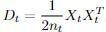
With the rise of the transformer architecture and high-throughput compute, training foundational models has turned into a hot topic recently. This has led to promising efforts to either integrate or train foundational models to enhance the capabilities of reinforcement learning (RL) algorithms, signaling an exciting direction for the field. Here, we’re discussing how foundational models can give reinforcement learning a major boost.
Before diving into the latest research on how foundational models can give reinforcement learning a major boost, let’s engage in a brainstorming session. Our goal is to pinpoint areas where pre-trained foundational models, particularly Large Language Models (LLMs) or Vision-Language Models (VLMs), could assist us, or how we might train a foundational model from scratch. A useful approach is to examine each element of the reinforcement learning training loop individually, to identify where there might be room for improvement:
Fig 1: Overview of foundation models in RL (Image by author)
1- Environment: Given that pre-trained foundational models understand the causal relationships between events, they can be utilized to forecast environmental changes resulting from current actions. Although this concept is intriguing, we’re not yet aware of any specific studies that focus on it. There are two primary reasons holding us back from exploring this idea further for now.
While the reinforcement learning training process demands highly accurate predictions for the next step observations, pre-trained LLMs/VLMs haven’t been directly trained on datasets that enable such precise forecasting and thus fall short in this aspect. It’s important to note, as we highlighted in our previous post, that a high-level planner, particularly one used in lifelong learning scenarios, could effectively incorporate a foundational model.
Latency in environment steps is a critical factor that can constrain the RL algorithm, especially when working within a fixed budget for training steps. The presence of a very large model that introduces significant latency can be quite restrictive. Note that while it might be challenging, distillation into a smaller network can be a solution here.
2- State (LLM/VLM Based State Generator): While experts often use the terms observation and state interchangeably, there are distinctions between them. A state is a comprehensive representation of the environment, while an observation may only provide partial information. In the standard RL framework, we don’t often discuss the specific transformations that extract and merge useful features from observations, past actions, and any internal knowledge of the environment to produce “state”, the policy input. Such a transformation could be significantly enhanced by employing LLMs/VLMs, which allow us to infuse the “state” with broader knowledge of the world, physics, and history (refer to Fig. 1, highlighted in pink).
3- Policy (Foundational Policy Model): Integrating foundational models into the policy, the central decision-making component in RL, can be highly beneficial. Although employing such models to generate high-level plans has proven successful, transforming the state into low-level actions has challenges we’ll delve into later. Fortunately, there has been some promising research in this area recently.
4- Reward (LLM/VLM Based Reward Generator): Leveraging foundational models to more accurately assess chosen actions within a trajectory has been a primary focus among researchers. This comes as no surprise, given that rewards have traditionally served as the communication channel between humans and agents, setting goals and guiding the agent towards what is desired.
Pre-trained foundational models come with a deep knowledge of the world, and injecting this kind of understanding into our decision-making processes can make those decisions more in tune with human desires and more likely to succeed. Moreover, using foundational models to evaluate the agent’s actions can quickly trim down the search space and equip the agent with a head start in understanding, as opposed to starting from scratch.
Pre-trained foundational models have been trained on internet-scale data generated mostly by humans, which has enabled them to understand worlds similarly to humans. This makes it possible to use foundational models as cost-effective annotators. They can generate labels or assess trajectories or rollouts on a large scale.
1- Foundational models in reward
It is challenging to use foundational models to generate low level control actions as low level actions are highly dependent on the setting of the agent and are underrepresented in foundational models’ training dataset. Hence, the foundation model application is generally focused on high level plans rather than low level actions. Reward bridges the gap between high-level planner and low level actions where foundation models can be used. Researchers have adopted various methodologies integrating foundation models for reward assignment. However, the core principle revolves around employing a VLM/LLM to effectively track the progress towards a subgoal or task.
1.a Assigning reward values based on similarity
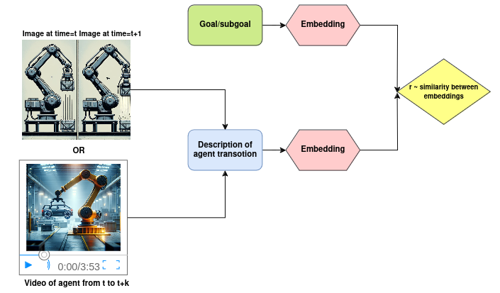
Consider the reward value as a signal that indicates whether the agent’s previous action was beneficial in moving towards the goal. A sensible method involves evaluating how closely the previous action aligns with the current objective. To put this approach into practice, as can be seen in Fig. 2, it’s essential to: – Generate meaningful embeddings of these actions, which can be done through images, videos, or text descriptions of the most recent observation. – Generate meaningful representations of the current objective. – Assess the similarity between these representations.
Fig 2. Reward values based on similarity (Image by author).
Let’s explore the specific mechanics behind the leading research in this area.
Dense and well-shaped reward functions enhance the stability and training speed of the RL agent. Intrinsic rewards address this challenge by rewarding the agent for novel states’ exploration. However, in large environments where most of the unseen states are irrelevant to the downstream task, this approach becomes less effective. ELLM uses background knowledge of LLM to shape the exploration. It queries LLM to generate a list of possible goals/subgoals given a list of the agent’s available actions and a text description of the agent current observation, generated by a state captioner. Then, at each time step, the reward is computed by the semantic similarity, cosine similarity, between the LLM generated goal and the description of the agent’s transition.
LiFT has a similar framework but also leverages CLIP4Clip-style VLMs for reward assignment. CLIP4Clip is pre-trained to align videos and corresponding language descriptions through contrastive learning. In LiFT, the agent is rewarded based on the alignment score, cosine similarity, between the task instructions and videos of the agent’s corresponding behavior, both encoded by CLIP4CLIP.
UAFM has a similar framework where the main focus is on robotic manipulation tasks, e.g., stacking a set of objects. For reward assignment, they measure the similarity between the agent state image and the task description, both embedded by CLIP. They finetune CLIP on a small amount of data from the simulated stacking domain to be more aligned in this use case.
1.b Assigning rewards through reasoning on auxiliary tasks:
In scenarios where the foundational model has the proper understanding of the environment, it becomes feasible to directly pass the observations within a trajectory to the model, LLM/VLM. This evaluation can be done either through straightforward QA sessions based on the observations or by verifying the model’s capability in predicting the goal only by looking at the observation trajectory.
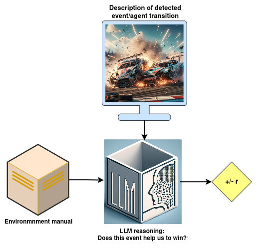
Fig 3. Assigning reward through reasoning (Image by author).
Read and Reward integrates the environment’s instruction manual into reward generation through two key components, as can be seen in Fig. 3:
QA extraction module: it creates a summary of game objectives and features. This LLM-based module, RoBERTa-large, takes in the game manual and a question, and extracts the corresponding answer from the text. Questions are focused on the game objective, and agent-object interaction, identified by their significance using TF-IDF. For each critical object, a question as: “What happens when the player hits a <object>?” is added to the question set. A summary is then formed with the concatenation of all non-empty question-answer pairs.
Reasoning module: During gameplay, a rule-based algorithm detects “hit” events. Following each “hit” event, the LLM based reasoning module is queried with the summary of the environment and a question: “Should you hit a <object of interaction> if you want to win?” where the possible answer is limited to {yes, no}. A “yes” response adds a positive reward, while “no” leads to a negative reward.
EAGER introduces a unique method for creating intrinsic rewards through a specially designed auxiliary task. This approach presents a novel concept where the auxiliary task involves predicting the goal based on the current observation. If the model predicts accurately, this indicates a strong alignment with the intended goal, and thus, a larger intrinsic reward is given based on the prediction confidence level. To achieve this goal, To accomplish this, two modules are employed:
Question Generation (QG): This component works by masking all nouns and adjectives in the detailed objective provided by the user.
Question Answering (QA): This is a model trained in a supervised manner, which takes the observation, question masks, and actions, and predicts the masked tokens.
(P.S. Although this work does not utilize a foundational model, we’ve included it here due to its intriguing approach, which can be easily adapted to any pre-trained LLM)
1.c Generating reward function code
Up to this point, we’ve discussed generating reward values directly for the reinforcement learning algorithms. However, running a large model at every step of the RL loop can significantly slow down the speed of both training and inference. To bypass this bottleneck, one strategy involves utilizing our foundational model to generate the code for the reward function. This allows for the direct generation of reward values at each step, streamlining the process.
For the code generation schema to work effectively, two key components are required: 1- A code generator, LLM, which receives a detailed prompt containing all the necessary information to craft the code. 2- A refinement process that evaluates and enhances the code in collaboration with the code generator. Let’s look at the key contributions for generating reward code:
R2R2S generates reward function code through two main components:
LLM based motion descriptor: This module uses a pre-defined template to describe robot movements, and leverages Large Language Models (LLMs) to understand the motion. The Motion Descriptor fills in the template, replacing placeholders e.g. “Destination Point Coordinate” with specific details, to describe the desired robot motion within a pre-defined template.
LLM based reward coder: this component generates the reward function by processing a prompt containing: a motion description, a list of functions with their description that LLM can use to generate the reward function code, an example code of how the response should look like, and constraints and rules the reward function must follow.
Text2Reward develops a method to generate dense reward functions as an executable code within iterative refinement. Given the subgoal of the task, it has two key components:
LLM-based reward coder: generates reward function code. Its prompt consists of: an abstract of observation and available actions, a compact pythonic style environment to represent the configuration of the objects, robot, and callable functions; a background knowledge for reward function design (e.g. “reward function for task X typically includes a term for the distance between object x and y”), and a few-shot examples. They assume access to a pool of instruction, and reward function pairs that top k similar instructions are retrieved as few-shot examples.
LLM-Based Refinement: once the reward code is generated, the code is executed to identify the syntax errors and runtime errors. These feedbacks are integrated into subsequent prompts to generate more refined reward functions. Additionally, human feedback is requested based on a task execution video by the current policy.
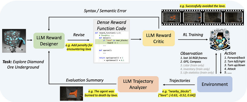
Auto MC-Reward has a similar algorithm to Text2Reward, to generate the reward function code, see Fig. 4. The main difference is in the refinement stage where it has two modules, both LLMs:
LLM-Based Reward Critic: It evaluates the code and provides feedback on whether the code is self-consistent and free of syntax and semantic errors.
LLM-Based Trajectory Analyser: It reviews the historical information of the interaction between the trained agent and the environment and uses it to guide the modifications of the reward function.
EUREKA generates reward code without the need for task-specific prompting, predefined reward templates, or predefined few-shot examples. To achieve this goal, it has two stages:
LLM-based code generation: The raw environment code, the task, generic reward design and formatting tips are fed to the LLM as context and LLM returns the executable reward code with a list of its components.
Evolutionary search and refinement: At each iteration, EUREKA queries the LLM to generate several i.i.d reward functions. Training an agent with executable reward functions provides feedback on how well the agent is performing. For a detailed and focused analysis of the rewards, the feedback also includes scalar values for each component of the reward function. The LLM takes top-performing reward code along with this detailed feedback to mutate the reward code in-context. In each subsequent iteration, the LLM uses the top reward code as a reference to generate K more i.i.d reward codes. This iterative optimization continues until a specified number of iterations has been reached.
Within these two steps, EUREKA is able to generate reward functions that outperform expert human-engineered rewards without any task specific templates.
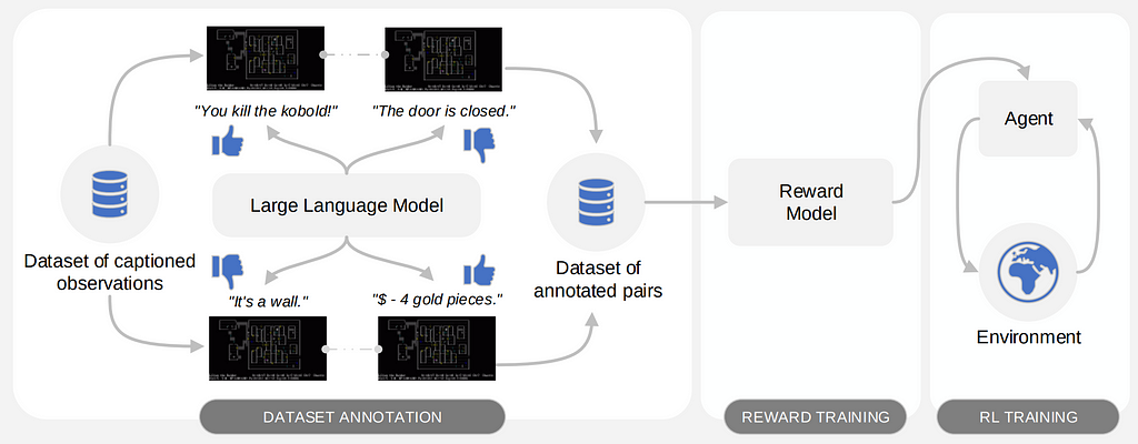
1.d. Train a reward model based on preferences (RLAIF)
An alternative method is to use a foundational model to generate data for training a reward function model. The significant successes of Reinforcement Learning with Human Feedback (RLHF) have recently drawn increased attention towards employing trained reward functions on a larger scale. The heart of such algorithms is the use of a preference dataset to train a reward model which can subsequently be integrated into reinforcement learning algorithms. Given the high cost associated with generating preference data (e.g., action A is preferable to action B) through human feedback, there’s growing interest in constructing this dataset by obtaining feedback from an AI agent, i.e. VLM/LLM. Training a reward function, using AI-generated data and integrating it within a reinforcement learning algorithm, is known as Reinforcement Learning with AI Feedback (RLAIF).
MOTIF requires access to a passive dataset of observations with sufficient coverage. Initially, LLM is queried with a summary of desired behaviors within the environment and a text description of two randomly sampled observations. It then generates the preference, selecting between 1, 2, or 0 (indicating no preference), as seen in Fig. 5. This process constructs a dataset of preferences between observation pairs. Subsequently, this dataset is used to train a reward model employing preference based RL techniques.
Fig 5. A schematic representation of the three phases of MOTIF (image taken from MOTIF paper)
2- Foundation models as Policy
Achieving the capability to train a foundational policy that not only excels in tasks previously encountered but also possesses the ability to reason about and adapt to new tasks using past learning, is an ambition within the RL community. Such a policy would ideally generalize from past experiences to tackle novel situations and, through environmental feedback, achieve goals previously unseen with human-like adaptability.
However, several challenges stand in the way of training such agents. Among these challenges are:
The necessity of managing a very large model, which introduces significant latency into the decision-making process for low-level control actions.
The requirement to collect a vast amount of interaction data across a wide array of tasks to enable effective learning.
Additionally, the process of training a very large network from scratch using RL introduces extra complexities. This is because backpropagation efficiency inherently is weaker in RL compared to supervised training methods .
Up to now, it’s mostly been teams with substantial resources and top-notch setups who’ve really pushed the envelope in this domain.
AdA paved the way for training an RL foundation model within the X.Land 2.0 3D environment. This model achieves human time-scale adaptation on held-out test tasks without any further training. The model’s success is founded on three ingredients:
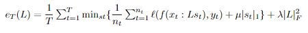
The core of the AdA’s learning mechanism is a Transformer-XL architecture from 23 to 265 million parameters, employed alongside the Muesli RL algorithm. Transformer-XL takes in a trajectory of observations, actions, and rewards from time t to T and outputs a sequence of hidden states for each time step. The hidden state is utilized to predict reward, value, and action distribution π. The combination of both long-term and short-term memory is critical for fast adaptation. Long-term memory is achieved through slow gradient updates, whereas short-term memory can be captured within the context length of the transformer. This unique combination allows the model to preserve knowledge across multiple task attempts by retaining memory across trials, even though the environment resets between trials.
The model benefits from meta-RL training across 1⁰⁴⁰ different partially observable Markov decision processes (POMDPs) tasks. Since transformers are meta-learners, no additional meta step is required.
Given the size and diversity of the task pool, many tasks will either be too easy or too hard to generate a good training signal. To tackle this, they used an automated curriculum to prioritize tasks that are within its capability frontier.
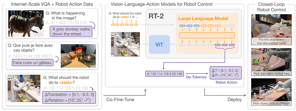
RT-2 introduces a method to co-finetune a VLM on both robotic trajectory data and vision-language tasks, resulting in a policy model called RT-2. To enable vision-language models to generate low-level actions, actions are discretized into 256 bins and represented as language tokens.
By representing actions as language tokens, RT-2 can directly utilize pre-existing VLM architectures without requiring substantial modifications. Hence, VLM input includes robot camera image and textual task description formatted similarly to Vision Question Answering tasks and the output is a series of language tokens that represent the robot’s low-level actions; see Fig. 6.
Fig 6. RT-2 overview (image taken from RT-2 paper)
They noticed that co-finetuning on both types of data with the original web data leads to more generalizable policies. The co-finetuning process equips RT-2 with the ability to understand and execute commands that were not explicitly present in its training data, showcasing remarkable adaptability. This approach enabled them to leverage internet-scale pretraining of VLM to generalize to novel tasks through semantic reasoning.
3- Foundation Models as State Representation
In RL, a policy’s understanding of the environment at any given moment comes from its “state” which is essentially how it perceives its surroundings. Looking at the RL block diagram, a reasonable module to inject world knowledge into is the state. If we can enrich observations with general knowledge useful for completing tasks, the policy can pick up new tasks much faster compared to RL agents that begin learning from scratch.
PR2L introduces a novel approach to inject the background knowledge of VLMs from internet scale data into RL.PR2L employs generative VLMs which generate language in response to an image and a text input. As VLMs are proficient in understanding and responding to visual and textual inputs, they can provide a rich source of semantic features from observations to be linked to actions.
PR2L, queries a VLM with a task-relevant prompt for each visual observation received by the agent, and receives both the generated textual response and the model’s intermediate representations. They discard the text and use some or all of the models intermediate representation generated for both the visual and text input and the VLM’s generated textual response as “promptable representations”. Due to the variable size of these representations, PR2L incorporates an encoder-decoder Transformer layer to embed all the information embedded in promptable representations into a fixed size embedding. This embedding, combined with any available non-visual observation data, is then provided to the policy network, representing the state of the agent. This innovative integration allows the RL agent to leverage the rich semantic understanding and background knowledge of VLMs, facilitating more rapid and informed learning of tasks.
[1] ELLM: Du, Yuqing, et al. “Guiding pretraining in reinforcement learning with large language models.” 2023. [2] Text2Reward: Xie, Tianbao, et al. “Text2reward: Automated dense reward function generation for reinforcement learning.” 2023. [3] R2R2S: Yu, Wenhao, et al. “Language to rewards for robotic skill synthesis.” 2023. [4] EUREKA: Ma, Yecheng Jason, et al. “Eureka: Human-level reward design via coding large language models.” 2023. [5] MOTIF: Klissarov, Martin, et al. “Motif: Intrinsic motivation from artificial intelligence feedback.” 2023. [6] Read and Reward: Wu, Yue, et al. “Read and reap the rewards: Learning to play atari with the help of instruction manuals.” 2024. [7] Auto MC-Reward: Li, Hao, et al. “Auto MC-reward: Automated dense reward design with large language models for minecraft.” 2023. [8] EAGER: Carta, Thomas, et al. “Eager: Asking and answering questions for automatic reward shaping in language-guided RL.” 2022. [9] LiFT: Nam, Taewook, et al. “LiFT: Unsupervised Reinforcement Learning with Foundation Models as Teachers.” 2023. [10] UAFM: Di Palo, Norman, et al. “Towards a unified agent with foundation models.” 2023. [11] RT-2: Brohan, Anthony, et al. “Rt-2: Vision-language-action models transfer web knowledge to robotic control.” 2023. [12] AdA: Team, Adaptive Agent, et al. “Human-timescale adaptation in an open-ended task space.” 2023. [13] PR2L: Chen, William, et al. “Vision-Language Models Provide Promptable Representations for Reinforcement Learning.” 2024. [14] Clip4Clip: Luo, Huaishao, et al. “Clip4clip: An empirical study of clip for end to end video clip retrieval and captioning.” 2022. [15] Clip: Radford, Alec, et al. “Learning transferable visual models from natural language supervision.” 2021. [16] RoBERTa: Liu, Yinhan, et al. “Roberta: A robustly optimized bert pretraining approach.” 2019. [17] Preference based RL: SWirth, Christian, et al. “A survey of preference-based reinforcement learning methods.” 2017. [18] Muesli: Hessel, Matteo, et al. “Muesli: Combining improvements in policy optimization.” 2021. [19] Melo, Luckeciano C. “Transformers are meta-reinforcement learners.” 2022. [20] RLHF: Ouyang, Long, et al. “Training language models to follow instructions with human feedback, 2022.
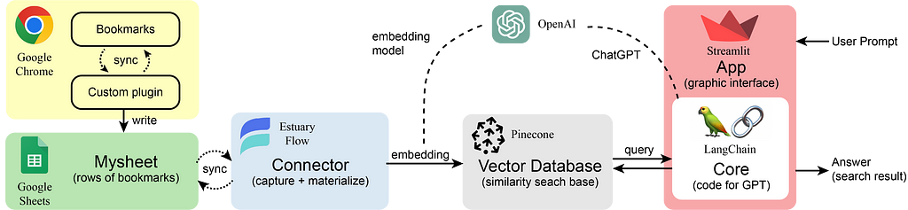
Let’s briefly remember what the 3 acronyms that make up the word RAG mean:
Retrieval: The main objective of a RAG is to collect the most relevant documents/chunks regarding the query.
Augmented: Create a well-structured prompt so that when the call is made to the LLM, it knows perfectly what its purpose is, what the context is and how it should respond.
Generation: This is where the LLM comes into play. When the model is given good context (provided by the “Retrieval” step) and has clear instructions (provided by the “Augmented” step), it will generate high-value responses for the user.
As we can see, the generation of the response to a user’s query (If we apply a RAG for the purpose of Q&A), depends directly on how well we have built the “Augmented” and especially the “Retrieval”.
In this article we are going to focus exclusively on the “Retrieval” part. In this important process of returning the most relevant documents, the concept of vector store appears.
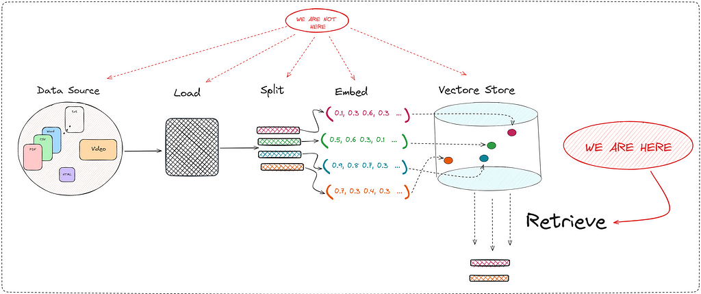
Overview of the techniques shown in this article (Image by Author).
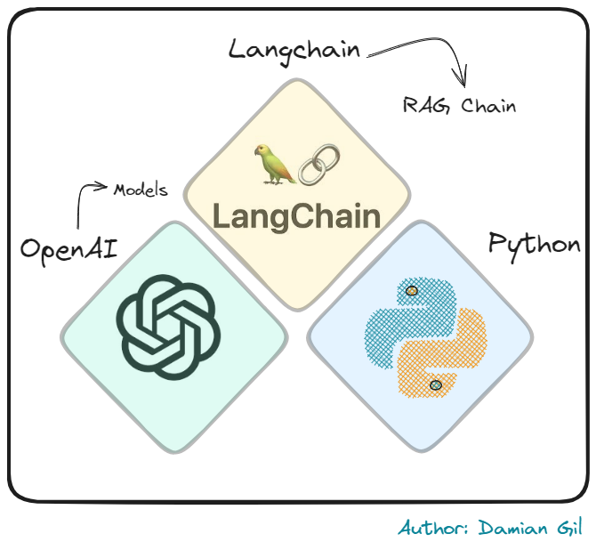
To create these retrievals, we will use the Langchain library.
Overview of the technologies used in this article (Image by Author).
The vectore store is nothing more than a vector database, which stores documents in vector format. This vector representation comes from the use of transformers. I’m not saying something you don’t know at the moment.
It is clear that the more robust and complete this vector store is, the better retriever we can run. We already know that the creation of this database is an art in itself. Depending on the size of the chunks or the embedding model we use, our RAG will be better or worse.
I make a clarification here:
In this post we are NOT going to discuss how to create this vector store. In this post we are going to discuss some of the techniques used to retrieve relevant documents.
Since a picture is worth a thousand words, I suggest you take a look at the following:
A RAG encompasses a series of well-defined steps. This post will only cover the retriever part (Image by Author).
Therefore, I reiterate that in this post we are going to deeply study one of the many important steps in creating a good RAG tool. The “Retrieve” step is key since it directly improves the context that the LLM has when generating a response.
The methods we will study are:
Naive Retriever
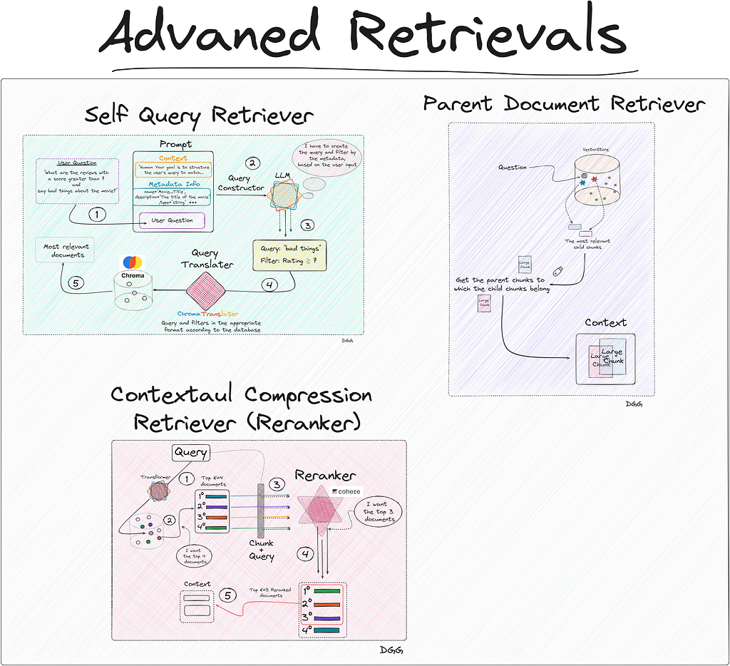
Parent Document Retriever
Self-Query Retriever
Contextual Compression Retriever (Reranking)
You can find the project with the notebooks here. And you can also take a look at my github:
To expose these methods, a practical use case will be carried out to improve the explanation. Therefore, we are going to create a RAG about reviews of the John Wick movies.
So that the reader can follow each step of this post, they can access the repository that I have created. In it you will find the code for each of the methods, in addition to the documents used to create the vector store. The jupyter notebook in charge of this task can be found in the git repository, and is the file called “0_create_vectore_db.ipynb”.
In relation to the data source of our RAG, there are 4 csv’s each corresponding to the reviews obtained for each of the films in the John Wick saga. The files contain the following information:
Dataset of the project (Image by Author).
As you can see, the “Review” field will be the target of our retriever. The other fields being important to store as metadata:
Movie_Title
Review_Date
Review_Title
Review_Url
Author
Rating
To read and convert each row of our files into the “Document” format, we execute the following code:
from langchain_community.document_loaders.csv_loader import CSVLoader
from datetime import datetime, timedelta

documents = []

for i in range(1, 4):
  loader = CSVLoader(
    encoding="utf8",
    file_path=f"data/john_wick_{i}.csv",
    metadata_columns=["Review_Date", "Review_Title", "Review_Url", "Author", "Rating"]
  )

  movie_docs = loader.load()
  for doc in movie_docs:

    # We add metadate about the number of the movi
    doc.metadata["Movie_Title"] = f"John Wick {i}"

    # convert "Rating" to an `int`, if no rating is provided - None
    doc.metadata["Rating"] = int(doc.metadata["Rating"]) if doc.metadata["Rating"] else 5

  documents.extend(movie_docs)
We already have our documents in “Document” format:
print(documents[0])

Document(page_content=": 0nReview: The best way I can describe John Wick is to picture Taken but instead of Liam Neeson it's Keanu Reeves and instead of his daughter it's his dog. That's essentially the plot of the movie. John Wick (Reeves) is out to seek revenge on the people who took something he loved from him. It's a beautifully simple premise for an action movie - when action movies get convoluted, they get bad i.e. A Good Day to Die Hard. John Wick gives the viewers what they want: Awesome action, stylish stunts, kinetic chaos, and a relatable hero to tie it all together. John Wick succeeds in its simplicity.", metadata={'source': 'data/john_wick_1.csv', 'row': 0, 'Review_Date': '6 May 2015', 'Review_Title': ' Kinetic, concise, and stylish; John Wick kicks ass.n', 'Review_Url': '/review/rw3233896/?ref_=tt_urv', 'Author': 'lnvicta', 'Rating': 8, 'Movie_Title': 'John Wick 1', 'last_accessed_at': datetime.datetime(2024, 4, 8, 11, 49, 47, 92560)})
We only have to create a vector database (Vectore Store) locally. For this, I have used Chroma. Also keep in mind that it is necessary to use an embedding model, which will transform our documents into vector format for storage. Everything mentioned can be seen in the following piece of code:
from langchain_community.vectorstores import Chroma from langchain_openai import OpenAIEmbeddings import os from dotenv import load_dotenv
db = Chroma.from_documents(documents=documents, embedding=embeddings, collection_name="doc_jonhWick", persist_directory="./jonhWick_db")
This will create a database on our premises called “JonhWick_db”. This will be the database that our RAG will use and from where our retriever will obtain the most relevant documents regarding the user’s queries.
Now is the time to present the different methods for creating a retriever.
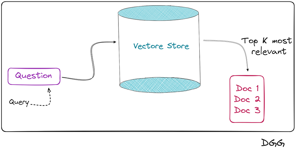
This method is the simplest, in fact its name indicates it. We use this adjective to identify this method for the simple reason that when entering the query into our database, we hope (naively) that it will return the most relevant documents/chunks.
Basically what happens is that we encode the user query with the same transformer with which we created the vector store. Once its vector representation is obtained, we calculate the similarity by calculating the cosine, the distance, etc.
And we collect the top K documents closest/similar to the query.
The flow of this type of retriever can be seen in the following image:
Simplified representation of a Naive retriever (Image by Author).
Keeping the scheme in mind, let’s see how all this looks in the code. We read the database:
from langchain_community.vectorstores import Chroma from langchain_openai import OpenAIEmbeddings import os from dotenv import load_dotenv
# Maximum marginal relevance retrieval # naive_retriever = db.as_retriever(search_type="mmr")
Actually, we have already created our “Naive Retriever”, but to see how it works, we will create the complete RAG that we remember is composed of the following components:
R (Retrieval): Done
A (Augmented): Not yet
G (Generation): Not yet
Augmented & Generation
from langchain_core.prompts import ChatPromptTemplate from langchain_openai import ChatOpenAI
# Augmented TEMPLATE = """ You are happy assistant. Use the context provided below to answer the question.
If you do not know the answer, or are unsure, say you don't know.
We already have the 3 components of our RAG. All that remains is to assemble them, and for this we will use the langchain chains to create a RAG.
I don’t know if you know the language created by langchain for creating chains in a more efficient way. This language is known as LCEL (LangChain Expression Language). If you are new to this way of creating chains in langchain, I leave you a very good tutorial here:
Finally, we create our RAG using Langchain’s own chain creation language (LCEL):
from langchain_core.runnables import RunnablePassthrough, RunnableParallel from operator import itemgetter from langchain_core.output_parsers import StrOutputParser
naive_retrieval_chain.invoke( "Did people generally like John Wick?")
# response: 'Yes, people generally liked John Wick.'
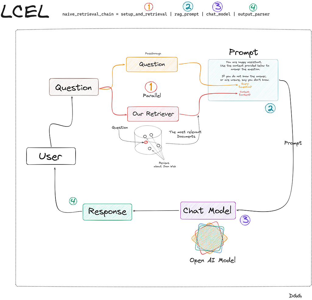
This is the simplest way to create a chain for a RAG. In the Jupyter notebook you can find the same chain but more robust. Since I don’t want us to get lost on this topic now, I have only shown the simplest form. Also so that we understand what is happening in the code above, I have created this very clarifying diagram:
Creation of a RAG with Langchain and its LCEL language (Image by Author).
Great, we’re done creating our Naive RAG. Let’s move on to the next method.
Imagine that we have created a RAG to recognize possible diseases by introducing some of their symptoms in the consultation. In the event that we have a Naive RAG, we may collect a series of possible diseases that only coincide in one or two symptoms, leaving our tool in a bit of a bad place.
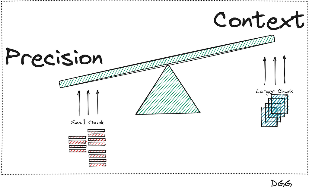
This is an ideal case to use Parent Doc Retriever. And the type of technique consists of cutting large chunks (parent chunk) into even smaller pieces (child chunk). By having small chunks, the information they contain is more concentrated and therefore, its informative value is not diluted between paragraphs of text.
There is a small problem in all this:
If we want to be precise in searching for the most relevant documents, we need to break our documents into small chunks.
But it is also very important to provide good context to the LLM, which is achieved by providing larger chunks.
What has been said can be seen in the following image:
Representation of the balance between these two concepts/metrics (Image by Author).
It seems that there is no way out of the problem, since when we increase the precision, the context is reduced, and vice versa. This is when this method appears that will solve our lives.
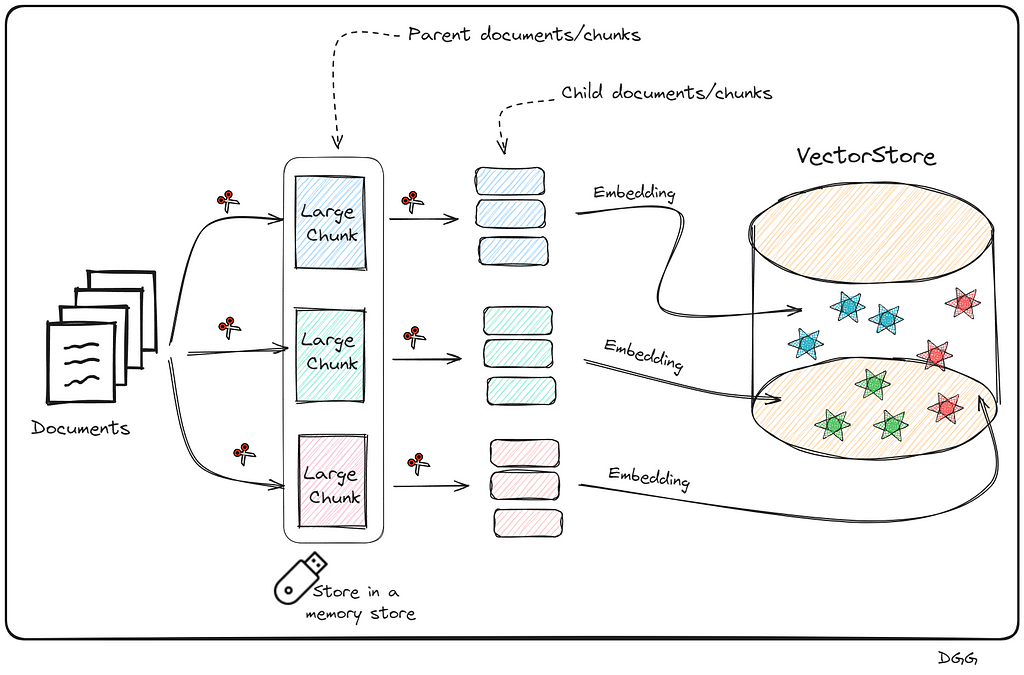
The main idea is to further chop the large chunks (Parent chunks/documents) into smaller chunks (Child Chunks/documents). Once this is done, perform the search for the most relevant top K documents with the child chunks, and return the parents chunks to which the top K child document belongs.
We already have the main idea, now let’s get it down to earth. The best way to explain it is step by step:
Obtain the documents and create the large chunks (Parent chunks)
Perform a split of each of the parent chunks for the growth of the child chunks.
Save the child chunks (Vector Representation) in the Vector Store.
Save the parent chunks in memory (We do not need to create their vector representation).
What has been said can be seen in the following image:
Visual representation of how child chunks are created from parent chunks, and their storage. These are necessary steps to create a parent document retriever (Image by Author).
This may seem very complex to create, since we have to create a new database with the small chunks, save the parent chunks in memory. Additionally, know which parent chunk each child chunk belongs to. Thank goodness Langchain exists and the way to build it is super simple.
Surely you have come to the conclusion that it is necessary to create a new vector store for this method. Furthermore, in the case of reviews of the John Wick movies, such as the data source with CSV files, it is not necessary to perform the first split (parent chunks). This is because we can consider each row of our csv files to be a chunk in itself.
Overall, let’s visualize the following image that reflects how this method works:
Visual representation of how a Parent Document Retriever works (Image by Author).
Going to code it is represented as follows:
from langchain.retrievers import ParentDocumentRetriever from langchain.storage import InMemoryStore from langchain_text_splitters import RecursiveCharacterTextSplitter from langchain_openai import OpenAIEmbeddings from langchain_community.vectorstores import Chroma
# documents = Read csv files. Check jupyter notebook for more details
parent_docs = documents
# Embedding Model embeddings = OpenAIEmbeddings(model="text-embedding-3-small")
# Splitters child_splitter = RecursiveCharacterTextSplitter(chunk_size=200) # We don't need a parent splitter because the data cames from CSV file, and each row is a parent doc. # parent_splitter = RecursiveCharacterTextSplitter(chunk_size=800)
# Stores store = InMemoryStore() vectorstore = Chroma(embedding_function=embeddings, collection_name="fullDoc", persist_directory="./JohnWick_db_parentsRD")
Something intuitive about what happens here is that the number of chunks in the vector store (number of child chunks) should be much higher than the number of documents stored in memory (parent chunks). With the following code we can check it:
print(f"Number of parent chunks  is: {len(list(store.yield_keys()))}")

print(f"Number of child chunks is: {len(parent_document_retriever.vectorstore.get()['ids'])}")

'''
Number of parent chunks  is: 75
Number of child chunks is: 3701
'''
Great, we would already have our Parent Document Retriever, we just need to create our RAG based on this retriever and that would be it. It would be done exactly the same as in the previous method. I attach the code for creating the chain in langchain. To see more details, take a look at the jupyter notebook.
Note that it is exactly the same as in the previous case, only with the small difference that in the “setup_and_retrieval” variable, we configure that we want to use our “parent_document_retriever”, instead of the “naive_retriever”.
This is possibly one of the most optimal methods to improve the efficiency of our retriever.
Its main feature is that it is capable of performing searches in the vector store, applying filters based on the metadata.
We know that when we apply a “Naive retrieval”, we are calculating the similarity of all the chunks of the vector database with the query. The more chunks the vector store has, the more similarity calculations will have to be done. Now, imagine being able to do a prior filter based on the metadata, and after selecting the chunks that meet the conditions imposed in relation to the metadata, calculate similarities. This can drastically reduce computational and time cost.
Let’s look at a use case to fully understand when to apply this type of retreival.
Let’s imagine that we have stored in our vector database a large number of experiences and leisure offers (Ex: surf classes, zip line, gastronomic route, etc.). The description of the experience is what we have encoded, using our embedding model. Additionally, each offer has 3 key values or metadata: Date, price and place.
Let’s imagine that a user is looking for an experience of this style: An experience in nature, that is for the whole family and safe. Furthermore, the price must be less than $50 and the place is California.
Something is clear here
WE DO NOT WANT YOU TO RETURN US ACTIVITY/EXPERIENCES THAT DO NOT MEET THE PRICE OR PLACE THAT THE USER REQUESTS.
Therefore, it does not make sense to calculate similarities with chunks/experiences that do not comply with the metadata filter.
This case is ideal for applying Self Query Retriever. What this type of retriever allows us is to perform a first filter through the metadata, and then perform the similarity calculation between the chunks that meet the metadata requirements and the user input.
This technique can be summarized in two very specific steps:
Query Constructor
Query Translater
Query Constructor
The objective of the step called “Query Constructor” is to create the appropriate query and filters according to the user input.
Who is in charge of applying the corresponding filters and how do you know what they are?
For this we are going to use an LLM. This LLM will have to be able to decide which filters to apply and when. We will also have to explain beforehand what the metadata is and what each of them means. In short, the prompt must contain 3 key points:
Context: Personality, how you should act, output format, etc.
Metadata: Information about available metadata.
Query: The user’s query/input/question.
The output generated by the LLM cannot be directly entered into the database. Therefore, the so-called “Query Translater” is needed.
Query Translater
This is a module in charge of translating the output of the LLM (Query Constructor) into the appropriate format to perform the query. Depending on the vector database you use, you will have to use one or the other. In my case I used Chroma db, therefore, I need a translator focused on this database. Luckily, Langchain has specific database translators for almost all of them.
As you may have already noticed, I am a big fan of diagrams. Let’s look at the following which provides quite a bit of clarity to the matter:
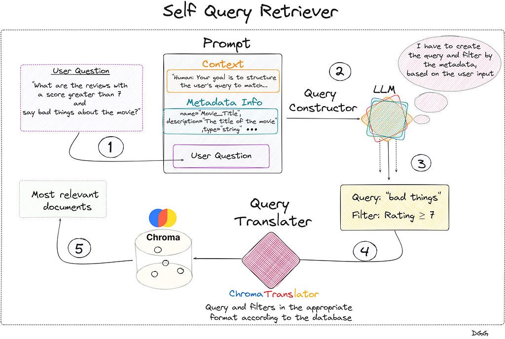
Visual representation of how a Self Query Retriever works (Image by Author).
Regarding the previous image, we see that everything begins with the user’s query. We create the prompt that contains the 3 key fields and is introduced to the LLM that generates a response with two key fields: “Query” and “Filter”. This is fed into the query translator which translates these two fields into the correct format needed by Chroma DB. Performs the query and returns the most relevant documents based on the user’s initial question.
Something to emphasize is that the query entered by the user does not have to be the same as the one entered into the database. In the diagram shown, it can be seen that the LLM, taking into account the available metadata and the user’s question, detects that it can create a filter with the “Rating” metadata. It also creates a new query based on the user’s query.
Let’s look at all this in code. As I have explained, it is very important to provide the LLM with a detailed description of the metadata available in the vector store. This translates into the following piece of code:
from langchain.chains.query_constructor.base import AttributeInfo
from langchain.retrievers.self_query.base import SelfQueryRetriever
from langchain_openai import ChatOpenAI
from langchain.retrievers.self_query.chroma import ChromaTranslator


metadata_field_info = [
    AttributeInfo(
        name="Movie_Title",
        description="The title of the movie",
        type="string",
    ),
    AttributeInfo(
        name="Review_Date",
        description="The date of the review",
        type="string",
    ),
    AttributeInfo(
        name="Review_Title",
        description="The title of the review",
        type="string",
    ),
    AttributeInfo(
        name="Review_Url",
        description="The URL of the review",
        type="string",
    ),
    AttributeInfo(
        name="Author",
        description="The author of the review",
        type="string",
    ),
    AttributeInfo(
        name="Rating",
        description="A 1 to 10 rating for the movie",
        type="integer",
    )
]
To define our retrieval we must define the following points:
The LLM to use
The embedding model to be used
The vector basis that is accessed
A description of what information can be found in the documents of this vector base.
The metadata description
The Query translator you want to use
Let’s see what it looks like in code:
document_content_desription = "A review of the Jonh Wick movie." embeddings = OpenAIEmbeddings(model="text-embedding-3-small") chat_model = ChatOpenAI()
Let’s see with a very clear example how we have greatly improved our RAG by using this type of retriever. First we use a naive retriever and then a self query retriever.
Question = "Make a summary of the reviews that talk about John Wick 3 and have a score higher than 7" response = naive_retrieval_chain.invoke(Question) print(response)
''' I don't know the answer. ''' ------------------------------------------------------------------------
Context Windows: The more documents we obtain from the vectore store, the more information the LLM will have to give a good answer.
Recall: The more documents are retrieved from the vector store, the probability of obtaining irrelevant chunks is greater and therefore, the recall decreases (Not a good thing).
There seems to be no solution for this problem. When we increase one of the metrics, the other seems destined to decrease. Are we sure about that?
This is when this technique, compression retriever, is presented, focusing on the reranking technique. Let’s say that this technique consists of two very different steps:
Step 1: Get a good amount of relevant docs based on the input/question. Normally we set the most relevant K.
Step 2: Recalculate which of these documents are really relevant. discarding the other documents that are not really useful (Compression).
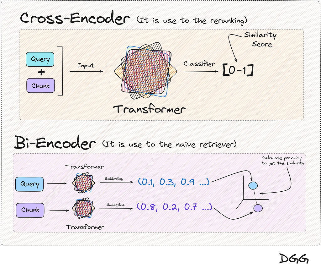
For the first step, what is known as Bi-Encoder is used, which is nothing more than what we usually use to make a basic RAG. Vectorize our documents. vectorize the query and calculate the similarity with any metric of our choice.
The second step is something different from what we are used to seeing. This recalculation/reranking is executed by the reranking model or cross-encoder.
These models expect two documents/texts as input, returning a similarity score between the pair.
If one of these two inputs is the query and the other is a chunk, we can calculate the similarity between the two.
These two methods can be displayed as follows:
Visual representation of the two methods presented in the post to calculate the similarity between texts (Image by Author).
You will have realized that the two methods in the end provide the same result, a metric that reflects the similarity between two texts. And this is totally true, but there is a key feature:
The result returned by the cross encoder is much more reliable than with the Bi-encoder
Okay, it works better, then, because we don’t use it directly with all chunks, instead of just the top K chunks. Because it would be terribly expensive in time and money/computation. For this reason, we make a first filter of the chunks closest in similarity to the query,reducing the use of the reranking model to only K times.
A good question would be where to find the Cross-Encoder models? We are lucky that there are open source models that we can find in HuggingFace, but for the practical case of this post we are going to use the model made available by the company Cohere.
To better understand the architecture of this method, let’s look at a visual example.
Visual representation of how a Contextual Compression Retriever (Reranking) works (Image by Author).
The image shows the steps:
1º) We obtain the query, which we encode in its vector form with a transformer and we introduce it into the vector base.
2º) Collect the documents most similar to the query from our database. We can use any retriever method.
3º) Next we use the Cohere cross-encoder model. In the example in the image, this model will be used a total of 4 times. Remember that the input of this model will be the query and a document/chunk, to collect the similarity of these two texts.
4º) The 4 calls have been made to this model in the previous step and 4 new values (between 0 and 1) of the similarity between the query and each of the documents have been obtained. As can be seen, the chunk number 1 obtained in the previous steps, after the reranking, is now in 4th place.
5º) We add the first 3 chunks most relevant to the context.
Returning again to the computational cost and time, if the cross-encoders were applied directly, think that with each new query, the similarity of the query with each of the documents should be calculated. Something that is not optimal at all.
On the other hand, using Bi-Encoders, the vector representation of the documents is the same for each new query.
We then have a much superior method that is expensive to execute, and on the other hand, another method that works well but does not have a large computational cost with each new query. All this ends with the conclusion of unifying these two methods for a better RAG. And this is known as the Contextual Compression with reranking method.
Let’s move on to the code part. Let’s remember that this method uses a retreiver, which in our case will be a Naive Retriever:
As simple as that. Let’s see a comparison between a Naive Retriever and a Reranking Retriever:
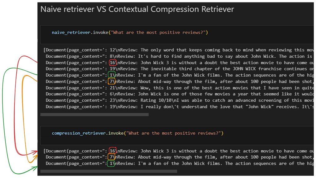
Example of how the reranking method recalculates the similarity between the query and the chunks. This causes the most relevant documents returned by the first retriever (In our case, Naive retriever), to be completely reordered. The 3 best are collected as shown (Image by Author).
As we see, Naive returns us the top 10 chunks/documents. After performing the reranking and obtaining the 3 most relevant documents/chunks, there are noticeable changes. Notice how document number 16, which is in third position in relation to its relevance in the first retriever, becomes first position when performing the reranking.
Conclusion
We have seen that depending on the characteristics of the case where we want to apply a RAG, we will want to use one method or another. Furthermore, there may be the case in which one does not know which retriever method to use. For this, there are different libraries to evaluate your rags.
There are several tools for this purpose. Some of those options that I personally recommend are the combination of RAGAS and LangSmith.
Dive into AlexNet, the first modern CNN, understand its mathematics, implement it from scratch, and explore its applications.
Image generated by DALL-E
Convolutional Neural Networks (CNNs) are a specialized kind of deep neural networks designed primarily for processing structured array data such as images. CNNs operate by recognizing patterns directly from pixel data of images, eliminating the need for manual feature extraction. They are particularly powerful in understanding the spatial hierarchy in images, utilizing learnable filters that process data in patches and thus preserving the spatial relationships between pixels.
These networks are incredibly effective at tasks that involve large amounts of visual data and are widely used in applications ranging from image and video recognition to real-time object detection, playing pivotal roles in advancements like facial recognition technology and autonomous vehicles.
In this article, we’ll explore AlexNet, a groundbreaking CNN architecture that has significantly influenced the field of computer vision. Known for its robust performance on various visual recognition tasks, AlexNet utilizes deep learning to interpret complex imagery directly. We’ll break down the mathematics behind its operations and the coding framework that powers it.
AlexNet is a pioneering deep learning network that rose to prominence after winning the ImageNet Large Scale Visual Recognition Challenge in 2012. Developed by Alex Krizhevsky, Ilya Sutskever, and Geoffrey Hinton, AlexNet significantly lowered the top-5 error rate to 15.3% from the previous best of 26.2%, setting a new benchmark for the field. This achievement highlighted the effectiveness of CNNs that use ReLU activations, GPU acceleration, and dropout regularization to manage complex image classification tasks across large datasets.
The model comprises several layers that have become standard in most deep-learning CNNs today. These include convolutional layers, max-pooling, dropout, fully connected layers, and a softmax output layer. The model’s success demonstrated the practicality of deeper network architectures through creative approaches to design and training.
In this article, we will break down the sophisticated design and mathematical principles that underpin AlexNet. We’ll also review AlexNet’s training procedures and optimization techniques, and we will build it from scratch using PyTorch.
2: Overview of AlexNet Architecture
AlexNet Architecture — Image by Author
2.1: General Layer Structure
AlexNet’s architecture cleverly extracts features through a hierarchical layering system where each layer builds on the previous layers’ outputs to refine the feature extraction process. Here’s a detailed breakdown of its layers and functions:
Input Image The model processes input images resized to 227×227 pixels. Each image has three channels (Red, Green, and Blue), reflecting standard RGB encoding.
Layer Configuration It consists of eight primary layers that learn weights, five of which are convolutional, and the remaining three are fully connected. Between these layers, activation functions, normalization, pooling, and dropout are strategically applied to improve learning efficacy and combat overfitting.
Convolutional Layers The initial layer uses 96 kernels (filters) sized 11x11x3, which convolve with the input image using a stride of 4 pixels. This large stride size helps reduce the output spatial volume size significantly, making the network computationally efficient right from the first layer.
Outputs from the first layer undergo normalization and max-pooling before reaching the second convolutional layer, which consists of 256 kernels each of size 5x5x48. The use of 48 feature maps each corresponds to separate filtered outputs from the previous layer, allowing this layer to mix features effectively.
The third convolutional layer does not follow with pooling or normalization, which typically helps to maintain the feature map’s richness derived from previous layers. It includes 384 kernels of size 3x3x256, directly connected to the outputs of the second layer, enhancing the network’s ability to capture complex features.
The fourth convolutional layer mirrors the third layer’s configuration but uses 384 kernels of size 3x3x192, enhancing the depth of the network without altering the layer’s spatial dimensions.
The final convolutional layer employs 256 kernels of size 3x3x192 and is followed by a max-pooling layer, which helps to reduce dimensionality and provides rotational and positional invariance to the features being learned.
Fully Connected Layers The first fully connected layer is a dense layer with 4096 neurons. It takes the flattened output from the preceding convolutional layers (transformed into a 1D vector) and projects it onto a high-dimensional space to learn non-linear combinations of the features.
The second fully connected layer also features 4096 neurons and includes dropout regularization. Dropout helps prevent overfitting by randomly setting a fraction of input units to zero during training, which encourages the network to learn more robust features that are not reliant on any small set of neurons.
The final fully connected layer comprises 1000 neurons, each corresponding to a class of the ImageNet challenge. This layer is essential for class prediction, and it typically utilizes a softmax function to derive the classification probabilities.
2.2: Output Layer and Softmax Classification
The final layer in AlexNet is a softmax regression layer which outputs a distribution over the 1000 class labels by applying the softmax function to the logits of the third fully connected layer.
The softmax function is given by:
Softmax Function — Image by Author
where zi are the logits or the raw prediction scores for each class from the final fully connected layer.
This layer essentially converts the scores into probabilities by comparing the exponentiated score of each class with the sum of exponentiated scores for all classes, highlighting the most probable class.
The softmax layer not only outputs these probabilities but also forms the basis for the cross-entropy loss during training, which measures the difference between the predicted probability distribution and the actual distribution (the true labels).
3: In-depth Analysis of AlexNet Components
3.1: ReLU Nonlinearity
The Rectified Linear Unit (ReLU) has become a standard activation function for deep neural networks, especially CNNs like AlexNet. Its simplicity allows models to train faster and converge more effectively compared to networks using sigmoid or tanh functions.
The mathematical representation of ReLU is straightforward:
ReLU Function — Image by Author
This function outputs x if x is positive; otherwise, it outputs zero.
ReLU Plot — Image by Author
Graphically, it looks like a ramp function that increases linearly for all positive inputs and is zero for negative inputs.
Advantages Of Sigmoid Over Tanh ReLU has several advantages over traditional activation functions such as sigmoid:
Sigmoid Function — Image by Author
and hyperbolic tangent:
Tanh Function — Image by Author
ReLU helps neural networks converge faster by addressing the vanishing gradient problem. This problem occurs with sigmoid and tanh functions where gradients become very small (approach zero) as inputs become large, in either positive or negative direction. This small gradient slows down the training significantly as it provides very little update to the weights during backpropagation. In contrast, the gradient of the ReLU function is either 0 (for negative inputs) or 1 (for positive inputs), which simplifies and speeds up gradient descent.
It promotes sparsity of the activation. Since it outputs zero for half of its input domain, it inherently produces sparse data representations. Sparse representations seem to be more beneficial than dense representations (as typically produced by sigmoid or tanh functions), particularly in large-scale image recognition tasks where the inherent data dimensionality is very high but the informative part is relatively low.
Moreover, ReLU involves simpler mathematical operations. For any input value, this activation function requires a single max operation, whereas sigmoid and tanh involve more complex exponential functions, which are computationally more expensive. This simplicity of ReLU leads to much faster computational performance, especially beneficial when training deep neural networks on large datasets.
Because the negative part of ReLU’s function is zeroed out, it avoids the problem of outputs that do not change in a non-linear fashion as seen with sigmoid or tanh functions. This characteristic allows the network to model the data more cleanly and avoid potential pitfalls in training dynamics.
AlexNet was one of the pioneering convolutional neural networks to leverage parallel GPU training, managing its deep and computation-heavy architecture. The network operates on two GPUs simultaneously, a core part of its design that greatly improves its performance and practicality.
Layer-wise Distribution AlexNet’s layers are distributed between two GPUs. Each GPU processes half of the neuron activations (kernels) in the convolutional layers. Specifically, the kernels in the third layer receive inputs from all kernel maps of the second layer, whereas the fourth and fifth layers only receive inputs from kernel maps located on the same GPU.
Communication Across GPUs The GPUs need to communicate at specific layers crucial for combining their outputs for further processing. This inter-GPU communication is essential for integrating the results of parallel computations.
Selective Connectivity Not every layer in AlexNet is connected across both GPUs. This selective connectivity reduces the amount of data transferred between GPUs, cutting down on communication overhead and enhancing computation efficiency.
This strategy of dividing not just the dataset but also the network model across two GPUs enables AlexNet to handle more parameters and larger input sizes than if it were running on a single GPU. The extra processing power allows AlexNet to handle its 60 million parameters and the extensive computations required for training deep networks on large-scale image classification tasks efficiently.
Training with larger batch sizes is more feasible with multiple GPUs. Larger batches provide more stable gradient estimates during training, which is vital for efficiently training deep networks. While not directly a result of using multiple GPUs, the ability to train with larger batch sizes and more rapid iteration times helps combat overfitting. The network experiences a more diverse set of data in a shorter amount of time, which enhances its ability to generalize from the training data to unseen data.
3.3: Local Response Normalization
Local Response Normalization (LRN) in AlexNet is a normalization strategy that plays a crucial role in the network’s ability to perform well in image classification tasks. This technique is applied to the output of the ReLU non-linearity activation function.
LRN aims to encourage lateral inhibition, a biological process where activated neurons suppress the activity of neighboring neurons in the same layer. This mechanism works under the “winner-takes-all” principle, where neurons showing relatively high activity suppress the less active neurons around them. This dynamic allows the most significant features relative to their local neighborhood to be enhanced while suppressing the lesser ones.
The LRN layer computes a normalized output for each neuron by performing a sort of lateral inhibition by damping the responses of neurons when their locally adjacent neurons exhibit high activity.
Given a neuron’s activity ax, yi at position (x, y) in the feature map i, the response-normalized activity bx, yi is given by:
Local Response Normalization Formula — Image by Author
where:
ax, yi is the activity of a neuron computed by applying kernel i at position (x, y) and then applying the ReLU function.
N is the total number of kernels in the layer.
The sum runs over n neighboring kernel maps at the same spatial position, and N is the total number of kernels.
k, α, β are hyperparameters whose values are predetermined (in AlexNet, typically n=5, k=2, α=10e−4, β=0.75).
bx, yi is the normalized response of the neuron.
Local Response Normalization (LRN) serves to implement a form of local inhibition among adjacent neurons, which is inspired by the concept of lateral inhibition found in biological neurons. This inhibition plays a vital role in several key areas:
Activity Regulation LRN prevents any single feature map from overwhelming the response of the network by penalizing larger activations that lack support from their surroundings. This squaring and summing of neighboring activations ensures no single feature disproportionately influences the output, enhancing the model’s ability to generalize across various inputs.
Contrast Normalization By emphasizing patterns that stand out relative to their neighbors, LRN functions similarly to contrast normalization in visual processing. This feature highlights critical local features in an image more effectively, aiding in the visual differentiation process.
Error Rate Reduction Incorporating LRN in AlexNet has helped reduce the top-1 and top-5 error rates in the ImageNet classification tasks. It manages the high activity levels of neurons, thereby improving the overall robustness of the network.
3.4: Overlapping Pooling
Overlapping pooling is a technique used in convolutional neural networks (CNNs) to reduce the spatial dimensions of the input data, simplify the computations, and help control overfitting. It modifies the standard non-overlapping (traditional) max-pooling by allowing the pooling windows to overlap.
Traditional Max Pooling In traditional max pooling, the input image or feature map is divided into distinct, non-overlapping regions, each corresponding to the size of the pooling filter, often 2×2. For each of these regions, the maximum pixel value is determined and output to the next layer. This process reduces the data dimensions by selecting the most prominent features from non-overlapping neighborhoods.
For example, assuming a pooling size (z) of 2×2 and a stride (s) of 2 pixels, the filter moves 2 pixels across and 2 pixels down the input field. The stride of 2 ensures there is no overlap between the regions processed by the filter.
Overlapping Pooling in AlexNet Overlapping pooling, used by AlexNet, involves setting the stride smaller than the pool size. This approach allows the pooling regions to overlap, meaning the same pixel may be included in multiple pooling operations. It increases the density of the feature mapping and helps retain more information through the layers.
For example, using a pooling size of 3×3 and a stride of 2 pixels. This configuration means that while the pooling filter is larger (3×3), it moves by only 2 pixels each time it slides over the image or feature map. As a result, adjacent pooling regions share a column or row of pixels that gets processed multiple times, enhancing feature integration.
3.5: Fully Connected Layers and Dropout
In the architecture of AlexNet, after several stages of convolutional and pooling layers, the high-level reasoning in the network is done by fully connected layers. Fully connected layers play a crucial role in transitioning from the extraction of feature maps in the convolutional layers to the final classification.
A fully connected (FC) layer takes all neurons in the previous layer (whether they are the output of another fully connected layer, or a flattened output from a pooling or convolutional layer) and connects each of these neurons to every neuron it contains. In AlexNet, there are three fully connected layers following the convolutional and pooling layers.
The first two fully connected layers in AlexNet have 4096 neurons each. These layers are instrumental in integrating the localized, filtered features that the prior layers have identified into global, high-level patterns that can represent complex dependencies in the inputs. The final fully connected layer effectively acts as a classifier: with one neuron for each class label (1000 for ImageNet), it outputs the network’s prediction for the input image’s category.
Each neuron in these layers applies a ReLU (Rectified Linear Unit) activation function except for the output layer, which uses a softmax function to map the output logits (the raw prediction scores for each class) to a probabilistic distribution over the classes.
The output from the final pooling or convolutional layer typically undergoes flattening before being fed into the fully connected layers. This process transforms the 2D feature maps into 1D feature vectors, making them suitable for processing via traditional neural network techniques. The final layer’s softmax function then classifies the input image by assigning probabilities to each class label based on the feature combinations learned through the network.
3.6: Dropout
Dropout is a regularization technique used to prevent overfitting in neural networks, particularly effective in large networks like AlexNet. Overfitting occurs when a model learns patterns specific to the training data, but which do not generalize to new data.
In AlexNet, dropout is applied to the outputs of the first two fully connected layers. Each neuron in these layers has a probability p (commonly set to 0.5, i.e., 50%) of being “dropped,” meaning it is temporarily removed from the network along with all its incoming and outgoing connections.
If you want to dive deep into Dropout’s math and code, I highly recommend you take a look at section 3.4 of my previous article:
In AlexNet, Stochastic Gradient Descent (SGD) is employed to optimize the network during training. This method updates the network’s weights based on the error gradient of the loss function, where the effective tuning of parameters such as batch size, momentum, and weight decay is critical for the model’s performance and convergence. In today’s article, we will use a Pytorch implementation of SGD, and we will cover a high-level view of this popular optimization technique. If you are interested in a low-level view, scraping its math, and building the optimizer from scratch, take a look at this article:
Let’s cover now the main components of SGD and the settings used in AlexNet:
Batch Size The batch size, which is the number of training examples used to calculate the loss function’s gradient for one update of the model’s weights, is set to 128 in AlexNet. This size strikes a balance between computational efficiency — since larger batches require more memory and computation — and the accuracy of error estimates, which benefit from averaging across more examples.
The choice of a batch size of 128 helps stabilize the gradient estimates, making the updates smoother and more reliable. While larger batches provide a clearer signal for each update by reducing noise in the gradient calculations, they also require more computational resources and may sometimes generalize less effectively from training data to new situations.
Momentum Momentum in SGD helps accelerate the updates in the correct direction and smoothens the path taken by the optimizer. It modifies the update rule by incorporating a fraction of the previous update vector. In AlexNet, the momentum value is 0.9, implying that 90% of the previous update vector contributes to the current update. This high level of momentum speeds up convergence towards the loss function’s minimum, which is particularly useful when dealing with small but consistent gradients.
Using momentum ensures that updates not only move in the right direction but also build up speed along surfaces of the loss function’s topology that have consistent gradients. This aspect is crucial for escaping from any potential shallow local minima or saddle points more effectively.
Weight Decay Weight decay acts as a regularization term that penalizes large weights by adding a portion of the weight values to the loss function. AlexNet sets this parameter at 0.0005 to keep the weights from becoming too large, which could lead to overfitting given the network’s large number of parameters.
Weight decay is essential in complex models like AlexNet, which are prone to overfitting due to their high capacity. By penalizing the magnitude of the weights, weight decay ensures that the model does not rely too heavily on a small number of high-weight features, promoting a more generalized model.
The update rule for AlexNet’s weights can be described as follows:
AlexNet Update Formula — Image by Author
Here:
vt is the momentum-enhanced update vector from the previous step.
μ (0.9 for AlexNet) is the momentum factor, enhancing the influence of the previous update.
ϵ is the learning rate, determining the size of the update steps.
∇L represents the gradient of the loss function for the weights.
λ (0.0005 for AlexNet) is the weight decay factor, mitigating the risk of overfitting by penalizing large weights.
w denotes the weights themselves.
These settings help ensure that the network not only learns efficiently but also achieves robust performance on both seen and unseen data, optimizing the speed and accuracy of training while maintaining the ability to generalize well.
4.2: Initialization
Proper initialization of weights and biases and the careful adjustment of the learning rate are critical to training deep neural networks. These factors influence the rate at which the network converges and its overall performance on both training and validation datasets.
Weights Initialization
In AlexNet, the weights for the convolutional layers are initialized from a zero-mean Gaussian distribution with a standard deviation of 0.01. This narrow standard deviation prevents any single neuron from initially overwhelming the output, ensuring a uniform scale of weight initialization.
Similarly, weights in the fully connected layers are initialized from a Gaussian distribution. Special attention is given to the variance of this distribution to keep the output variance consistent across layers, which is crucial for maintaining the stability of deeper networks.
To get a better understanding of this process let’s build the initialization for AlexNet from scratch in Python:
import numpy as np
def initialize_weights(layer_shapes): weights = [] for shape in layer_shapes: if len(shape) == 4: # This is a conv layer: (out_channels, in_channels, filter_height, filter_width) std_dev = 0.01 # Standard deviation for conv layers fan_in = np.prod(shape[1:]) # product of in_channels, filter_height, filter_width elif len(shape) == 2: # This is a fully connected layer: (out_features, in_features) # He initialization: std_dev = sqrt(2. / fan_in) fan_in = shape[1] # number of input features std_dev = np.sqrt(2. / fan_in) # Recommended to maintain variance for ReLU else: raise ValueError("Invalid layer shape: must be 4D (conv) or 2D (fc)")
initialized_weights = initialize_weights(layer_shapes) for idx, weight in enumerate(initialized_weights): print(f"Layer {idx+1} weights shape: {weight.shape} mean: {np.mean(weight):.5f} std dev: {np.std(weight):.5f}")
The initialize_weights function takes a list of tuples describing the dimensions of each layer’s weights. Convolutional layers expect four dimensions (number of filters, input channels, filter height, filter width), while fully connected layers expect two dimensions (output features, input features).
In the convolutional layers standard deviation is fixed at 0.01, aligned with the original AlexNet configuration to prevent overwhelming outputs by any single neuron.
Fully connected layers use He initialization (good practice for layers using ReLU activation) where the standard deviation is adjusted to sqrt(2/fan_in) to keep the output variance consistent, promoting stable learning in deep networks.
For each layer defined in layer_shapes, weights are initialized from a Gaussian (normal) distribution centered at zero with a calculated
Biases Initialization Biases in some convolutional layers are set to 1, particularly in layers followed by ReLU activations. This initialization pushes the neuron outputs into the positive range of the ReLU function, ensuring they are active from the beginning of training. Biases in other layers are initialized at 0 to start from a neutral output.
Like in certain convolutional layers, biases in fully connected layers are also set to 1. This strategy helps to prevent dead neurons at the start of training by ensuring that neurons are initially in the positive phase of activation.
4.3: Strategy for Adjusting the Learning Rate
AlexNet begins with an initial learning rate of 0.01. This rate is high enough to allow significant updates to the weights, facilitating rapid initial progress without being so high as to risk the divergence of the learning process.
The learning rate is decreased by a factor of 10 at predetermined points during the training. This approach is known as “step decay.” In AlexNet, these adjustments typically occur when the validation error rate stops decreasing significantly. Reducing the learning rate at these points helps refine the weight adjustments, promoting better convergence.
Starting with a higher learning rate helps the model overcome potential local minima more effectively. As the network begins to stabilize, reducing the learning rate helps it settle into broad, flat minima that are generally better for generalization to new data.
As training progresses, lowering the learning rate allows for finer weight adjustments. This gradual refinement helps the model to not only fit the training data better but also improves its performance on validation data, ensuring the model is not just memorizing the training examples but genuinely learning to generalize from them.
5: Building AlexNet in Python
In this section, we detail the step-by-step process to recreate AlexNet in Python using PyTorch, providing insights into the class architecture, its initial setup, training procedures, and evaluation techniques.
I suggest you keep this Jupyter Notebook open and accessible, as it contains all the code we will be covering today:
# PyTorch for creating and training the neural network import torch import torch.nn as nn import torch.optim as optim from torch.utils.data.dataset import random_split
# platform for getting the operating system import platform
# torchvision for loading and transforming the dataset import torchvision import torchvision.transforms as transforms
# ReduceLROnPlateau for adjusting the learning rate from torch.optim.lr_scheduler import ReduceLROnPlateau
# numpy for numerical operations import numpy as np
# matplotlib for plotting import matplotlib.pyplot as plt
def forward(self, x): x = self.features(x) x = self.avgpool(x) x = torch.flatten(x, 1) x = self.classifier(x) return x
Initializationclass AlexNet(nn.Module)
class AlexNet(nn.Module):
    def __init__(self, num_classes=1000):
        super(AlexNet, self).__init__()
The AlexNet class inherits from nn.Module, a base class for all neural network modules in PyTorch. Any new network architecture in PyTorch is created by subclassing nn.Module.
The initialization method defines how the AlexNet object should be constructed when instantiated. It optionally takes a parameter num_classes to allow for flexibility in the number of output classes, defaulting to 1000, which is typical for ImageNet tasks.
Here is where the convolutional layers of AlexNet are defined. The nn.Sequential container wraps a sequence of layers, and data passes through these layers in the order they are added.
The first layer is a 2D convolutional layer (nn.Conv2d) with 3 input channels (RGB image), and 64 output channels (feature maps), with a kernel size of 11×11, a stride of 4, and padding of 2 on each side. This layer processes the input image and begins the feature extraction.
nn.ReLU(inplace=True)
Then, we pass the ReLU activation function which introduces non-linearity, allowing the model to learn complex patterns. The inplace=True parameter helps to save memory by modifying the input directly.
nn.MaxPool2d(kernel_size=3, stride=2)
The max-pooling layer reduces the spatial dimensions of the input feature maps, making the model more robust to the position of features in the input images. It uses a window of size 3×3 and a stride of 2.
Additional nn.Conv2d and nn.MaxPool2d layers follow, which further refine and compact the feature representation. Each convolutional layer typically increases the number of feature maps while reducing their dimensionality through pooling, a pattern that helps in abstracting from the spatial input to features that progressively encapsulate more semantic information.
Adaptive Pooling and Classifier
self.avgpool = nn.AdaptiveAvgPool2d((6, 6))
self.avgpool adaptively pools the feature maps to a fixed size of 6×6, which is necessary for matching the input size requirement of the fully connected layers, allowing the network to handle various input dimensions.
Here, we define another sequential container named classifier, which contains the fully connected layers of the network. These layers are responsible for making the final classification based on the abstract features extracted by the convolutional layers.
nn.Dropout() randomly zeroes some of the elements of the input tensor with a probability of 0.5 for each forward call, which helps prevent overfitting.
nn.Linear(256 * 6 * 6, 4096) reshapes the flattened feature maps from the adaptive pooling layer into a vector of size 4096. It connects every input to every output with learned weights.
Finally, nn.ReLU and nn.Dropout calls further refine the learning pathway, providing non-linear activation points and regularization respectively. The final nn.Linear layer reduces the dimension from 4096 to num_classes, outputting the raw scores for each class.
Forward Method
def forward(self, x):
        x = self.features(x)
        x = self.avgpool(x)
        x = torch.flatten(x, 1)
        x = self.classifier(x)
        return x
The forward method dictates the execution of the forward pass of the network:
x = self.features(x) processes the input through the convolutional layers for initial feature extraction.
x = self.avgpool(x) applies adaptive pooling to the features to standardize their size.
x = torch.flatten(x, 1) flattens the output to a vector, preparing it for classification.
x = self.classifier(x) runs the flattened vector through the classifier to generate predictions for each class.
5.2: Early Stopping Class
The EarlyStopping class is used during the training of machine learning models to halt the training process when the validation loss ceases to improve. This approach is instrumental in preventing overfitting and conserving computational resources by stopping the training at the optimal time.
class EarlyStopping:
    """
    Early stopping to stop the training when the loss does not improve after

    Args:
    -----
        patience (int): Number of epochs to wait before stopping the training.
        verbose (bool): If True, prints a message for each epoch where the loss
                        does not improve.
        delta (float): Minimum change in the monitored quantity to qualify as an improvement.
    """
    def __init__(self, patience=7, verbose=False, delta=0):
        self.patience = patience
        self.verbose = verbose
        self.counter = 0
        self.best_score = None
        self.early_stop = False
        self.delta = delta

    def __call__(self, val_loss):
        """
        Args:
        -----
            val_loss (float): The validation loss to check if the model performance improved.

        Returns:
        --------
            bool: True if the loss did not improve, False if it improved.
        """
        score = -val_loss

        if self.best_score is None:
            self.best_score = score
        elif score < self.best_score + self.delta:
            self.counter += 1
            if self.counter >= self.patience:
                self.early_stop = True
        else:
            self.best_score = score
            self.counter = 0
The EarlyStopping class is initialized with several parameters that configure its operation:
patience determines the number of epochs to wait for an improvement in the validation loss before stopping the training. It is set by default to 7, allowing some leeway for the model to overcome potential plateaus in the loss landscape.
verbose controls the output of the class; if set to True, it will print a message for each epoch where the loss does not improve, providing clear feedback during training.
delta sets the threshold for what constitutes an improvement in the loss, aiding in fine-tuning the sensitivity of the early stopping mechanism.
Callable Method
def __call__(self, val_loss):
    score = -val_loss

    if self.best_score is None:
        self.best_score = score
    elif score < self.best_score + self.delta:
        self.counter += 1
        if self.counter >= self.patience:
            self.early_stop = True
    else:
        self.best_score = score
        self.counter = 0
The __call__ method allows the EarlyStopping instance to be used as a function, which simplifies its integration into a training loop. It assesses whether the model’s performance has improved based on the validation loss from the current epoch.
The method first converts the validation loss into a score that should be maximized; this is done by negating the loss (score = -val_loss), as a lower loss is better. If this is the first evaluation (self.best_score is None), the method sets the current score as the initial best_score.
If the current score is less than self.best_score plus a small delta, indicating no significant improvement, the counter is incremented. This counter tracks how many epochs have passed without improvement. If the counter reaches the patience threshold, it triggers the early_stop flag, indicating that training should be halted.
Conversely, if the current score shows an improvement, the method updates self.best_score with the new score and resets the counter to zero, reflecting the new baseline for future improvements.
This mechanism ensures that the training process is only stopped after a specified number of epochs without meaningful improvement, thereby optimizing the training phase and preventing premature cessation that could lead to underfitting models. By adjusting patience and delta, users can calibrate how sensitive the early stopping is to changes in training performance, allowing them to tailor it to specific scenarios and datasets. This customization is crucial for achieving the best possible model given the computational resources and time available.
5.3: Trainer Class
The Trainer class incorporates the entire training workflow, which includes iterating over epochs, managing the training loop, handling backpropagation, and implementing early stopping protocols to optimize training efficiency and efficacy.
class Trainer: """ Trainer class to train the model.
Args: ----- model (nn.Module): Neural network model. criterion (torch.nn.modules.loss): Loss function. optimizer (torch.optim): Optimizer. device (torch.device): Device to run the model on. patience (int): Number of epochs to wait before stopping the training. """ def __init__(self, model, criterion, optimizer, device, patience=7): self.model = model self.criterion = criterion self.optimizer = optimizer self.device = device self.early_stopping = EarlyStopping(patience=patience) self.scheduler = ReduceLROnPlateau(self.optimizer, 'min', patience=3, verbose=True, factor=0.5, min_lr=1e-6) self.train_losses = [] self.val_losses = [] self.gradient_norms = []
def train(self, train_loader, val_loader, epochs): """ Train the model.
Args: ----- train_loader (torch.utils.data.DataLoader): DataLoader for training dataset. val_loader (torch.utils.data.DataLoader): DataLoader for validation dataset. epochs (int): Number of epochs to train the model. """ for epoch in range(epochs): self.model.train() for images, labels in train_loader: images, labels = images.to(self.device), labels.to(self.device)
self.optimizer.zero_grad() outputs = self.model(images) loss = self.criterion(outputs, labels) loss.backward() self.optimizer.step()
# Log the training and validation loss print(f'Epoch {epoch+1}, Training Loss: {loss.item():.4f}, Validation Loss: {val_loss:.4f}')
if self.early_stopping.early_stop: print("Early stopping") break
def evaluate(self, test_loader): """ Evaluate the model on the test dataset.
Args: ----- test_loader (torch.utils.data.DataLoader): DataLoader for test dataset.
Returns: -------- float: Average loss on the test dataset. """ self.model.eval() total_loss = 0 with torch.no_grad(): for images, labels in test_loader: images, labels = images.to(self.device), labels.to(self.device)
outputs = self.model(images) loss = self.criterion(outputs, labels) total_loss += loss.item()
return total_loss / len(test_loader)
def accuracy(self, test_loader): """ Calculate the accuracy of the model on the test dataset.
Args: ----- test_loader (torch.utils.data.DataLoader): DataLoader for test dataset.
Returns: -------- float: Accuracy of the model on the test dataset. """ self.model.eval() correct = 0 total = 0 with torch.no_grad(): for images, labels in test_loader: images, labels = images.to(self.device), labels.to(self.device)
The Trainer class is initialized with the neural network model, the loss function, the optimizer, and the device (CPU or GPU) on which the model will run. This setup ensures that all model computations are directed to the appropriate hardware.
It also configures early stopping and learning rate reduction strategies:
EarlyStopping: Monitors validation loss and stops training if there hasn’t been an improvement for a given number of epochs (patience).
ReduceLROnPlateau: Reduces the learning rate when the validation loss stops improving, which helps in fine-tuning the model by taking smaller steps in the weight space.
Here, train_losses and val_losses collect the loss per epoch for training and validation phases, respectively, allowing for performance tracking and later analysis. gradient_norms could be used to store the norms of the gradients, useful for debugging and ensuring that gradients are neither vanishing nor exploding.
Training Method
def train(self, train_loader, val_loader, epochs): for epoch in range(epochs): self.model.train() for images, labels in train_loader: images, labels = images.to(self.device), labels.to(self.device)
self.optimizer.zero_grad() outputs = self.model(images) loss = self.criterion(outputs, labels) loss.backward() self.optimizer.step()
# Log the training and validation loss print(f'Epoch {epoch+1}, Training Loss: {loss.item():.4f}, Validation Loss: {val_loss:.4f}')
if self.early_stopping.early_stop: print("Early stopping") break
The train method orchestrates the model training over a specified number of epochs. It processes batches of data, performs backpropagation to update model weights, and evaluates model performance using the validation set at the end of each epoch.
After each epoch, it logs the training and validation losses and updates the learning rate if necessary. The loop may break early if the early stopping condition is triggered, which is checked after evaluating the validation loss.
Evaluation and Accuracy Methods
def evaluate(self, test_loader): self.model.eval() total_loss = 0 with torch.no_grad(): for images, labels in test_loader: images, labels = images.to(self.device), labels.to(self.device)
outputs = self.model(images) loss = self.criterion(outputs, labels) total_loss += loss.item()
return total_loss / len(test_loader)
def accuracy(self, test_loader): self.model.eval() correct = 0 total = 0 with torch.no_grad(): for images, labels in test_loader: images, labels = images.to(self.device), labels.to(self.device)
The evaluate method assesses the model’s performance on a given dataset (typically the validation or test set) and returns the average loss. This method sets the model to evaluation mode, iterates through the dataset, computes the loss for each batch, and calculates the average loss across all batches.
accuracy calculates the accuracy of the model on a given dataset by comparing the predicted labels with the actual labels. This method processes the dataset in evaluation mode, uses the model’s predictions to compute the number of correct predictions, and returns the accuracy percentage.
This method visualizes the training and validation losses, smoothed over a specified window of epochs to highlight trends more clearly, such as reductions in loss over time or potential points where the model began to overfit.
5.4: Data Preprocessing
To effectively train the AlexNet model, proper data preprocessing is necessary to conform to the input requirements of the model, specifically, the dimension and normalization standards that AlexNet was originally designed with.
Transform
transform = transforms.Compose([
    transforms.Resize((224, 224)),  # Resize the images to 224x224 for AlexNet compatibility
    transforms.ToTensor(),  # Convert images to PyTorch tensors
    transforms.Normalize((0.5, 0.5, 0.5), (0.5, 0.5, 0.5))  # Normalize the tensors
])
transforms.Resize((224, 224)) adjusts the size of the images to 224×224 pixels, matching the input size required by the AlexNet model, ensuring that all input images are of the same size.
transforms.ToTensor() converts the images from a PIL format or a NumPy array to a PyTorch tensor, an essential step as PyTorch models expect inputs in tensor format.
transforms.Normalize((0.5, 0.5, 0.5), (0.5, 0.5, 0.5)) normalizes the image tensors; this specific normalization adjusts the mean and standard deviation for all three channels (RGB) to 0.5, effectively scaling pixel values to the range [-1, 1]. This step is crucial as it standardizes the inputs, facilitating the model’s learning process.
Here, we load the CIFAR-10 dataset for both training and testing. You might wonder why we didn’t choose the ImageNet dataset, which is known for its extensive use in training models that compete in the ImageNet challenge. The reason is practical: ImageNet requires significant computational resources and lengthy training times, which I wouldn’t recommend attempting on a standard laptop. Instead, we opt for the CIFAR-10 dataset, which includes 60,000 32×32 color images distributed across 10 different classes, with 6,000 images per class.
Disclaimer: The CIFAR-10 dataset is open source and available for use under the MIT License. This license allows for wide freedom in use, including commercial applications.
The training data is split to set aside 80% for training and 20% for validation. This practice is common to tune the model on unseen data, enhancing its ability to generalize well.
DataLoader objects are created for the training, validation, and test datasets with a batch size of 64. Shuffling is enabled for the training data to ensure randomness, which helps the model learn more effectively by reducing the chance of learning spurious patterns from the order of the data.
imshow(torchvision.utils.make_grid(images[:5])) print(' '.join('%5s' % classes[labels[j]] for j in range(5)))
First, we need to unnormalize the image (img = img / 2 + 0.5). Here imshow converts it from a tensor to a NumPy array, and changes the order of dimensions to fit what matplotlib.pyplot.imshow() expects.
Then, we display the first 5 images in the dataset:
First 5 images in CIFAR-10 dataset — Image by Author
5.5: Model Training and Evaluation
Finally, we set up the training environment for an AlexNet model, executing the training process, and evaluating the model’s performance on a test dataset using PyTorch.
But first, we need to ensure the best computational resource (CPU or GPU) to use, which maximizes performance efficiency.
# Check the system's operating system
if platform.system() == 'Darwin':  # Darwin stands for macOS
    try:
        device = torch.device('cuda')
        _ = torch.zeros(1).to(device)  # This will raise an error if CUDA is not available
    except:
        device = torch.device('mps' if torch.backends.mps.is_built() else 'cpu')
else:
    device = torch.device('cuda' if torch.cuda.is_available() else 'cpu')
Here, we identify whether the system is macOS (‘Darwin’) and tries to configure CUDA for use. If CUDA is unavailable, which is common on macOS without NVIDIA GPUs, it opts for MPS (Apple’s Metal Performance Shaders) if available, or CPU otherwise.
On operating systems other than macOS, it directly attempts to utilize CUDA and defaults to CPU if CUDA isn’t available.
Model, Loss Function, and Optimizer Initialization Next, we initialize the AlexNet model, specifying the computational device, and set up the loss function and optimizer:
An instance of AlexNet is created with 10 classes, and it is immediately transferred to the determined device (GPU or CPU). This ensures all computations for the model are performed on the specified device.
The CrossEntropyLoss function is used for training, which is typical for multi-class classification problems.
The SGD (Stochastic Gradient Descent) optimizer is initialized with the model’s parameters, a learning rate of 0.01, and a momentum of 0.9. These are standard values to start with for many vision-based tasks.
Training the Model The model undergoes training over a specified number of epochs, handling data in batches, calculating loss, performing backpropagation, and applying early stopping based on the validation loss:
The train method trains the model for 50 epochs using the training and validation data loaders. This method meticulously processes batches from the data loaders, computes the loss, performs backpropagation to update weights, and evaluates the model periodically using the validation dataset to implement early stopping if no improvement is observed in the validation loss.
Model Evaluation After training, the model’s performance is assessed on the test set using:
Finally, the training and validation losses are visualized to monitor the model’s learning progress:
trainer.plot_losses(window_size=3)
This line calls the plot_losses method to visualize the training and validation loss. The losses are smoothed over a window (3 data points in this case) to better visualize trends without noise. By running this code you should expect the following loss:
Train Vs Validation Loss Plot — Image by Author
As shown in the graph above, the model training stopped after 21 epochs because we set the patience parameter to 7, and the validation loss didn’t improve after the 14th epoch. Keep in mind, that this setup is meant for educational purposes, so the goal isn’t to outperform AlexNet.
You’re encouraged to tweak the setup by increasing the number of epochs or the patience to see if the validation loss might drop further. Also, there are several changes and updates you could apply to enhance AlexNet’s performance. Although we won’t cover these adjustments in this article due to our 30-minute limit, you can explore a variety of advanced techniques that could refine the model’s performance.
For those interested in further experimentation, try adjusting parameters like the learning rate, tweaking the network architecture, or using more advanced regularization methods. You can explore more optimization and fine-tuning techniques in this article:
AlexNet has been a pivotal model in the evolution of neural network design and training techniques, marking a significant milestone in the field of deep learning. Its innovative use of ReLU activations, overlapping pooling, and GPU-accelerated training dramatically improved the efficiency and effectiveness of neural networks, setting new standards for model architecture.
The introduction of dropout and data augmentation strategies by AlexNet addressed overfitting and improved the generalization capabilities of neural networks, making them more robust and versatile across various tasks. These techniques have become foundational in modern deep-learning frameworks, influencing a wide array of subsequent innovations.
You made it to the end. Congrats! I hope you enjoyed this article, if so consider leaving a like and following me, as I will regularly post similar articles. My goal is to recreate all the most popular algorithms from scratch and make machine learning accessible to everyone.
A step-by-step guide for an automated GPT-based bookmark searching pipeline
Image by Author.
Have you encountered moments when searching for a specific bookmark in your Chrome browser only to find that you’re overwhelmed by their sheer number? It becomes quite tedious and draining to sift through your extensive collection of bookmarks.
Bookmark ocean. — Snapshot from author’s Google Chrome bookmark.
Actually, we can simply leave it to ChatGPT which is currently the most popular AI model that can basically answer everything we ask. Imagine, if it can gain access to the bookmarks we have, then bingo! Problem solved! We can then ask it to give us the specific link we want from the entire bookmark storage, like the following GIF:
Showcasing the usage of the AI assistant. — GIF from screen recording.
To achieve this, I built a real-time pipeline to update the Chrome bookmarks into a vector database that ChatGPT will use as the context for our questions. I will explain in this article step by step how to build such a pipeline and you will eventually have your own one too!
Features
Before we begin, let’s count the advantages of it:
Unlike traditional search engines (like the one in Chrome bookmark manager), AI models can have a good semantic understanding of each title. If you forget the exact keyword when searching bookmarks, you can simply draw a rough outline and ChatGPT can get it! It can even understand titles in a different language. Truly remarkable.
What ChatGPT can do. — Snapshot from the AI assistant interfaceWhen the Chrome bookmark search engine fails. — Snapshot from author’s Google Chrome bookmark manager
2. Everything is automatically up-to-date. Each newly added bookmark will be automatically reflected in the AI knowledge database simply within a few minutes.
Pipeline Overview
All the components in the pipeline. — Image by Author.
Here you can see the role of each component in our pipeline. The Chrome bookmarks are extracted into rows of a Google Sheet using our customized Chrome plugin. The Estuary Flow gets (or captures) all the sheet data which will then be vectorized (or materialized) by an embedding model using OpenAI API. All the embeddings (each vector corresponds to each row of the sheet — i.e. each single bookmark) will be retrieved and stored in the Pinecone vector database. After that, the user can give prompts to the built app using Streamlit and LangChain (e.g. “Are there links for dinov2?”). It will first retrieve some similar embeddings from Pinecone (getting a context/several potential bookmark options) and combine them with the user’s question as input to ChatGPT. Then ChatGPT will consider every possible bookmark and give a final answer to you. This process is also called RAG: Retrieval Augmented Generation.
In the following parts, we will see how to build such a pipeline step by step.
To transport bookmarks into a Google Sheet for further processing, we need to build a customized Chrome plugin (or extension) first.
Code structure overview for a Chrome plugin. — Snapshot from author’s vscode.
The most important file for a Chrome extension is the manifest.json, which defines the high-level structure and behavior of the plugin. Here we add the necessary permissions to use the bookmark API from Google Chrome and track the changes in the bookmarks. We also have a field for oauth2 authentication because we will use the Google Sheet API. You will need to put your own client_id in this field. You can mainly follow the Set up your environment sectionin this link to get the client_id and a Google Sheet API key (we will use it later). Something you should notice is:
In OAuth consent screen, you need to add yourself (Gmail address) as the test user. Otherwise, you will not be allowed to use the APIs.
In Create OAuth client ID, the application type you should choose is Chrome extension (not the Web application as in the quickstart link). The Item ID needed to be specified is the plugin ID (we will have it when we load our plugin and you can find it in the extension manager).
The blurred part is the Item ID. — Snapshot from author’s Google Chrome extension manager.
The core functional file is background.js, which can do all the syncs in the background. I’ve prepared the code for you in the GitHub link, the only thing you need to change is the spreadsheetId at the start of the javascript file. This id you can identify it in the sharing link of your created Google Sheet (after d/ and before /edit, and yes you need to manually create a Google Sheet first!):
The main logic of the code is to listen to any change in your bookmarks and refresh (clear + write) your Sheet file with all the bookmarks you have when the plugin is triggered (e.g. when you add a new bookmark). It writes the id, title, and URL of each bookmark into a separate row in your specified Google Sheet.
What it looks like in your Google Sheet. — Snapshot from author’s Google Sheet.
The last file popup.html is basically not that useful as it only defines the content it shows in the popup window when you click the plugin button in your Chrome browser.
After you make sure all the files are in a single folder, now you are ready to upload your plugin:
Go to the Extensions>Manage Extensions of your Chrome browser, and turn on the Developer mode on the top right of the page.
Click the Load unpacked and choose the code folder. Then your plugin will be uploaded and running. Click the hyperlink service worker to see the printed log info from the code.
Once uploaded, the plugin will stay operational as long as the Chrome browser is open. And it’ll also automatically start running when you re-open the browser.
Setting up Estuary Flow and Pinecone
Estuary Flow is basically a connector that syncs the database with the data source you provided. In our case, when Estuary Flow syncs data from a Google Sheet into a vector database — Pinecone, it will also call an embedding model to transform the data into embedding vectors which will then be stored in the Pinecone database.
But please pay attention! Because the Estuary Flow and Pinecone are in fast development. Some points in the video have changed by now, which may cause confusion. Here I list some updates to the video so that you can replicate everything easily:
1.(Estuary Flow>create Capture) In row batch size, you may set some larger numbers according to the total row numbers in your Google Sheet for bookmarks. (e.g. set it to 600 if you’ve already got 400+ rows of bookmarks)
2. (Estuary Flow>create Capture) When setting Target Collections, delete the cursor field “row_id” and add a new one “ID” like the following screenshot. You can keep the namespace empty.
Change Cursor Field. — Snapshot from the Sources on Estuary Flow (April 2024)
3. (Estuary Flow>create Capture) Then switch to the COLLECTION subtab, press EDIT to change the Key from /row_id to /ID. And you should also change the “required” field of the schema code to “ID” like the following:
Change Key and Schema. — Snapshot from the Sources on Estuary Flow (April 2024)
After “SAVE AND PUBLISH”, you can see that Collections>{your collection name}>Overview>Data Preview will show the correct ID of each bookmark.
4. (Estuary Flow>create Capture) In the last step, you can see an Advanced Specification Editor (in the bottom of the page). Here you can add a field “interval”: 10m to decrease the refresh rate to per 10 minutes (default setting is per 5 minutes if not specified). Each refresh will call the OpenAI embedding model to redo all the embedding which will cost some money. Decreasing the rate is to save half of the money. You can ignore the “backfill” field.
Specify the interval. — Snapshot from the Sources on Estuary Flow (April 2024)
5. (Estuary Flow>create Materialization) The Pinecone environment is typically “gcp-starter” for a free-tier Pinecone index or like “us-east-1-aws” for standard-plan users (I don’t use serverless mode in Pinecone because the Estuary Flow has not yet provided a connector for the Pinecone serverless mode). The Pinecone index is the index name when you create the index in Pinecone.
6. (Estuary Flow>create Materialization) Here are some tricky parts.
First, you should select the source capture using the blue button “SOURCE FROM CAPTURE” and then leave the Pinecone namespace in “CONFIG” EMPTY (the free tier of Pinecone must have an empty namespace).
Second, after pressing “NEXT”, in the emerged Advanced Specification Editor of the materialization, you must make sure that the “bindings” field is NOT EMPTY. Fill in the content as in the following screenshot if it is empty or the field does not exist, otherwise, it won’t send anything to Pinecone. Also, you need to change the “source” field using your own Collection path (same as the “target” in the previous screenshot). If some errors pop up after you press “NEXT” and before you can see the editor, press “NEXT” again, and you will see the Advanced Specification Editor. Then you can specify the “bindings” and press “SAVE AND PUBLISH”. Everything should be ok after this step. The errors occur because we didn’t specify the “bindings” before.
If there is another error message coming up after you have published everything and just returned to the Destination page telling you that you have not added a collection, simply ignore it as long as you see the usage is not zero in the OVERVIEW histogram (see the following screenshots). The histogram basically means how much data it has sent to Pinecone.
Make sure the “bindings” field is filled in like this. — Snapshot from the Destinations on Estuary Flow (April 2024)
Don’t panic about the error, press “NEXT” again. — Snapshot from the Destinations on Estuary Flow (April 2024)Make sure the usage in OVERVIEW is not empty. — Snapshot from the Destinations on Estuary Flow (April 2024)
7. (Pinecone>create index) Pinecone has come up with serverless index mode (free but not supported by Estuary Flow yet) but I don’t use it in this project. Here we still use the pod-based option (not free anymore since last checked on April 14, 2024) which is well enough for our bookmark embedding storage. When creating an index, all you need is to set the index name and dimensions.
8. (Pinecone>Indexes>{Your index}) After you finish the creation of the Pinecone index and make sure the index name and environment are filled in correctly in the materialization of Estuary Flow, you are set. In the Pincone console, go to Indexes>{Your index} and you should see the vector count showing the total number of your bookmarks. It may take a few minutes until the Pinecone receives information from Estuary Flow and shows the correct vector count.
Here I have 402 bookmarks, so the vector count shows 402. — Snapshot from Pinecone (April 2024)
Building your own App with Streamlit and Langchain
We are almost there! The last step is to build a beautiful interface just like the original ChatGPT. Here we use a very convenient framework called Streamlit, with which we can build an app in only a few lines of code. Langchain is also a user-friendly framework for using any large language model with minimum code.
I’ve also prepared the code for this App for you. Follow the installation and usage guide in the GitHub link and enjoy!
The main logic of the code is:
get user prompt → create a retriever chain with ChatGPT and Pinecone → input the prompt to the chain and get a response → stream the result to the UI
The core part of the code. — Snapshot from author’s vscode.
Please notice, that because the Langchain is in development, the code may be deprecated if you use a newer version other than the stated one in requirements.txt. If you want to dig deeper into Langchain and use another LLM for this bookmark searching, feel free to look into the official documents of Langchain.
Outro
This is the first tutorial post I’ve ever written. If there is anything unclear that needs to be improved or clarified, feel free to leave messages.
Amazon SageMaker Studio provides a fully managed solution for data scientists to interactively build, train, and deploy machine learning (ML) models. In the process of working on their ML tasks, data scientists typically start their workflow by discovering relevant data sources and connecting to them. They then use SQL to explore, analyze, visualize, and integrate […]
Examining Longterm Machine Learning through ELLA and Voyager: Part 2 of Why LLML is the Next Game-changer of AI
Understanding the power of Lifelong Learning through the Efficient Lifelong Learning Algorithm (ELLA) and VOYAGER
AI Robot Piloting Space Vessel, Generated with GPT-4
I encourage you to read Part 1: The Origins of LLML if you haven’t already, where we saw the use of LLML in reinforcement learning. Now that we’ve covered where LLML came from, we can apply it to other areas, specifically supervised multi-task learning, to see some of LLML’s true power.
Supervised LLML: The Efficient Lifelong Learning Algorithm
The Efficient Lifelong Learning Algorithm aims to train a model that will excel at multiple tasks at once. ELLA operates in the multi-task supervised learning setting, with multiple tasks T_1..T_n, with features X_1..X_n and y_1…y_n corresponding to each task(the dimensions of which likely vary between tasks). Our goal is to learn functions f_1,.., f_n where f_1: X_1 -> y_1. Essentially, each task has a function that takes as input the task’s corresponding features and outputs its y values.
On a high level, ELLA maintains a shared basis of ‘knowledge’ vectors for all tasks, and as new tasks are encountered, ELLA uses knowledge from the basis refined with the data from the new task. Moreover, in learning this new task, more information is added to the basis, improving learning for all future tasks!
Ruvolo and Eaton used ELLA in three settings: landmine detection, facial expression recognition, and exam score predictions! As a little taste to get you excited about ELLA’s power, it achieved up to a 1,000x more time-efficient algorithm on these datasets, sacrificing next to no performance capabilities!
Now, let’s dive into the technical details of ELLA! The first question that might arise when trying to derive such an algorithm is
How exactly do we find what information in our knowledge base is relevant to each task?
ELLA does so by modifying our f functions for each t. Instead of being a function f(x) = y, we now have f(x, θ_t) = y where θ_t is unique to task t, and can be represented by a linear combination of the knowledge base vectors. With this system, we now have all tasks mapped out in the same basis dimension, and can measure similarity using simple linear distance!
Now, how do we derive θ_t for each task?
This question is the core insight of the ELLA algorithm, so let’s take a detailed look at it. We represent knowledge basis vectors as matrix L. Given weight vectors s_t, we represent each θ_t as Ls_t, the linear combination of basis vectors.
Our goal is to minimize the loss for each task while maximizing the shared information used between tasks. We do so with the objective function e_T we are trying to minimize:
Where ℓ is our chosen loss function.
Essentially, the first clause accounts for our task-specific loss, the second tries to minimize our weight vectors and make them sparse, and our last clause tries to minimize our basis vectors.
**This equation carries two inefficiencies (see if you can figure out what)! Our first is that our equation depends on all previous training data, (specifically the inner sum), which we can imagine is incredibly cumbersome. We alleviate this first inefficiency using a Taylor sum of approximation of the equation. Our second inefficiency is that we need to recompute every s_t to evaluate one instance of L. We eliminate this inefficiency by removing our minimization over z and instead computing s when t is last interacted with. I encourage you to read the original paper for a more detailed explanation!**
Now that we have our objective function, we want to create a method to optimize it!
In training, we’re going to treat each iteration as a unit where we receive a batch of training data from a single task, then compute s_t, and finally update L. At the start of our algorithm, we set T (our number-of-tasks counter), A, b, and L to zeros. Now, for each batch of data, we case based on the data is from a seen or unseen task.
If we encounter data from a new task, we will add 1 to T, and initialize X_t and y_t for this new task, setting them equal to our current batch of X and y..
If we encounter data we’ve already seen, our process gets more complex. We again add our new X and y to add our new X and y to our current memory of X_t and y_t (by running through all data, we will have a complete set of X and y for each task!). We also incrementally update our A and b values negatively (I’ll explain this later, just remember this for now!).
Now we check if we want to end our training loop. We set our (θ_t, D_t) equal to the output of our regular learner for our batch data.
We then check to end the loop (if we have seen all training data). If we haven’t ended, we move on to computing s and updating L.
To compute s, we first compute optimal model theta_t using only the batched data, which will depend on our specific task and loss function.
We then compute D_t, and either randomly or to one of the θ_ts initialize any all-zero columns of L (which occurs if a certain basis vector is unused). In linear regression,
and in logistic regression
Then, we compute s_t using L by solving an L1-regularized regression problem:
For our final step of updating L, we take
, find where the gradient is 0, then solve for L. By doing so, we increase the sparsity of L! We then output the updated columnwise-vectorization of L as
so as not to sum over all tasks to compute A and b, we construct them incrementally as each task arrives.
Once we’ve iterated through all batch data, we’ve learned all tasks properly and have finished!
The power of ELLA lies in many of its efficiency optimizations, primarily of which is its method of using θ functions to understand exactly what basis knowledge is useful! If you care about a more in-depth understanding of ELLA, I highly encourage you to check out the pseudocode and explanation in the original paper.
Using ELLA as a base, we can imagine creating a generalizable AI, which can learn any task it’s presented with. We again have the property that the more our knowledge basis grows, the more ‘relevant information’ it contains, which will even further increase the speed of learning new tasks! It seems as if ELLA could be the core of one of the super-intelligent artificial learners of the future!
Voyager
What happens when we integrate the newest leap in AI, LLMs, with Lifelong ML? We get something that can beat Minecraft (This is the setting of the actual paper)!
Guanzhi Wang, Yuqi Xie, and others saw the new opportunity offered by the power of GPT-4, and decided to combine it with ideas from lifelong learning you’ve learned so far to create Voyager.
When it comes to learning games, typical algorithms are given predefined final goals and checkpoints for which they exist solely to pursue. In open-world games like Minecraft, however, there are many possible goals to pursue and an infinite amount of space to explore. What if our goal is to approximate human-like self-motivation combined with increased time efficiency in traditional Minecraft benchmarks, such as getting a diamond? Specifically, let’s say we want our agent to be able to decide on feasible, interesting tasks, learn and remember skills, and continue to explore and seek new goals in a ‘self-motivated’ way.
Towards these goals, Wang, Xie, and others created Voyager, which they called the first LLM-powered embodied lifelong learning agent!
How does Voyager work?
On a large-scale, Voyager uses GPT-4 as its main ‘intelligence function’ and the model itself can be separated into three parts:
Automatic curriculum: This decides which goals to pursue, and can be thought of as the model’s “motivator”. Implemented with GPT-4, they instructed it to optimize for difficult yet feasible goals and to “discover as many diverse things as possible” (read the original paper to see their exact prompts). If we pass four rounds of our iterative prompting mechanism loop without the agent’s environment changing, we simply choose a new task!
Skill library: a collection of executable actions such as craftStoneSword() or getWool() which increase in difficulty as the learner explores. This skill library is represented as a vector database, where keys are embedding vectors of GPT-3.5-generated skill descriptions, and executable skills in code form. GPT-4 generated the code for the skills, optimized for generalizability and refined by feedback from the use of the skill in the agent’s environment!
Iterative prompting mechanism: This is the element that interacts with the Minecraft environment. It first executes its’ interface of Minecraft to gain information about its current environment, for example, the items in its inventory and the surrounding creatures it can observe. It then prompts GPT-4 and performs the actions specified in the output, also offering feedback about whether the actions specified are impossible. This repeats until the current task (as decided by the automatic curriculum) is completed. At completion, we add the learned skill to the skill library. For example, if our task was create a stone sword, we now put the skill craftStoneSword() into our skill library. Finally, we ask the automatic curriculum for a new goal.
Now, where does Lifelong Learning fit into all this?
When we encounter a new task, we query our skill database to find the top 5 most relevant skills to the task at hand (for example, relevant skills for the task getDiamonds() would be craftIronPickaxe() and findCave().
Thus, we’ve used previous tasks to learn our new task more efficiently: the essence of lifelong learning! Through this method, Voyager continuously explores and grows, learning new skills that increase its frontier of possibilities, increasing the scale of ambition of its goals, thus increasing the powers of its newly learned skills, continuously!
Compared with other models like AutoGPT, ReAct, and Reflexion, Voyager discovered 3.3x as many new items as these others, navigated distances 2.3x longer, unlocked wooden level 15.3x faster per prompt iteration, and was the only one to unlock the diamond level of the tech tree! Moreover, after training, when dropped in a completely new environment with no items, Voyager consistently solved prior-unseen tasks, while others could not solve any within 50 prompts.
As a display of the importance of Lifelong Learning, without the skill library, the model’s progress in learning new tasks plateaued after 125 iterations, whereas with the skill library, it kept rising at the same high rate!
Now imagine this agent applied to the real world! Imagine a learner with infinite time and infinite motivation that could keep increasing its possibility frontier, learning faster and faster the more prior knowledge it has! I hope by now I’ve properly illustrated the power of Lifelong Machine Learning and its capability to prompt the next transformation of AI!
If you’re interested further in LLML, I encourage you to read Zhiyuan Chen and Bing Liu’s book which lays out the potential future paths LLML might take!
Thank you for making it all the way here! If you’re interested, check out my website anandmaj.com which has my other writing, projects, and art, and follow me on Twitter @almondgod.
Understanding the power of Lifelong Machine Learning through Q-Learning and Explanation-Based Neural Networks
AI Robot in Space, Generated with GPT-4
How does Machine Learning progress from here? Many, if not most, of the greatest innovations in ML have been inspired by Neuroscience. The invention of neural networks and attention-based models serve as prime examples. Similarly, the next revolution in ML will take inspiration from the brain: Lifelong Machine Learning.
Modern ML still lacks humans’ ability to use past information when learning new domains. A reinforcement learning agent who has learned to walk, for example, will learn how to climb from ground zero. Yet, the agent can instead use continual learning: it can apply the knowledge gained from walking to its process of learning to climb, just like how a human would.
Inspired by this property, Lifelong Machine Learning (LLML) uses past knowledge to learn new tasks more efficiently. By approximating continual learning in ML, we can greatly increase the time efficiency of our learners.
To understand the incredible power of LLML, we can start from its origins and build up to modern LLML. In Part 1, we examine Q-Learning and Explanation-Based Neural Networks. In Part 2, we explore the Efficient Lifelong Learning Algorithm and Voyager! I encourage you to read Part 1 before Part 2, though feel free to skip to Part 2 if you prefer!
The Origins of Lifelong Machine Learning
Sebastian Thrun and Tom Mitchell, the fathers of LLML, began their LLML journey by examining reinforcement learning as applied to robots. If the reader has ever seen a visualized reinforcement learner (like this agent learning to play Pokemon), they’ll realize that to achieve any training results in a reasonable human timescale, the agent must be able to iterate through millions of actions (if not much more) over their training period. Robots, though, take multiple seconds to perform each action. As a result, moving typical online reinforcement learning methods to robots results in a significant loss of both the efficiency and capability of the final robot model.
What makes humans so good at real-world learning, where ML in robots is currently failing?
Thrun and Mitchell identified potentially the largest gap in the capabilities of modern ML: its inability to apply past information to new tasks. To solve this issue, they created the first Explanation-Based Neural Network (EBNN), which was the first use of LLML!
To understand how it works, we first can understand how typical reinforcement learning (RL) operates. In RL, our ML model decides the actions of our agent, which we can think of as the ‘body’ that interacts with whatever environment we chose. Our agent exists in environment W with state Z, and when agent takes action A, it receives sensation S (feedback from its environment, for example the position of objects or the temperature). Our environment is a mapping Z x A -> Z (for every action, the environment changes in a specified way). We want to maximize the reward function R: S -> R in our model F: S -> A (in other words we want to choose the action that reaches the best outcome, and our model takes sensation as input and outputs an action). If the agent has multiple tasks to learn, each task has its own reward function, and we want to maximize each function.
We could train each individual task independently. However, Thrun and Michael realized that each task occurs in the same environment with the same possible actions and sensations for our agent (just with different reward functions per task). Thus, they created EBNN to use information from previous problems to solve the current task (LLML)! For example, a robot can use what it’s learned from a cup-flipping task to perform a cup-moving task, since in cup-flipping it has learned how to grab the cup.
To see how EBNN works, we now need to understand the concept of the Q function.
Q* and Q-Learning
Q: S x A -> r is an evaluation function where r represents the expected future total reward after action A in state S. If our model learns an accurate Q, it can simply select the action at any given point that maximizes Q.
Now, our problem reduces to learning an accurate Q, which we call Q*. One such scheme is called Q-Learning, which some think is the inspiration behind OpenAI’s Q* (though the naming might be a complete coincidence).
In Q-learning, we define our action policy as function π which outputs an action for each state, and the value of state X as function
Which we can think of as the immediate reward for action π(x) plus the sum of the probabilities of all possible future actions multiplied by their values (which we compute recursively). We want to find the optimal policy (set of actions) π* such that
(at every state, the policy chooses the action that maximizes V*). As the process repeats Q will become more accurate, improving the agent’s selected actions. Now, we define Q* values as the true expected reward for performing action a:
In Q-learning, we reduce the problem of learning π* to the problem of learning the Q*-values of π*. Clearly, we want to choose the actions with the greatest Q-values.
We divide training into episodes. In the nth episode, we get state x_n, select and perform action a_n, observe y_n, receive reward r_n, and adjust Q values using constant α according to:
Where
Essentially, we leave all previous Q values the same except for the Q value corresponding to the previous state x and the selected action a. For that Q value, we update it by weighing the previous episode’s Q value by (1 — α) and adding to it our payoff plus the max of the previous episode’s value for the current state y, both weighted by α.
Remember that this algorithm is trying to approximate an accurate Q for each possible action in each possible state. So when we update Q, we update the value for Q corresponding to the old state and the action we took on that episode, since we
The smaller α is, the less we change Q each episode (1 – α will be very large). The larger α is, the less we care about the old value of Q (at α = 1 it is completely irrelevant) and the more we care about what we’ve discovered to be the expected value of our new state.
Let’s consider two cases to gain an intuition for this algorithm and how it updates Q(x, a) after we take action a from state x to reach state y:
We go from state x through action a to state y, and are at an ‘end path’ where no more actions are possible. Then, Q(x, a), the expected value for this action and the state before it, should simply be the immediate reward for a (think about why!). Moreover, the higher the reward for a, the more likely we are to choose it in our next episode. Our largest Q value in the previous episode at this state is 0 since no actions are possible, so we are only adding the reward for this action to Q, as intended!
Now, our correct Q*s recurse backward from the end! Let’s consider the action b that led from state w to state x, and let’s say we’re now 1 episode later. Now, when we update Q*(w, b), we will add the reward for b to the value for Q*(x, a), since it must be the highest Q value if we chose it before. Thus, our Q(w, b) is now correct as well (think about why)!
Great! Now that you have intuition for Q-learning, we can return to our original goal of understanding:
The Explanation Based Neural Network (EBNN)
We can see that with simple Q-learning, we have no LL property: that previous knowledge is used to learn new tasks. Thrun and Mitchell originated the Explanation Based Neural Network Learning Algorithm, which applies LL to Q-learning! We divide the algorithm into 3 steps.
(1) After performing a sequence of actions, the agent predicts the states that will follow up to a final state s_n, at which no other actions are possible. These predictions will differ from the true observed states since our predictor is currently imperfect (otherwise we’d have finished already)!
(2) The algorithm extracts partial derivatives of the Q function with respect to the observed states. By initially computing the partial derivative of the final reward with respect to the final state s_n, (by the way, we assume the agent is given the reward function R(s)), and we compute slopes backward from the final state using the already computer derivatives using chain rule:
Where M: S x A -> S is our model and R is our final reward.
(3) Now, we’ve estimated the slopes of our Q*s, and we use these in backpropagation to update our Q-values! For those that don’t know, backpropagation is the method through which neural networks learn, where they calculate how the final output of the network changes when each node in the network is changed using this same backward-calculated slope method, and then they adjust the weights and biases of these nodes in the direction that makes the network’s output more desirable (however this is defined by the cost function of the network, which serves the same purpose as our reward function)!
We can think of (1) as the Explaining step (hence the name!), where we look at past actions and try to predict what actions would arise. With (2), we then Analyze these predictions to try to understand how our reward changes with different actions. In (3), we apply this understanding to Learn how to improve our action selection through changing our Qs.
This algorithm increases our efficiency by using the difference between past actions and estimations of past actions as a boost to estimate the efficiency of a certain action path. The next question you might ask is:
How does EBNN help one task’s learning transfer to another?
When we use EBNN applied to multiple tasks, we represent information common between tasks as NN action models, which gives us a boost in learning (a productive bias) through the explanation and analysis process. It uses previously learned, task-independent knowledge when learning new tasks. Our key insight is that we have generalizable knowledge because every task shares the same agent, environment, possible actions, and possible states. The only dependent on each task is our reward function! So by starting from the explanation step with our task-specific reward function, we can use previously discovered states from old tasks as training examples and simply replace the reward function with our current task’s reward function, accelerating the learning process by many fold! The LML fathers discovered a 3 to 4-fold increase in time efficiency for a robot cup-grasping task, and this was only the beginning!
If we repeat this explanation and analysis process, we can replace some of the need for real-world exploration of the agent’s environment required by naive Q-learning! And the more we use it, the more productive it becomes, since (abstractly) there is more knowledge for it to pull from, increasing the likelihood that the knowledge is relevant to the task at hand.
Ever since the fathers of LLML sparked the idea of using task-independent information to learn new tasks, LLML has expanded past not only reinforcement learning in robots but also to the more general ML setting we know today: supervised learning. Paul Ruvolo and Eric Eatons’ Efficient Lifelong Learning Algorithm (ELLA) will get us much closer to understanding the power of LLML!
We use cookies on our website to give you the most relevant experience by remembering your preferences and repeat visits. By clicking “Accept”, you consent to the use of ALL the cookies.
This website uses cookies to improve your experience while you navigate through the website. Out of these, the cookies that are categorized as necessary are stored on your browser as they are essential for the working of basic functionalities of the website. We also use third-party cookies that help us analyze and understand how you use this website. These cookies will be stored in your browser only with your consent. You also have the option to opt-out of these cookies. But opting out of some of these cookies may affect your browsing experience.
Necessary cookies are absolutely essential for the website to function properly. These cookies ensure basic functionalities and security features of the website, anonymously.
Cookie
Duration
Description
cookielawinfo-checkbox-analytics
11 months
This cookie is set by GDPR Cookie Consent plugin. The cookie is used to store the user consent for the cookies in the category "Analytics".
cookielawinfo-checkbox-functional
11 months
The cookie is set by GDPR cookie consent to record the user consent for the cookies in the category "Functional".
cookielawinfo-checkbox-necessary
11 months
This cookie is set by GDPR Cookie Consent plugin. The cookies is used to store the user consent for the cookies in the category "Necessary".
cookielawinfo-checkbox-others
11 months
This cookie is set by GDPR Cookie Consent plugin. The cookie is used to store the user consent for the cookies in the category "Other.
cookielawinfo-checkbox-performance
11 months
This cookie is set by GDPR Cookie Consent plugin. The cookie is used to store the user consent for the cookies in the category "Performance".
viewed_cookie_policy
11 months
The cookie is set by the GDPR Cookie Consent plugin and is used to store whether or not user has consented to the use of cookies. It does not store any personal data.
Functional cookies help to perform certain functionalities like sharing the content of the website on social media platforms, collect feedbacks, and other third-party features.
Performance cookies are used to understand and analyze the key performance indexes of the website which helps in delivering a better user experience for the visitors.
Analytical cookies are used to understand how visitors interact with the website. These cookies help provide information on metrics the number of visitors, bounce rate, traffic source, etc.
Advertisement cookies are used to provide visitors with relevant ads and marketing campaigns. These cookies track visitors across websites and collect information to provide customized ads.