
Even quite complicated Python comprehensions can be more readable than the corresponding for loops.
Originally appeared here:
Complex List Comprehensions Can Be Readable!
Go Here to Read this Fast! Complex List Comprehensions Can Be Readable!
Even quite complicated Python comprehensions can be more readable than the corresponding for loops.
Originally appeared here:
Complex List Comprehensions Can Be Readable!
Go Here to Read this Fast! Complex List Comprehensions Can Be Readable!

Originally appeared here:
Slack delivers native and secure generative AI powered by Amazon SageMaker JumpStart
There are times when brevity is a blessing; sometimes you just need to figure something out quickly to move ahead with your day. More often than not, though, if you’d like to truly learn about a new topic, there is no substitute for spending some time with it.
This is where our Deep Dives excel: these articles tend to be on the longer side (some of them could easily become a short book!), but they reward readers with top-notch writing, nuanced explanations, and a well-rounded approach to the question or problem at hand. We’ve published some excellent articles in this category recently, and wanted to make sure you don’t miss out.
Happy reading (and bookmarking)!

Thank you for supporting the work of our authors! If you’re feeling inspired to join their ranks, why not write your first post? We’d love to read it.
Until the next Variable,
TDS Team
Quantization, Linear Regression, and Hardware for AI: Our Best Recent Deep Dives was originally published in Towards Data Science on Medium, where people are continuing the conversation by highlighting and responding to this story.
Originally appeared here:
Quantization, Linear Regression, and Hardware for AI: Our Best Recent Deep Dives

I am not nearly the first person to sit down and really think about what the advent of AI means for our world, but it’s a question that I still find being asked and talked about. However, I think most of these conversations seem to miss key factors.
Before I begin, let me give you three anecdotes that illustrate different aspects of this issue that have shaped my thinking lately.
It’s really hard to know how new technologies are going to settle and what their long term impact will be on our society. Historians will tell you that it’s easy to look back and assume “this is the only way that events could have panned out”, but in reality, in the moment no one knew what was going to happen next, and there were myriad possible turns of events that could have changed the whole outcome, equally or more likely than what finally happened.
AI is not a total scam. Machine learning really does give us opportunities to automate complex tasks and scale effectively. AI is also not going to change everything about our world and our economy. It’s a tool, but it’s not going to replace human labor in our economy in the vast majority of cases. And, AGI is not a realistic prospect.
AI is not a total scam. … AI is also not going to change everything about our world and our economy.
Why do I say this? Let me explain.
First, I want to say that machine learning is pretty great. I think that teaching computers to parse the nuances of patterns that are too complex for people to really grok themselves is fascinating, and that it creates loads of opportunities for computers to solve problems. Machine learning is already influencing our lives in all kinds of ways, and has been doing so for years. When I build a model that can complete a task that would be tedious or nearly impossible for a person, and it is deployed so that a problem for my colleagues is solved, that’s very satisfying. This is a very small scale version of some of the cutting edge things being done in generative AI space, but it’s in the same broad umbrella.
Speaking to laypeople and speaking to machine learning practitioners will get you very different pictures of what AI is expected to mean. I’ve written about this before, but it bears some repeating. What do we expect AI to do for us? What do we mean when we use the term “artificial intelligence”?
To me, AI is basically “automating tasks using machine learning models”. That’s it. If the ML model is very complex, it might enable us to automate some complicated tasks, but even little models that do relatively narrow tasks are still part of the mix. I’ve written at length about what a machine learning model really does, but for shorthand: mathematically parse and replicate patterns from data. So that means we’re automating tasks using mathematical representations of patterns. AI is us choosing what to do next based on the patterns of events from recorded history, whether that’s the history of texts people have written, the history of house prices, or anything else.
AI is us choosing what to do next based on the patterns of events from recorded history, whether that’s the history of texts people have written, the history of house prices, or anything else.
However, to many folks, AI means something far more complex, on the level of being vaguely sci-fi. In some cases, they blur the line between AI and AGI, which is poorly defined in our discourse as well. Often I don’t think people themselves know what they mean by these terms, but I get the sense that they expect something far more sophisticated and universal than what reality has to offer.
For example, LLMs understand the syntax and grammar of human language, but have no inherent concept of the tangible meanings. Everything an LLM knows is internally referential — “king” to an LLM is defined only by its relationships to other words, like “queen” or “man”. So if we need a model to help us with linguistic or semantic problems, that’s perfectly fine. Ask it for synonyms, or even to accumulate paragraphs full of words related to a particular theme that sound very realistically human, and it’ll do great.
But there is a stark difference between this and “knowledge”. Throw a rock and you’ll find a social media thread of people ridiculing how ChatGPT doesn’t get facts right, and hallucinates all the time. ChatGPT is not and will never be a “facts producing robot”; it’s a large language model. It does language. Knowledge is even one step beyond facts, where the entity in question has understanding of what the facts mean and more. We are not at any risk of machine learning models getting to this point, what some people would call “AGI”, using the current methodologies and techniques available to us.
Knowledge is even one step beyond facts, where the entity in question has understanding of what the facts mean and more. We are not at any risk of machine learning models getting to this point using the current methodologies and techniques available to us.
If people are looking at ChatGPT and wanting AGI, some form of machine learning model that has understanding of information or reality on par with or superior to people, that’s a completely unrealistic expectation. (Note: Some in this industry space will grandly tout the impending arrival of AGI in PR, but when prodded, will back off their definitions of AGI to something far less sophisticated, in order to avoid being held to account for their own hype.)
As an aside, I am not convinced that what machine learning does and what our models can do belongs on the same spectrum as what human minds do. Arguing that today’s machine learning can lead to AGI assumes that human intelligence is defined by increasing ability to detect and utilize patterns, and while this certainly is one of the things human intelligence can do, I don’t believe that is what defines us.
In the face of my skepticism about AI being revolutionary, my financial advisor mentioned the example of fast food restaurants switching to speech recognition AI at the drive-thru to reduce problems with human operators being unable to understand what the customers are saying from their cars. This might be interesting, but hardly an epiphany. This is a machine learning model as a tool to help people do their jobs a bit better. It allows us to automate small things and reduce human work a bit, as I’ve mentioned. This is not unique to the generative AI world, however! We’ve been automating tasks and reducing human labor with machine learning for over a decade, and adding LLMs to the mix is a difference of degrees, not a seismic shift.
We’ve been automating tasks and reducing human labor with machine learning for over a decade, and adding LLMs to the mix is a difference of degrees, not a seismic shift.
I mean to say that using machine learning can and does definitely provide us incremental improvements in the speed and efficiency by which we can do lots of things, but our expectations should be shaped by real comprehension of what these models are and what they are not.
You may be thinking that my first argument is based on the current technological capabilities for training models, and the methods being used today, and that’s a fair point. What if we keep pushing training and technologies to produce more and more complex generative AI products? Will we reach some point where something totally new is created, perhaps the much vaunted “AGI”? Isn’t the sky the limit?
The potential for machine learning to support solutions to problems is very different from our ability to realize that potential. With infinite resources (money, electricity, rare earth metals for chips, human-generated content for training, etc), there’s one level of pattern representation that we could get from machine learning. However, with the real world in which we live, all of these resources are quite finite and we’re already coming up against some of their limits.
The potential for machine learning to support solutions to problems is very different from our ability to realize that potential.
We’ve known for years already that quality data to train LLMs on is running low, and attempts to reuse generated data as training data prove very problematic. (h/t to Jathan Sadowski for inventing the term “Habsburg AI,” or “a system that is so heavily trained on the outputs of other generative AIs that it becomes an inbred mutant, likely with exaggerated, grotesque features.”) I think it’s also worth mentioning that we have poor capability to distinguish generated and organic data in many cases, so we may not even know we’re creating a Habsburg AI as it’s happening, the degradation may just creep up on us.
I’m going to skip discussing the money/energy/metals limitations today because I have another piece planned about the natural resource and energy implications of AI, but hop over to the Verge for a good discussion of the electricity alone. I think we all know that energy is not an infinite resource, even renewables, and we are committing the electrical consumption equivalent of small countries to training models already — models that do not approach the touted promises of AI hucksters.
I also think that the regulatory and legal challenges to AI companies have potential legs, as I’ve written before, and this must create limitations on what they can do. No institution should be above the law or without limitations, and wasting all of our earth’s natural resources in service of trying to produce AGI would be abhorrent.
My point is that what we can do theoretically, with infinite bank accounts, mineral mines, and data sources, is not the same as what we can actually do. I don’t believe it’s likely machine learning could achieve AGI even without these constraints, in part due to the way we perform training, but I know we can’t achieve anything like that under real world conditions.
[W]hat we can do theoretically, with infinite bank accounts, mineral mines, and data sources, is not the same as what we can actually do.
Even if we don’t worry about AGI, and just focus our energies on the kind of models we actually have, resource allocation is still a real concern. As I mentioned, what the popular culture calls AI is really just “automating tasks using machine learning models”, which doesn’t sound nearly as glamorous. Importantly, it reveals that this work is not a monolith, as well. AI isn’t one thing, it’s a million little models all over the place being slotted in to workflows and pipelines we use to complete tasks, all of which require resources to build, integrate, and maintain. We’re adding LLMs as potential choices to slot in to those workflows, but it doesn’t make the process different.
As someone with experience doing the work to get business buy-in, resources, and time to build those models, it is not as simple as “can we do it?”. The real question is “is this the right thing to do in the face of competing priorities and limited resources?” Often, building a model and implementing it to automate a task is not the most valuable way to spend company time and money, and projects will be sidelined.
Machine learning and its results are awesome, and they offer great potential to solve problems and improve human lives if used well. This is not new, however, and there’s no free lunch. Increasing the implementation of machine learning across sectors of our society is probably going to continue to happen, just like it has been for the past decade or more. Adding generative AI to the toolbox is just a difference of degree.
AGI is a completely different and also entirely imaginary entity at this point. I haven’t even scratched the surface of whether we would want AGI to exist, even if it could, but I think that’s just an interesting philosophical topic, not an emergent threat. (A topic for another day.) But when someone tells me that they think AI is going to completely change our world, especially in the immediate future, this is why I’m skeptical. Machine learning can help us a great deal, and has been doing so for many years. New techniques, such as those used for developing generative AI, are interesting and useful in some cases, but not nearly as profound a change as we’re being led to believe.
See more of my work at www.stephaniekirmer.com.
https://arxiv.org/pdf/2211.04325.pdf
How much electricity does AI consume?
How do we know if AI is smoke and mirrors? was originally published in Towards Data Science on Medium, where people are continuing the conversation by highlighting and responding to this story.
Originally appeared here:
How do we know if AI is smoke and mirrors?
Go Here to Read this Fast! How do we know if AI is smoke and mirrors?


In the previous post, we discussed how to use Notebooks with PySpark for feature engineering. While spark offers a lot of flexibility and power, it can be quite complex and requires a lot of code to get started. Not everyone is comfortable with writing code or has the time to learn a new programming language, which is where Dataflow Gen2 comes in.
Dataflow Gen2 is a low-code data transformation and integration engine that allows you to create data pipelines for loading data from a wide variety of sources into Microsoft Fabric. It’s based on Power Query, which is integrated into many Microsoft products, such as Excel, Power BI, and Azure Data Factory. Dataflow Gen2 is a great tool for creating data pipelines without code via a visual interface, making it easy to create data pipelines quickly. If you are already familiar with Power Query or are not afraid of writing code, you can also use the underlying M (“Mashup”) language to create more complex transformations.
In this post, we will walk through how to use Dataflow Gen2 to create the same features needed to train our machine learning model. We will use the same dataset as in the previous post, which contains data about college basketball games.
There are two datasets that we will be using to create our features: the regular season games and the tournament games. These two datasets are also split into the Men’s and Women’s tournaments, which will need to be combined into a single dataset. In total there are four csv files, that need to be combined and transformed into two separate tables in the Lakehouse.
Using Dataflows there are multiple ways to solve this problem, and in this post I want to show three different approaches: a no code approach, a low code approach and finally a more advanced all code approach.
The first and simplest approach is to use the Dataflow Gen2 visual interface to load the data and create the features.
The data we are looking at is from the 2024 US college basketball tournaments, which was obtained from the on-going March Machine Learning Mania 2024 Kaggle competition, the details of which can be found here, and is licensed under CC BY 4.0
The first step is to get the data from the Lakehouse, which can be done by selecting the “Get Data” button in the Home ribbon and then selecting More… from the list of data sources.

From the list, select OneLake data hub to find the Lakehouse and then once selected, find the csv file in the Files folder.

This will create a new query with four steps, which are:
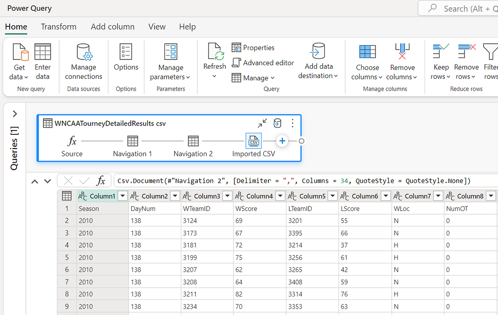
Now that the data is loaded we can start with some basic data preparation to get it into a format that we can use to create our features. The first thing we need to do is set the column names to be based on the first row of the dataset. This can be done by selecting the “Use first row as headers” option in either the Transform group on the Home ribbon or in the Transform menu item.
The next step is to rename the column “WLoc” to “location” by either selecting the column in the table view, or by right clicking on the column and selecting “Rename”.
The location column contains the location of the game, which is either “H” for home, “A” for away, or “N” for neutral. For our purposes, we want to convert this to a numerical value, where “H” is 1, “A” is -1, and “N” is 0, as this will make it easier to use in our model. This can be done by selecting the column and then using the Replace values… transform in the Transform menu item.

This will need to be done for the other two location values as well.
Finally, we need to change the data type of the location column to be a Whole number instead of Text. This can be done by selecting the column and then selecting the data type from the drop down list in the Transform group on the Home ribbon.

Instead of repeating the rename step for each of the location types, a little bit of M code can be used to replace the values in the location column. This can be done by selecting the previous transform in the query (Renamed columns) and then selecting the Insert step button in the formula bar. This will add a new step, and you can enter the following code to replace the values in the location column.
Table.ReplaceValue(#"Renamed columns", each [location], each if Text.Contains([location], "H") then "1" else if Text.Contains([location], "A") then "-1" else "0", Replacer.ReplaceText, {"location"})
We’ve got the data loaded, but it’s still not right for our model. Each row in the dataset represents a game between two teams, and includes the scores and statistics for both the winning and losing team in a single wide table. We need to create features that represent the performance of each team in the game and to have a row per team per game.
To do this we need to split the data into two tables, one for the winning team and one for the losing team. The simplest way to do this is to create a new query for each team and then merge them back together at the end. There are a few ways that this could be done, however to keep things simple and understandable (especially if we ever need to come back to this later), we will create two references to the source query and then append them together again, after doing some light transformations.
Referencing a column can be done either from the Queries panel on the left, or by selecting the context menu of the query if using Diagram view. This will create a new query that references the original query, and any changes made to the original query will be reflected in the new query. I did this twice, once for the winning team and once for the losing team and then renamed the columns by prefixing them with “T1_” and “T2_” respectively.
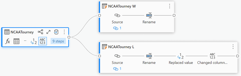
Once the column values are set, we can then combine the two queries back together by using Append Queries and then create our first feature, which is the point difference between the two teams. This can be done by selecting the T1_Score and T2_Score columns and then selecting “Subtract” from the “Standard” group on the Add column ribbon.
Now that’s done, we can then load the data into the Lakehouse as a new table. The final result should look something like this:

There are a few limitations with the no code approach, the main one is that it’s not easy to reuse queries or transformations. In the above example we would need to repeat the same steps another three times to load each of the individual csv files. This is where copy / paste comes in handy, but it’s not ideal. Let’s look at a low code approach next.
In the low code approach we will use a combination of the visual interface and the M language to load and transform the data. This approach is more flexible than the no code approach, but still doesn’t require a lot of code to be written.
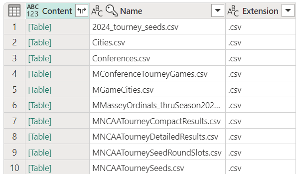
The goal of the low code approach is to reduce the number of repeated queries that are needed and to make it easier to reuse transformations. To do this we will take advantage of the fact that Power Query is a functional language and that we can create functions to encapsulate the transformations that we want to apply to the data. When we first loaded the data from the Lakehouse there were four steps that were created, the second step was to convert the contents of the Lakehouse into a table, with each row containing a reference to a binary csv file. We can use this as the input into a function, which will load the csv into a new table, using the Invoke custom function transformation for each row of the table.
To create the function, select “Blank query” from the Get data menu, or right click the Queries panel and select “New query” > “Blank query”. In the new query window, enter the following code:
(TableContents as binary) =>let
  Source = Csv.Document(TableContents, [Delimiter = ",", Columns = 34, QuoteStyle = QuoteStyle.None]),
  PromoteHeaders = Table.PromoteHeaders(Source, [PromoteAllScalars = true])
in
  PromoteHeaders
The code of this function has been copied from our initial no code approach, but instead of loading the csv file directly, it takes a parameter called TableContents, reads it as a csv file Csv.Document and then sets the first row of the data to be the column headers Table.PromoteHeaders.
We can then use the Invoke custom function transformation to apply this function to each row of the Lakehouse query. This can be done by selecting the “Invoke custom function” transformation from the Add column ribbon and then selecting the function that we just created.
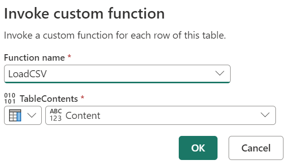
This will create a new column in the Lakehouse query, with the entire contents of the csv file loaded into a table, which is represented as [Table] in the table view. We can then use the expand function on the column heading to expand the table into individual columns.
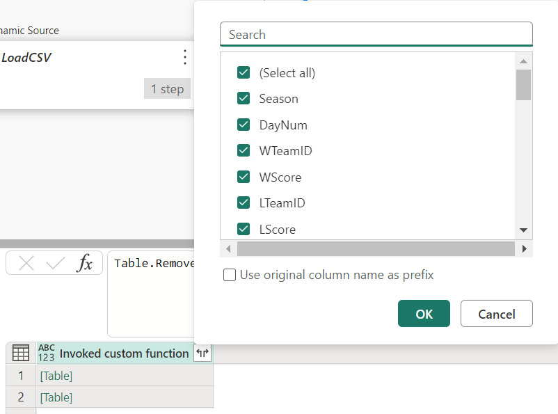
The result effectively combines the two csv files into a single table, which we can then continue to create our features from as before.
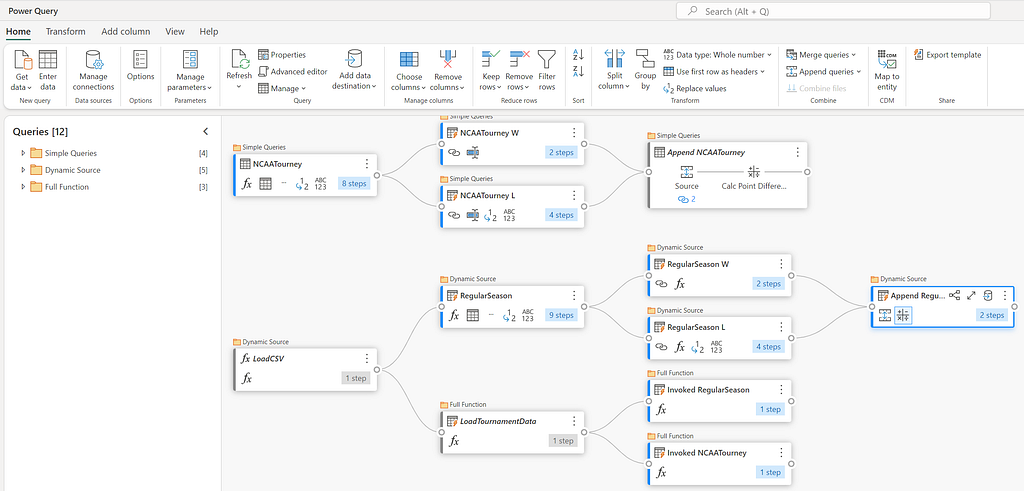
There are still some limitations with this approach, while we’ve reduced the number of repeated queries, we still need to duplicate everything for both the regular season and tournament games datasets. This is where the all code approach comes in.
The all code approach is the most flexible and powerful approach, but also requires the most amount of code to be written. This approach is best suited for those who are comfortable with writing code and want to have full control over the transformations that are applied to the data.
Essentially what we’ll do is grab all the M code that was generated in each of the queries and combine them into a single query. This will allow us to load all the csv files in a single query and then apply the transformations to each of them in a single step. To get all the M code, we can select each query and then click on the Advanced Editor from the Home ribbon, which displays all the M code that was generated for that query. We can then copy and paste this code into a new query and then combine them all together.
To do this, we need to create a new blank query and then enter the following code:
(TourneyType as text) => let
  Source = Lakehouse.Contents(null){[workspaceId = "..."]}[Data]{[lakehouseId = "..."]}[Data],
  #"Navigation 1" = Source{[Id = "Files", ItemKind = "Folder"]}[Data],
  #"Filtered rows" = Table.SelectRows(#"Navigation 1", each Text.Contains([Name], TourneyType)),
  #"Invoked custom function" = Table.AddColumn(#"Filtered rows", "Invoked custom function", each LoadCSV([Content])),
  #"Removed columns" = Table.RemoveColumns(#"Invoked custom function", {"Content", "Name", "Extension", "Date accessed", "Date modified", "Date created", "Attributes", "Folder Path", "ItemKind", "IsLeaf"}),
  #"Expanded Invoked custom function" = Table.ExpandTableColumn(#"Removed columns", "Invoked custom function", {"Season", "DayNum", "WTeamID", "WScore", "LTeamID", "LScore", "WLoc", "NumOT", "WFGM", "WFGA", "WFGM3", "WFGA3", "WFTM", "WFTA", "WOR", "WDR", "WAst", "WTO", "WStl", "WBlk", "WPF", "LFGM", "LFGA", "LFGM3", "LFGA3", "LFTM", "LFTA", "LOR", "LDR", "LAst", "LTO", "LStl", "LBlk", "LPF"}, {"Season", "DayNum", "WTeamID", "WScore", "LTeamID", "LScore", "WLoc", "NumOT", "WFGM", "WFGA", "WFGM3", "WFGA3", "WFTM", "WFTA", "WOR", "WDR", "WAst", "WTO", "WStl", "WBlk", "WPF", "LFGM", "LFGA", "LFGM3", "LFGA3", "LFTM", "LFTA", "LOR", "LDR", "LAst", "LTO", "LStl", "LBlk", "LPF"}),
  #"Renamed columns" = Table.RenameColumns(#"Expanded Invoked custom function", {{"WLoc", "location"}}),
  Custom = Table.ReplaceValue(#"Renamed columns", each [location], each if Text.Contains([location], "H") then "1" else if Text.Contains([location], "A") then "-1" else "0", Replacer.ReplaceText, {"location"}),
  #"Change Types" = Table.TransformColumnTypes(Custom, {{"Season", Int64.Type}, {"DayNum", Int64.Type}, {"WTeamID", Int64.Type}, {"WScore", Int64.Type}, {"LTeamID", Int64.Type}, {"LScore", Int64.Type}, {"location", Int64.Type}, {"NumOT", Int64.Type}, {"WFGM", Int64.Type}, {"WFGA", Int64.Type}, {"WFGM3", Int64.Type}, {"WFGA3", Int64.Type}, {"WFTM", Int64.Type}, {"WFTA", Int64.Type}, {"WOR", Int64.Type}, {"WDR", Int64.Type}, {"WAst", Int64.Type}, {"WTO", Int64.Type}, {"WStl", Int64.Type}, {"WBlk", Int64.Type}, {"WPF", Int64.Type}, {"LFGM", Int64.Type}, {"LFGA", Int64.Type}, {"LFGM3", Int64.Type}, {"LFGA3", Int64.Type}, {"LFTM", Int64.Type}, {"LFTA", Int64.Type}, {"LOR", Int64.Type}, {"LDR", Int64.Type}, {"LAst", Int64.Type}, {"LTO", Int64.Type}, {"LStl", Int64.Type}, {"LBlk", Int64.Type}, {"LPF", Int64.Type}}),
  Winners = Table.TransformColumnNames(#"Change Types", each if Text.StartsWith(_, "W") then Text.Replace(_, "W", "T1_") else Text.Replace(_, "L", "T2_")),
  #"Rename L" = Table.TransformColumnNames(#"Change Types", each if Text.StartsWith(_, "W") then Text.Replace(_, "W", "T2_") else Text.Replace(_, "L", "T1_")),
  #"Replaced Value L" = Table.ReplaceValue(#"Rename L", each [location], each if [location] = 1 then -1 else if Text.Contains([location], -1) then 1 else [location], Replacer.ReplaceValue, {"location"}),
  Losers = Table.TransformColumnTypes(#"Replaced Value L", {{"location", Int64.Type}}),
  Combined = Table.Combine({Winners, Losers}),
  PointDiff = Table.AddColumn(Combined, "PointDiff", each [T1_Score] - [T2_Score], Int64.Type)
in
  PointDiff
Note: the Lakehouse connection values have been removed
What’s happening here is that we’re:
Using the query is then as simple as selecting it, and then invoking the function with the TourneyType parameter.

This will create a new query with the function as it’s source, and the data loaded and transformed. It’s then just a case of loading the data into the Lakehouse as a new table.

As you can see, the LoadTournamentData function is invoked with the parameter “RegularSeasonDetailedResults” which will load both the Men’s and Women’s regular season games into a single table.
And that’s it!
Hopefully this post has given you a good overview of how to use Dataflow Gen2 to prepare data and create features for your machine learning model. Its low code approach makes it easy to create data pipelines quickly, and it contains a lot of powerful features that can be used to create complex transformations. It’s a great first port of call for anyone who needs to transform data, but more importantly, has the benefit of not needing to write complex code that is prone to errors, is hard to test, and is difficult to maintain.
At the time of writing, Dataflows Gen2 are unsupported with the Git integration, and so it’s not possible to version control or share the dataflows. This feature is expected to be released in Q4 2024.
Originally published at https://nobledynamic.com on April 15, 2024.
Feature Engineering with Microsoft Fabric and Dataflow Gen2 was originally published in Towards Data Science on Medium, where people are continuing the conversation by highlighting and responding to this story.
Originally appeared here:
Feature Engineering with Microsoft Fabric and Dataflow Gen2
Go Here to Read this Fast! Feature Engineering with Microsoft Fabric and Dataflow Gen2


Whether you are just starting up or aspiring to make another leap ensure that you are ready and your boss knows that
Originally appeared here:
How to Grow Your Career Without Feeling Stuck
Go Here to Read this Fast! How to Grow Your Career Without Feeling Stuck

Callbacks are an important functionality that helps with monitoring/debugging your pipelines. In this note, we cover the basics of callbacks and how to create custom ones for your use cases. More importantly, through examples, we also develop an understanding of the structure/componentization of LangChain pipelines and how that plays into the design of custom callbacks.
This note assumes basic familiarity with LangChain and how pipelines in LangChain work.
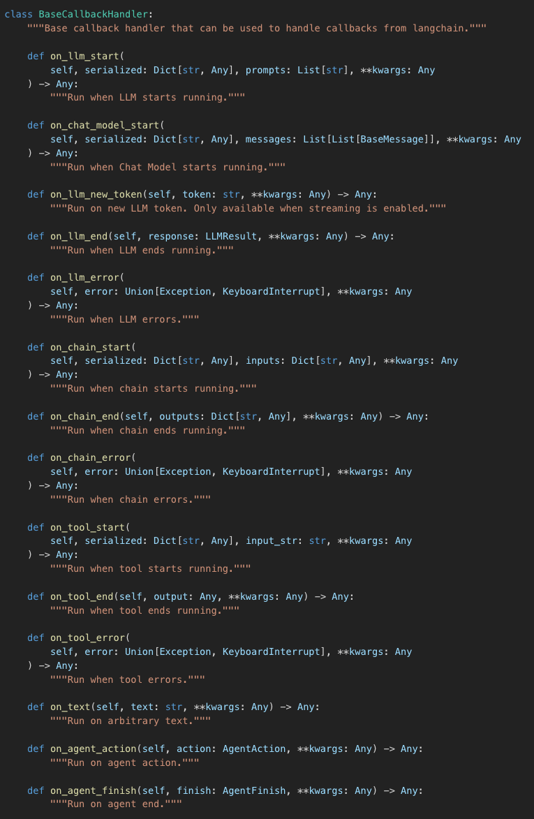
To learn about the basics of callbacks in LangChain, we start with the official documentation where we can find the definition of the BaseCallbackHandler class.
As you can see this is an abstract class that defines quite a few methods to cover various events in your LangChain pipeline. These methods can be grouped together into the following segments :
If you have worked with LangChain pipelines before, the methods along with their provided descriptions should be mostly self explanatory. For example, the on_llm_start callback is the event that gets triggered when the LangChain pipeline passes input to the LLM. And that on_llm_end is subsequently triggered when the LLM provides its final output.
NOTE : There are events triggers that can be used in addition to whats shown above. These can be found here. These cover triggers relating to Retrievers, Prompts, ChatModel etc.
Callbacks are a very common programming concept that have been widely used for a while now, so the high level concept of how callbacks work is well understood. So in this post, we focus on the specific nuances of how callbacks work in LangChain and how we could use it to satisfy our specific use cases.
Keeping in the mind the base Callback class that we saw in the previous section, we explore Callbacks in LangChain through a series of increasingly complex examples and in the process gain a better understanding of the structure of pipelines in LangChain. This would be a top-down approach to learning where we start with examples first and actual definitions later as I found that to be more useful personally for this specific topic.
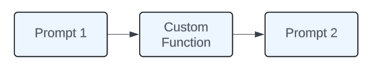
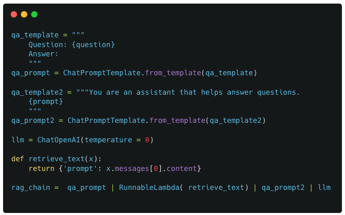
We start with a simple dummy chain that has 3 components : 2 prompts and a custom function to join them. I refer to this as a dummy example because its very unlikely that you would need two separate prompts to interact with each other, but it makes for an easier example to start with for understanding callbacks and LangChain pipelines.
Implementing this in code would look like :
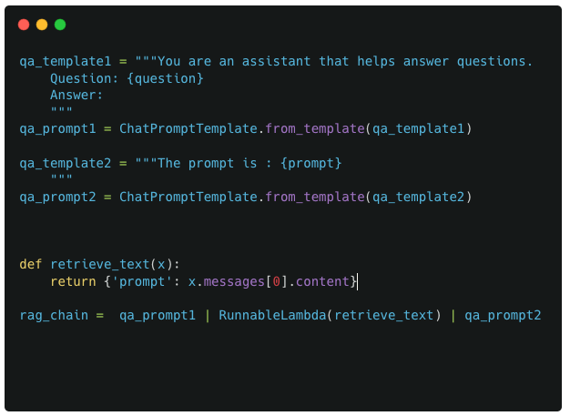
The above code is pretty textbook stuff. The only possibly complex piece is the retrieve_text and RunnableLambda function thats being used here. The reason this is necessary is because the format of the output from qa_prompt1 is not compatible with the format of the output required by qa_prompt2.
Defining the custom Callback
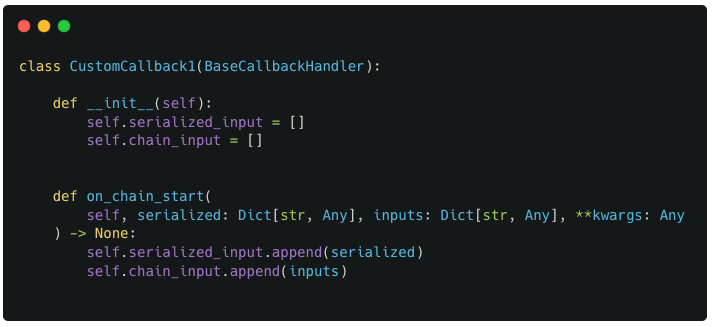
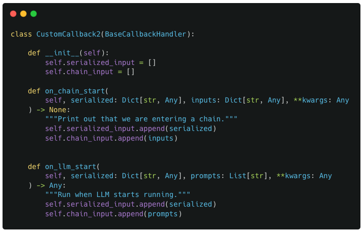
For our custom callback, we define a new subclass of BaseCallbackHandler called CustomCallback1 which defines the on_chain_start method. The method definition is straightforward as it simply takes the input values passed to it and saves it in 2 specific variables : chain_input and serialized_input
Invoking the custom callback

The above code shows one of the possible ways to pass your custom callback to your pipeline : As a list of callback objects as the value to a corresponding key of ‘callbacks’. This also makes it easy to guess that you can pass multiple callbacks to your LangChain pipeline.
Now comes the interesting part. After we have defined the callbacks and passed it on to our pipeline, we now perform a deep dive into the callback outputs
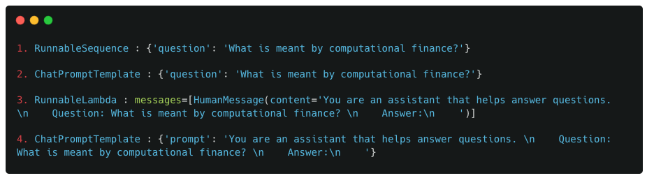
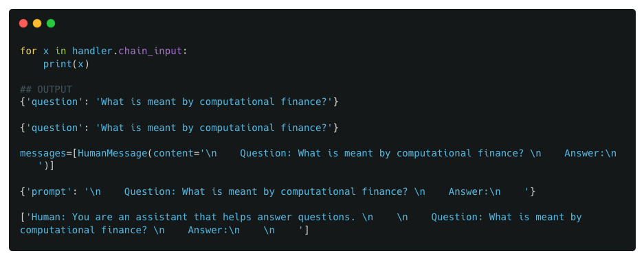
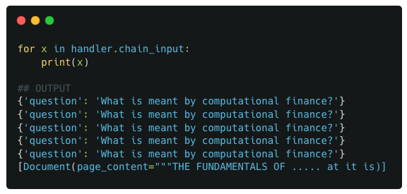
We first look at the values stored in chain_input
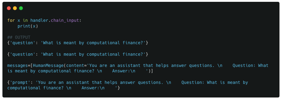
Observations :
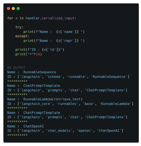
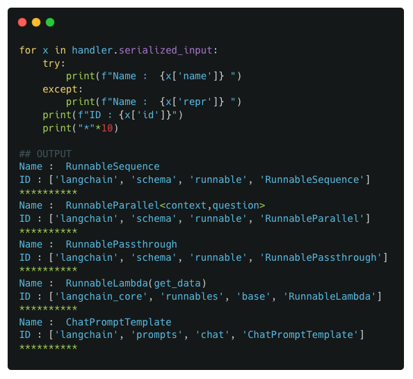
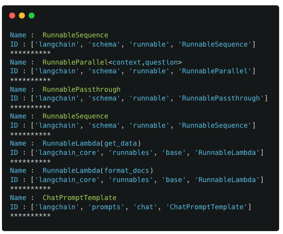
We next look at the outputs of serialized_input

Observations :
For the most part, the outputs seen in the chain_input and serialized_input make sense. Whether its the input values or the names/IDs of the components. The only largely unknown part is the RunnableSequence component, so we take a closer look at this.
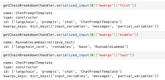
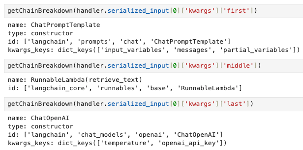
As I mentioned previously, the full contents of serialized_input is extensive and not easy to digest. So to make things easier, we look at only the high level attributes described in serialized_input and try to intrepret the results through these attributes. For this, we make use of a custom debugging function called getChainBreakdown (code in notebook).
We call getChainBreakdown on all values of serialized_input and observe the output. Specifically for the first RunnableSequence element, we look at the keys of the kwargs dict : first, midde, last, name.

On closer inspection of the kwargs argument and their values, we see that they have the same structure as our previous pipeline components. In fact, the first, middle and last components correspond exactly to the user-defined components of the pipeline.
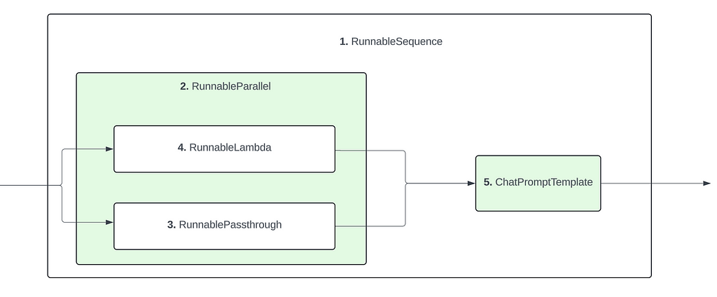
The above details form the basis of the final conclusion that we make here. That the structure of the pipeline is like shown below :
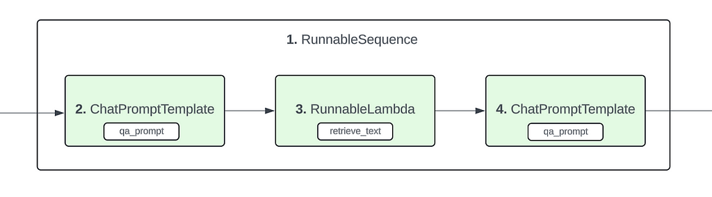
We do make a bit of a leap here as the above flowchart was confirmed after going through a bunch of examples and observing the format in which these components are created internally by LangChain. So bear with me as we go through these other examples which will solidify the conclusion that we make here.
With the above defined structure, the other pieces of the puzzle fit together quite well. Focusing on the chain_input values, lets map them to the components (with their ordering) defined above.
Observations :
The above breakdown shows how the structure of the pipeline described above fits perfectly with the data seen in serialized_input and chain_input
For the next example, we extend Example 1 by adding a LLM as the final step.
For the callback, since we have now added a LLM into the mix, we define a new custom callback that additionally defines the on_llm_start method. It has the same functionality as on_chain_start where the input arguments are saved into the callback object variables : chain_input and serialized_input
At this stage, instead of evaluating the callback variables, we switch things up and propose the potential structure of the pipeline. Given what we had learnt from the first example, the following should be the potential structure of the pipeline
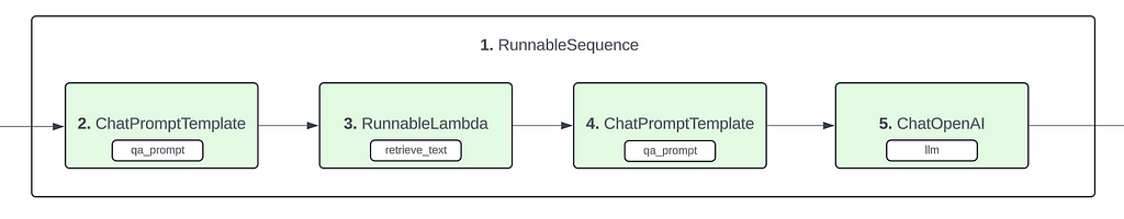
So we would have a RunnableSequence component as a wrapper for the pipeline. And additionally include a new ChatOpenAI object thats nested within the RunnableSequence component.
We now look at the values of in the callback object to validate the above proposed structure.
We first look at the values stored in chain_input
And then the serialized_input values :
As well as a deeper inspection of the RunnableSequence components
Observations :
By this stage, you should have an intuitive understanding of how LangChain pipelines are structured and when/how different callback events are triggered.
Though we have only focused on Chain and LLM events so far, these translate well to the other Tool and Agent triggers as well
For the next example, we progress to a more complex chain involving a parallel implementation (RunnableParallel)
The chain has a parallel implementation as its first block which computes two values : context and question, which are then passed on to a prompt template to create the final prompt. The parallel functionality is required because we need to pass both context and question to the prompt template at the same time, where the context is retrived from a different source while the question is provided by the user.
For the context value, we use a static function get_data that returns the same piece of text (this is a dummy version of an actual retriever used in RAG applications).

For the callback implementation, we use the same callback as the first example, CustomCallback1
Similar to previous examples, we start by looking at the outputs of chain_input and serialized_input
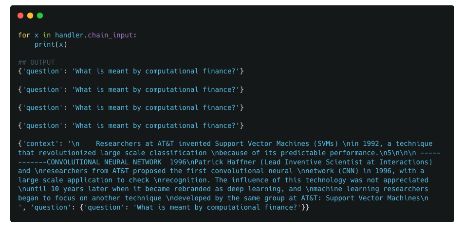
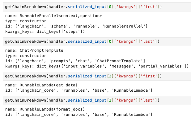
We also look do a deep dive into the RunnableSequence (index 0) and RunnableParallel (index 1) components

Observations :
Based on these observations, we can infer the final structure of the pipeline as such :
Same as Example 3, but with an additional processing function for retrieving context
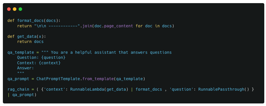
Similar to previous examples, we again look at the usual data points
We observe that there are now 2 RunnableSequence components in our pipeline. So for the next step, we deep dive into both of these RunnableSequence components to see its internal components
Observations :
In this case, the creation of the ‘context’ value can be considered a pipeline by itself as it involves 2 different components chained together. So any such sub-pipelines in your primary pipeline will be wrapped up by a RunnableSequence component
3. The values from chain_input also match up well with the pipeline components and their ordering (Not going to breakdown each component’s input here as it should be self-explanatory by now)
So based on the above observations, the following is the identified structure of this pipeline

The objective of this post was to help develop an (intuitive) understanding of how LangChain pipelines are structured and how callback triggers are associated with the pipeline.
By going through increasingly complex chain implementations, we were able to understand the general structure of LangChain pipelines and how a callback can be used for retrieving useful information. Developing an understanding of how LangChain pipelines are structured will also help facilitate the debugging process when errors are encountered.
A very common use case for callbacks is retrieving intermediate steps and through these examples we saw how we can implement custom callbacks that track the input at each stage of the pipeline. Add to this our understanding of the structure of the LangChain pipelines, we can now easily pinpoint the input to each component of the pipeline and retrieve it accordingly.
Notebook with code/examples : Contains few additional examples not covered in this note.
Unless specified otherwise, all images are created by the author.
In addition to Medium, I share my thoughts, ideas and other updates on Linkedin.
Callbacks and Pipeline structures in LangChain was originally published in Towards Data Science on Medium, where people are continuing the conversation by highlighting and responding to this story.
Originally appeared here:
Callbacks and Pipeline structures in LangChain
Go Here to Read this Fast! Callbacks and Pipeline structures in LangChain

Establishing causality is one of modern analytics’s most essential and often neglected areas. I would like to describe and highlight the tools most used in our causal inference workshop in an upcoming series of articles.
Let’s start by defining causal inference. I will use Scott Cunningham’s definition from the Mixtape book.
He defines it as the study of estimating the impact of events and choices on a given outcome of interest. We are trying to establish the cause-and-effect relationship between variables (we can call them treatment and effect). It is a widespread problem in many areas, from business to public policy settings.
Usually, the setup of the causality-finding framework is relatively simple and consists of:
This setup is not just a theoretical concept, but a practical tool that can be applied to a wide range of real-world scenarios. From website optimization to A/B testing, from drug clinical trials to estimating the effect of development programs, the applications of causal inference are vast and diverse.
Let’s consider the conditions we must meet to establish a causal effect. First, we must assume that the treatment and control groups are comparable. Both should behave the same when treated and when untreated. For example, objects from the treatment group should behave the same as those from the control group had they not been treated.
And vice versa, objects from the control group should behave the same as those from the treatment group had they been treated. Hence, the only difference between those groups comes solely from the treatment. Comparing the outcome in the treatment group to the outcome in the control group gives us the treatment effect.
The control group is not just a comparison but a counterfactual for the treatment group. It shows us how the former would have behaved had it not been exposed to a given treatment. This underscores the crucial role of the control group in establishing causal effects.
The assumption that both groups are similar is strong and depends on the available data and research design. Achieving this comparability is the crucial task of causal inference.
How can we obtain such conditions? Most articles tackling the topic of causality start with the notion that randomized experiments are the gold standard for establishing causality. However, they are often not feasible or practical to conduct.
Therefore, we are constantly looking for tools to help us find causal relationships. Research methods that tackle this problem are called quasi-experiments.
In the rest of the article, we will focus on one of the most important and often used quasi-experimental methods: difference-in-differences.
I will describe this method in the context of its classical application. To understand the approach, we will explore the work of Card and Kruger and their famous minimum wage study.
The effect of the minimum wage on employment is among the most heated debates in economics and public policy. The authors of the study tried to find an answer to this question. This type of problem is a perfect example of an issue we can’t explain using a randomized experiment. It would be practically impossible to randomly allocate certain groups or geographical regions to the different minimum wage levels.
In 1992, New Jersey increased the minimum wage from $4.25 to $5.05 per hour. Card and Kruger were looking for a benchmark against which to compare New Jersey.
Researchers decided to compare employment levels in New Jersey to those in Pennsylvania. The former state was chosen as the equivalent of a control group. They chose Pennsylvania because it is similar to New Jersey, both geographically and in terms of economic conditions.
They surveyed fast-food restaurants in both states before and after 1992 to check their number of employees. Scientists used employment in surveyed fast-food restaurants, as this business can quickly react to changes in the minimum wage.
Now’s the proper time to delve into the data. After the necessary data transformations (and simplifications for training purposes), we have the following data structure available. I used the data set from the David Card website (https://davidcard.berkeley.edu/data_sets.html):
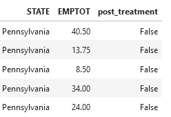
We can treat each row as the survey’s result in a restaurant. The crucial information is the state name, total employment, and the flag if the given record is from the period before or after the change in the minimum wage. We will treat the change in the minimum wage as a treatment variable in the analyzed study.
As a technical note, to make charting easier, we will store averages per time and state in a data frame:
How can we approach finding the effect of the minimum wage increase intuitively?
The most straightforward approach is to compare the average employment in both states after the treatment.

The chart shows that average employment in New Jersey was slightly lower than in Pennsylvania. Everyone who opposes the minimum wage is overjoyed and can conclude that this economic policy tool doesn’t work. Or is it perhaps too early to conclude?
Unfortunately, this approach is not correct. It omits crucial information about the pre-treatment differences in both states. The information we possess comes from something other than the randomized experiment, which makes it impossible to identify different factors that could account for the disparity between the two states.
These two states can be very different in terms of the number of people working there and the health of their economies. Comparing them after the treatment doesn’t reveal anything about the impact of the minimum wage and can result in inaccurate conclusions. I believe we should avoid this type of comparison in almost all cases.
We cannot draw conclusions based on comparing both states after the treatment. How about we look only at the state affected by the minimum wage change? Another way to evaluate the program’s impact is to compare employment in New Jersey before and after the change in the minimum wage. The chunk of code below does exactly this.

The before/after comparison presents a different picture. After raising the minimum wage, the average employment in fast-food restaurants in New Jersey increased.
Unfortunately, these conclusions are not definitive because this simple comparison has many flaws. The comparison between before and after the treatment makes one strong assumption: New Jersey’s employment level would have remained the same as before the change if the minimum wage had not increased.
Intuitively, it does not sound like a likely scenario. During this period, general economic activity had the potential to increase, government programs could have subsidized employment, and the restaurant industry could have experienced a significant surge in demand. Those are just some scenarios that could have influenced the employment level. It is typically not sufficient to establish the causal impact of the treatment by merely comparing the pre-and post-activity.
As a side note, this kind of comparison is quite common in various settings. Even though I think it’s more reliable than the previous approach we discussed, we should always be careful when comparing results.
Finally, we have all the necessary elements in place to introduce the star of the show, a difference-in-differences method. We found that we can’t just compare two groups after the treatment to see if there is a causal effect. Comparing the treated group before and after treatment is also not enough. What about combining the two approaches?
Difference-in-differences analysis allows us to compare the changes in our outcome variable between selected groups over time. The time factor is crucial, as we can compare how something has changed since the treatment started. This approach’s simplicity is surprising, but like all causal approaches, it relies on assumptions.
We will cover different caveats later. Let’s start with the components needed to perform this evaluation exercise. DiD study requires at least two groups at two distinct times. One group is treated, and the other is used as a comparison group. We have to know at what point to compare groups. What items do we require for the task at hand?
As the next step, we have to compute the following metrics:
And what are the next steps? We finally calculate the difference-in-differences, which is the difference between pre-treatment and post-treatment differences. This measure provides an estimate of the average treatment effect.
It’s easy to see the reasoning behind this strategy. The lack of data from the randomization experiment prevents us from comparing the differences between groups. However, it is possible to measure the difference between groups. A change in the difference in the outcome variable after treatment compared to the period before indicates a treatment effect.
Why is this? Before the treatment started, both groups had baseline values for the outcome variable. We assume that everything would have stayed the same in both groups if nothing had happened. However, the treatment occurred.
The treatment affected only one of the groups. Therefore, any changes in the outcome variable should only occur in the ‘treated’ group. Any change in the treatment group will change the outcome variable compared to the control group. This change is an effect of the treatment.
We assume the control group’s performance and trends will be the same as before treatment. Moreover, we must assume that the individuals in the treated group would have maintained their previous activity if the treatment had not occurred. The occurrence of treatment in one of the groups changes the picture and gives us the treatment effect.
We can investigate the effect of minimum wage with our new tool by returning to our minimum wage example. With the information we have, we can figure out these numbers:
Before the minimum wage increased, Pennsylvania’s average employment in fast-food restaurants was higher. It changed after the increase, and the average employment difference between the two states was much smaller.
The code below calculates the differences between employment before and after the increase in the minimum wage (nj_difference and penn_difference). We also calculate the difference-in-difference estimate by subtracting both differences.
The code below plots differences to provide a nice visual comparison. Additionally, I am adding the counterfactual line. Technically, it is an estimate of the post-treatment employment in New Jersey if it had followed Pennsylvania’s trend. We will discuss this line in the next paragraph, which is crucial for understanding the difference-in-differences.
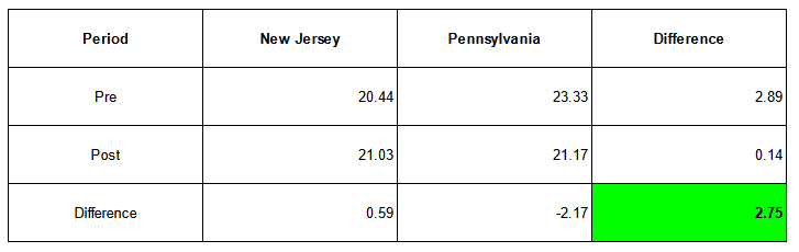
As you can see from the chart, the average employment in New Jersey increased by 0.59, while it decreased in Pennsylvania. Calculating the difference gives us an estimate of the treatment effect at 2.75. An increase in the minimum wage led to an increase in average employment, which is a surprising result.

Let us consider for a moment what caused these results. Employment in New Jersey did not increase significantly. However, the average employment rate in Pennsylvania decreased.
Without the minimum wage increase, we expect the average employment in New Jersey to follow the trend observed in Pennsylvania. If the minimum wage had not increased, average employment would have been lower.
On the chart, it is depicted as a counterfactual line, in which the New Jersey trend would follow the trend observed in Pennsylvania. The difference between the counterfactual line and the actual value observed in New Jersey equals the treatment effect of 2.75.
The introduction of the treatment changed this trend and allowed employment in New Jersey to maintain its value and slightly increase. What matters in this type of analysis is the change in magnitude of the treated group relative to the changes observed in the control group.
The table below summarizes the calculations in a format often encountered in DiD analysis. Treatment and control groups are represented in columns, the period in rows, and the measure of the outcome variable in cells.
The bottom-right corner displays the final estimate after calculating the differences.
I was writing about a simple calculation of a few averages. The difference-in-differences model’s computational simplicity is one of its advantages.
There are other ways to get those results. We could reach the same conclusions using a good, old linear regression. Expanding this model to multiple periods and groups would be beneficial.
One of the key advantages of the difference-in-differences model is its simplicity. We only need a handful of variables to run this model, making it straightforward and easy to use.
The model has the following form:

How can we interpret this model? B1 accounts for an increase in the value of the outcome variable when the treatment period starts. Our example shows the difference in the average employment in the control group after and before the treatment. We expect this change to happen without an increase in the minimum wage.
B2 accounts for a change in the outcome variable from the control to the treated group. It is the baseline difference between both groups — in a world before the treatment.
The interaction term (T*G) between the treatment period and the group shows the change in the outcome variable when both the treatment period and the treated group are activated. It has a value different from zero for a treated group in a treated period.
We want to achieve this in DiD analysis: the change of the outcome variable in the treated group during the treatment period compared to the control group.
There are many ways to calculate the results of this model in Python. For this example, we will use the statsmodels library. The specification of the linear model in our example looks like this:
As we can see in the regression output, the treatment effect (marked in yellow) is the same as calculated above. You can check that all the coefficients match the values calculated before.

It might seem like using regression analysis for simple average calculations is too much, but it has many benefits.
Firstly, the calculations are simpler than calculating averages for each group. We will also see the benefit of regression when we expand the model to include multiple comparison groups and periods.
What is also critical is that regression analysis allows us to assess the calculated parameters. We can obtain a confidence interval and p-value.
The results obtained by Card and Kruger were unexpected. They showed that an increase in the minimum wage does not negatively impact employment in the analyzed case. It even helped increase average employment.
This clever research indicates that we can find interesting and informative results even if we can’t do random experiments. It is the most fascinating aspect of causal inference that comes to mind when I think about it.
Regression analysis concludes the application of the difference-in-differences model. This demonstration demonstrates how powerful this method can be. Before we finish, let’s think about the potential limitations of this model.
As for most of the causal inference, the model is as good as our assumptions about it. In this method, finding the correct group for comparison is crucial and requires domain expertise.
Whenever you read about difference-in-differences, you will encounter parallel trend assumptions. This signifies that before the treatment, both groups had a consistent trend in the outcome variable. The model also requires that those trends continue in the same direction over time and that the difference between both groups in the outcome variable stays the same in the absence of treatment.
In our example, we assume that average employment in fast-food restaurants in both states changes in the same way with time. If this assumption is not met, then the difference-in-difference analysis is biased.
History is one thing, but we also assume that this trend will continue over time, and this is something we will never know and cannot test.
This assumption is only partially testable. We can take a look at historical trends to assess if they are similar to each other. To achieve this, we need more historical data — even plotting the trends across times gives a good indicator of this assumption.
It is only partially testable, as we can only assess the behavior of the treated group if they had received treatment. We assume the affected group would have behaved the same as our control group, but we can’t be 100% certain. There is only one world we can assess. It is the fundamental problem of causal inference.
The difference-in-differences also requires the structure of both groups to remain the same over time. We need both groups to have the same composition before the treatment. They should have the same characteristics, except for their exposure to the treatment.
At first glance, all the assumptions might make this method less appealing. But is there any statistical or analytical approach without assumptions? We have to get as much quality data as possible, make sensitivity analyses, and use domain knowledge anyway. Then, we can find fascinating insights using differences-in-differences.
The post above has one disadvantage (and potentially many more — please let me know). It covers a relatively simple scenario — two groups and two periods. In the upcoming posts, I’ll further complicate this picture by employing the same technique but in a more complex setting.
I hope this explanation of the difference-in-differences method will help everyone who reads it. This article is my first step in sharing my learning with causal inference. More will follow.
Card, David & Krueger, Alan B, 1994. “Minimum Wages and Employment: A Case Study of the Fast-Food Industry in New Jersey and Pennsylvania,” American Economic Review, American Economic Association, vol. 84(4), pages 772–793, September
https://davidcard.berkeley.edu/data_sets.html
Impact Evaluation in Practice — Second Edition https://www.worldbank.org/en/programs/sief-trust-fund/publication/impact-evaluation-in-practice
https://mixtape.scunning.com/09-difference_in_differences
Exploring causality in Python. Difference-in-differences was originally published in Towards Data Science on Medium, where people are continuing the conversation by highlighting and responding to this story.
Originally appeared here:
Exploring causality in Python. Difference-in-differences
Go Here to Read this Fast! Exploring causality in Python. Difference-in-differences


Climate change is a frustrating topic. Politicians are not committed to doing anything meaningful about it.
Originally appeared here:
Can AI “Fix” Climate Change? Perspective of a Data Nerd
Go Here to Read this Fast! Can AI “Fix” Climate Change? Perspective of a Data Nerd


Originally appeared here:
Uncover hidden connections in unstructured financial data with Amazon Bedrock and Amazon Neptune