Organizations are facing ever-increasing requirements for sustainability goals alongside environmental, social, and governance (ESG) practices. A Gartner, Inc. survey revealed that 87 percent of business leaders expect to increase their organization’s investment in sustainability over the next years. This post serves as a starting point for any executive seeking to navigate the intersection of generative […]
Explore the intricacies of the attention mechanism responsible for fueling the transformers
Attention! Attention!
Because ‘Attention is All You Need’.
No, I am not saying that, the Transformer is.
Image by author (Robtimus Prime seeking attention. As per my son, bright rainbow colors work better for attention and hence the color scheme.)
As of today, the world has been swept over by the power of transformers. Not the likes of ‘Robtimus Prime’ but the ones that constitute neural networks. And that power is because of the concept of ‘attention’. So, what does attention in the context of transformers really mean? Let’s try to find out some answers here:
First and foremost:
What are transformers?
Transformers are neural networks that specialize in learning context from the data. Quite similar to us trying to find the meaning of ‘attention and context’ in terms of transformers.
How do transformers learn context from the data?
By using the attention mechanism.
What is the attention mechanism?
The attention mechanism helps the model scan all parts of a sequence at each step and determine which elements need to be focused on. The attention mechanism was proposed as an alternative to the ‘strict/hard’ solution of fixed-length vectors in the encoder-decoder architecture and provide a ‘soft’ solution focusing only on the relevant parts.
What is self-attention?
The attention mechanism worked to improve the performance of Recurrence Neural Networks (RNNs), with the effect seeping into Convolutional Neural Networks (CNNs). However, with the introduction of the transformer architecture in the year 2017, the need for RNNs and CNNs was quietly obliterated. And the central reason for it was the self-attention mechanism.
The self-attention mechanism was special in the sense that it was built to inculcate the context of the input sequence in order to enhance the attention mechanism. This idea became transformational as it was able to capture the complex nuances of a language.
As an example:
When I ask my 4-year old what transformers are, his answer only contains the words robots and cars. Because that is the only context he has. But for me, transformers also mean neural networks as this second context is available to the slightly more experienced mind of mine. And that is how different contexts provide different solutions and so tend to be very important.
The word ‘self’ refers to the fact that the attention mechanism examines the same input sequence that it is processing.
There are many variations of how self-attention is performed. But the scaled dot-product mechanism has been one of the most popular ones. This was the one introduced in the original transformer architecture paper in 2017 — “Attention is All You Need”.
Where and how does self-attention feature in transformers?
I like to see the transformer architecture as a combination of two shells — the outer shell and the inner shell.
The outer shell is a combination of the attention-weighting mechanism and the feed forward layer about which I talk in detail in this article.
The inner shell consists of the self-attention mechanism and is part of the attention-weighting feature.
So, without further delay, let us dive into the details behind the self-attention mechanism and unravel the workings behind it. The Query-Key module and the SoftMax function play a crucial role in this technique.
This discussion is based on Prof. Tom Yeh’s wonderful AI by Hand Series on Self-Attention. (All the images below, unless otherwise noted, are by Prof. Tom Yeh from the above-mentioned LinkedIn post, which I have edited with his permission.)
So here we go:
Self-Attention
To build some context here, here is a pointer to how we process the ‘Attention-Weighting’ in the transformerouter shell.
Attention weight matrix (A)
The attention weight matrix A is obtained by feeding the input features into the Query-Key (QK) module. This matrix tries to find the most relevant parts in the input sequence. Self-Attention comes into play while creating the Attention weight matrix A using the QK-module.
How does the QK-module work?
Let us look at The different components of Self-Attention: Query (Q), Key (K) and Value (V).
I love using the spotlight analogy here as it helps me visualize the model throwing light on each element of the sequence and trying to find the most relevant parts. Taking this analogy a bit further, let us use it to understand the different components of Self-Attention.
Imagine a big stage getting ready for the world’s largest Macbeth production. The audience outside is teeming with excitement.
The lead actor walks onto the stage, the spotlight shines on him and he asks in his booming voice “Should I seize the crown?”. The audience whispers in hushed tones and wonders which path this question will lead to. Thus, Macbeth himself represents the role of Query (Q) as he asks pivotal questions and drives the story forward.
Based on Macbeth’s query, the spotlight shifts to other crucial characters that hold information to the answer. The influence of other crucial characters in the story, like Lady Macbeth, triggers Macbeth’s own ambitions and actions. These other characters can be seen as the Key (K) as they unravel different facets of the story based on the particular they know.
Finally, these characters provide enough motivation and information to Macbeth by their actions and perspectives. These can be seen as Value (V). The Value (V) pushes Macbeth towards his decisions and shapes the fate of the story.
And with that is created one of the world’s finest performances, that remains etched in the minds of the awestruck audience for the years to come.
Now that we have witnessed the role of Q, K, V in the fantastical world of performing arts, let’s return to planet matrices and learn the mathematical nitty-gritty behind the QK-module. This is the roadmap that we will follow:
Roadmap for the Self-Attention mechanism
And so the process begins.
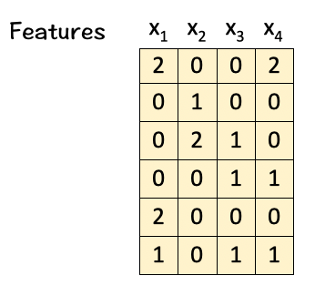
We are given:
A set of 4-feature vectors (Dimension 6)
Our goal :
Transform the given features into Attention Weighted Features.
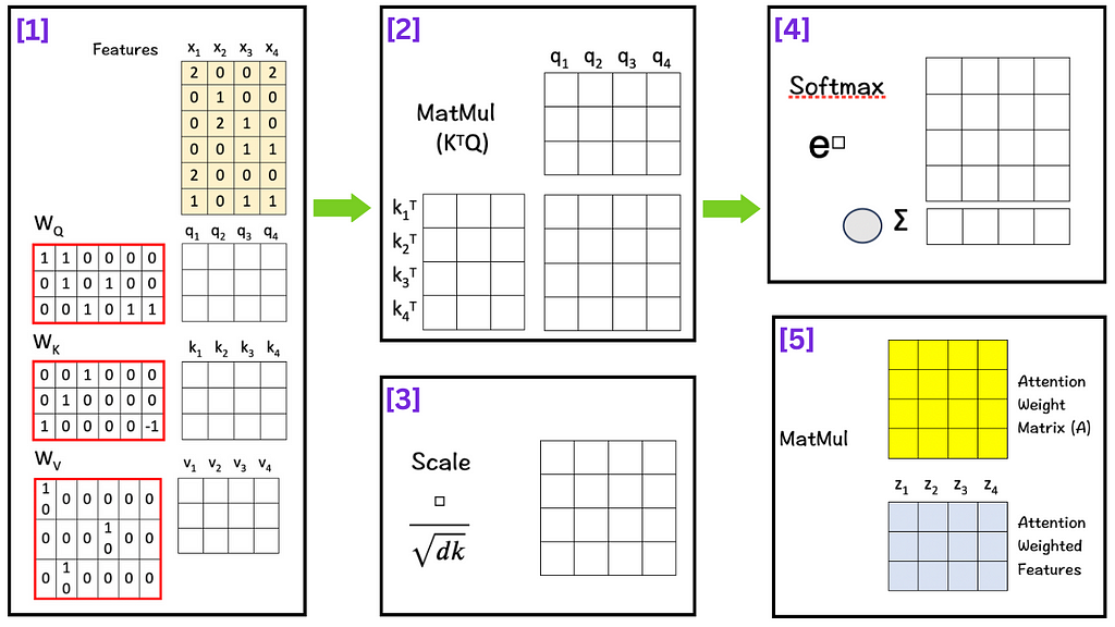
[1] Create Query, Key, Value Matrices
To do so, we multiply the features with linear transformation matrices W_Q, W_K, and W_V, to obtain query vectors (q1,q2,q3,q4), key vectors (k1,k2,k3,k4), and value vectors (v1,v2,v3,v4) respectively as shown below:
To get Q, multiply W_Q with X:
To get K, multiply W_K with X:
Similarly, to get V, multiply W_V with X.
To be noted:
As can be seen from the calculation above, we use the same set of features for both queries and keys. And that is how the idea of “self” comes into play here, i.e. the model uses the same set of features to create its query vector as well as the key vector.
The query vector represents the current word (or token) for which we want to compute attention scores relative to other words in the sequence.
The key vector represents the other words (or tokens) in the input sequence and we compute the attention score for each of them with respect to the current word.
[2] Matrix Multiplication
The next step is to multiply the transpose of K with Q i.e. K^T . Q.
The idea here is to calculate the dot product between every pair of query and key vectors. Calculating the dot product gives us an estimate of the matching score between every “key-query” pair, by using the idea of Cosine Similarity between the two vectors. This is the ‘dot-product’ part of the scaled dot-product attention.
Cosine-Similarity
Cosine similarity is the cosine of the angle between the vectors; that is, it is the dot product of the vectors divided by the product of their lengths. It roughly measures if two vectors are pointing in the same direction thus implying the two vectors are similar.
– If the dot product between the two vectors is approximately 1, it implies we are looking at an almost zero angle between the two vectors meaning they are very close to each other.
– If the dot product between the two vectors is approximately 0, it implies we are looking at vectors that are orthogonal to each other and not very similar.
– If the dot product between the two vectors is approximately -1, it implies we are looking at an almost an 180° angle between the two vectors meaning they are opposites.
[3] Scale
The next step is to scale/normalize each element by the square root of the dimension ‘d_k’. In our case the number is 3. Scaling down helps to keep the impact of the dimension on the matching score in check.
How does it do so? As per the original Transformer paper and going back to Probability 101, if two independent and identically distributed (i.i.d) variables q and k with mean 0 and variance 1 with dimension d are multiplied, the result is a new random variable with mean remaining 0 but variance changing to d_k.
Now imagine how the matching score would look if our dimension is increased to 32, 64, 128 or even 4960 for that matter. The larger dimension would make the variance higher and push the values into regions ‘unknown’.
To keep the calculation simple here, since sqrt [3] is approximately 1.73205, we replace it with [ floor(□/2) ].
Floor Function
The floor function takes a real number as an argument and returns the largest integer less than or equal to that real number.
The opposite of the floor function is the ceiling function.
This the ‘scaled’ part of the scaled dot-product attention.
[4] Softmax
There are three parts to this step:
Raise e to the power of the number in each cell (To make things easy, we use 3 to the power of the number in each cell.)
Sum these new values across each column.
For each column, divide each element by its respective sum (Normalize). The purpose of normalizing each column is to have numbers sum up to 1. In other words, each column then becomes a probability distribution of attention, which gives us our Attention Weight Matrix (A).
This Attention Weight Matrix is what we had obtained after passing our feature matrix through the QK-module in Step 2 in the Transformers section.
The Softmax step is important as it assigns probabilities to the score obtained in the previous steps and thus helps the model decide how much importance (higher/lower attention weights) needs to be given to each word given the current query. As is to be expected, higher attention weights signify greater relevance allowing the model to capture dependencies more accurately.
Once again, the scaling in the previous step becomes important here. Without the scaling, the values of the resultant matrix gets pushed out into regions that are not processed well by the Softmax function and may result in vanishing gradients.
[5] Matrix Multiplication
Finally we multiply the value vectors (Vs) with the Attention Weight Matrix (A). These value vectors are important as they contain the information associated with each word in the sequence.
And the result of the final multiplication in this step are the attention weighted features Zs which are the ultimate solution of the self-attention mechanism. These attention-weighted features essentially contain a weighted representationof the features assigning higher weights for features with higher relevance as per the context.
Now with this information available, we continue to the next step in the transformer architecture where the feed-forward layer processes this information further.
And this brings us to the end of the brilliant self-attention technique!
Reviewing all the key points based on the ideas we talked about above:
Attention mechanism was the result of an effort to better the performance of RNNs, addressing the issue of fixed-length vector representations in the encoder-decoder architecture. The flexibility of soft-length vectors with a focus on the relevant parts of a sequence was the core strength behind attention.
Self-attention was introduced as a way to inculcate the idea of context into the model. The self-attention mechanism evaluates the same input sequence that it processes, hence the use of the word ‘self’.
There are many variants to the self-attention mechanism and efforts are ongoing to make it more efficient. However, scaled dot-product attention is one of the most popular ones and a crucial reason why the transformer architecture was deemed to be so powerful.
Scaled dot-product self-attention mechanism comprises the Query-Key module (QK-module) along with the Softmax function. The QK module is responsible for extracting the relevance of each element of the input sequence by calculating the attention scores and the Softmax function complements it by assigning probability to the attention scores.
Once the attention-scores are calculated, they are multiplied with the value vector to obtain the attention-weighted features which are then passed on to the feed-forward layer.
Multi-Head Attention
To cater to a varied and overall representation of the sequence, multiple copies of the self-attention mechanism are implemented in parallel which are then concatenated to produce the final attention-weighted values. This is called the Multi-Head Attention.
Transformer in a Nutshell
This is how the inner-shell of the transformer architecture works. And bringing it together with the outer shell, here is a summary of the Transformer mechanism:
The two big ideas in the Transformer architecture here are attention-weighting and the feed-forward layer (FFN). Both of them combined together allow the Transformer to analyze the input sequence from two directions. Attention looks at the sequence based on positions and the FFN does it based on the dimensions of the feature matrix.
The part that powers the attention mechanism is the scaled dot-product Attention which consists of the QK-module and outputs the attention weighted features.
‘Attention Is really All You Need’
Transformers have been here for only a few years and the field of AI has already seen tremendous progress based on it. And the effort is still ongoing. When the authors of the paper used that title for their paper, they were not kidding.
It is interesting to see once again how a fundamental idea — the ‘dot product’ coupled with certain embellishments can turn out to be so powerful!
Image by author
P.S. If you would like to work through this exercise on your own, here are the blank templates for you to use.
Vaswani, Ashish, Noam Shazeer, Niki Parmar, Jakob Uszkoreit, Llion Jones, Aidan N. Gomez, Łukasz Kaiser, and Illia Polosukhin. “Attention is all you need.” Advances in neural information processing systems 30 (2017).
The LangChain documentation actually has a pretty good page on the high level concepts around its agents. It’s a short easy read, and definitely worth skimming through before getting started.
If you lookup the definition of AI Agents, you get something along the lines of “An entity that is able to perceive its environment, act on its environment, and make intelligent decisions about how to reach a goal it has been given, as well as the ability to learn as it goes”
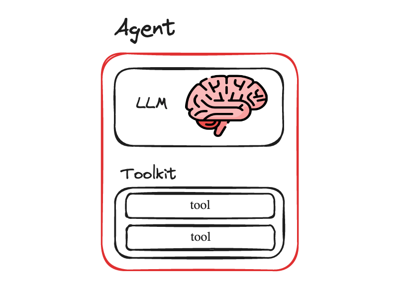
That fits the definition of LangChain agents pretty well I would say. What makes all this possible in software is the reasoning abilities of Large Language Model’s (LLM’s). The brains of a LangChain agent are an LLM. It is the LLM that is used to reason about the best way to carry out the ask requested by a user.
In order to carry out its task, and operate on things and retrieve information, the agent has what are called Tool’s in LangChain, at its disposal. It is through these tools that it is able to interact with its environment.
The tools are basically just methods/classes the agent has access to that can do things like interact with a Stock Market index over an API, update a Google Calendar event, or run a query against a database. We can build out tools as needed, depending on the nature of tasks we are trying to carry out with the agent to fulfil.
A collection of Tools in LangChain are called a Toolkit. Implementation wise, this is literally just an array of the Tools that are available for the agent. As such, the high level overview of an agent in LangChain looks something like this
Image by author
So, at a basic level, an agent needs
an LLM to act as its brain, and to give it its reasoning abilities
tools so that it can interact with the environment around it and achieve its goals
Building the Agent
To make some of these concepts more concrete, let’s build a simple agent.
We will create a Mathematics Agent that can perform a few simple mathematical operations.
The simplest place to start will be to fist define the tools for our Maths agent.
Let’s give it “add”, “multiply” and “square” tools, so that it can perform those operations on questions we pass to it. By keeping our tools simple we can focus on the core concepts, and build the tools ourselves, instead of relying on an existing and more complex tools like the WikipediaTool, that acts as a wrapper around the Wikipedia API, and requires us to import it from the LangChain library.
Again, we are not trying to do anything fancy here, just keeping it simple and putting the main building blocks of an agent together so we can understand how they work, and get our first agent up and running.
Let’s start with the “add” tool. The bottom up way to create a Tool in LangChain would be to extend the BaseTool class, set the name and description fields on the class, and implement the _run method. That would look like this
from langchain_core.tools import BaseTool

class AddTool(BaseTool):
    name = "add"
    description = "Adds two numbers together"
    args_schema: Type[BaseModel] = AddInput
    return_direct: bool = True

    def _run(
        self, a: int, b: int, run_manager: Optional[CallbackManagerForToolRun] = None
    ) -> str:
        return a + b
Notice that we need to implement the _run method to show what our tool does with the parameters that are passed to it.
Notice also how it requires a pydantic model for the args_schema. We will define that here
AddInput
    a: int = Field(description="first number")
    b: int = Field(description="second number")
Now, LangChain does give us an easier way to define tools, then by needing to extend the BaseTool class each time. We can do this with the help of the @tool decorator. Defining the “add” tool in LangChain using the @tool decorator will look like this
from langchain.tools import tool

@tool
def add(a: int, b: int) -> int:
 “””Adds two numbers together””” # this docstring gets used as the description
 return a + b # the actions our tool performs
Much simpler right. Behind the scenes, the decorator magically uses the method provided to extend the BaseTool class, just as we did earlier. Some thing to note:
the method name also becomes the tool name
the method params define the input parameters for the tool
the docstring gets converted into the tools description
Note that the description of a tool is very important as this is what the LLM uses to decide whether or not it is the right tool for the job. A bad description may lead to the not tool getting used when it should be, or getting used at the wrong times.
With the add tool done, let’s move on to the definitions for our multiply and square tools.
@tool
def multiply(a: int, b: int) -> int:
    """Multiply two numbers."""
    return a * b

@tool
def square(a) -> int:
    """Calculates the square of a number."""
    a = int(a)
    return a * a
And that is it, simple as that.
So we have defined our own three custom tools. A more common use case might be to use some of the already provided and existing tools in LangChain, which you can see here. However, at the source code level, they would all be built and defined using a similar methods as described above.
And that is it as far as our Tools our concerned. Now time to combine our tools into a Toolkit.
The Toolkit
Toolkits sound fancy, but they are actually very simple. They are literally just a a list of tools. We can define our toolkit as an array of tools like so
toolkit = [add, multiply, square]
And that’s it. Really straightforward, and nothing to get confused over.
Usually Toolkits are groups of tools that are useful together, and would be helpful for agents trying to carry out certain kinds of tasks. For example an SQLToolkit might contain a tool for generating an SQL query, validating an SQL query, and executing an SQL query.
The Integrations Toolkit page on the LangChain docs has a large list of toolkits developed by the community that might be useful for you.
The LLM
As mentioned above, an LLM is the brains of an agent. It decides which tools to call based on the question passed to it, what are the best next steps to take based on a tools description. It also decides when it has reached its final answer, and is ready to return that to the user.
Lastly we need a prompt to pass into our agent, so it has a general idea bout what kind of agent it is, and what sorts of tasks it should solve.
Our agent requires a ChatPromptTemplate to work (more on that later). This is what a barebones ChatPromptTemplate looks like. The main part we care about is the system prompt, and the rest are just the default settings we are required to pass in.
In our prompt we have included a sample answer, showing the agent how we want it to return the answer only, and not any descriptive text along with the answer
prompt = ChatPromptTemplate.from_messages(
    [
        ("system", """
          You are a mathematical assistant. Use your tools to answer questions.
          If you do not have a tool to answer the question, say so.

          Return only the answers. e.g
          Human: What is 1 + 1?
          AI: 2
          """),
        MessagesPlaceholder("chat_history", optional=True),
        ("human", "{input}"),
        MessagesPlaceholder("agent_scratchpad"),
    ]
)
That is it. We have setup our Tools and Toolkit, which our agent will need as part of its setup, so its knows what are the types of actions and capabilities it has at its disposal. And we have also setup the LLM and system prompt.
Now for the fun part. Setting up our Agent!
The Agent
LangChain has a number of different agents types that can be created, with different reasoning powers and abilities. We will be using the most capable and powerful agent currently available, the OpenAI Tools agent. As per the docs on the the OpenAI Tools agent, which uses newer OpenAI models also,
Newer OpenAI models have been fine-tuned to detect when one or more function(s) should be called and respond with the inputs that should be passed to the function(s). In an API call, you can describe functions and have the model intelligently choose to output a JSON object containing arguments to call these functions. The goal of the OpenAI tools APIs is to more reliably return valid and useful function calls than what can be done using a generic text completion or chat API.
In other words this agents is good at generating the correct structure for calling functions, and is able to understand if more than one function (tool) might be needed for our task also. This agent also has the ability to call functions (tools) with multiple input parameters, just like ours do. Some agents can only work with functions that have a single input parameter.
If you are familiar with OpenAI’s Function calling feature, where we can use the OpenAI LLM to generate the correct parameters to call a function with, the OpenAI Tools agent we are using here is leveraging some of that power in order to be able to call the correct tool, with the correct parameters.
In order to setup an agent in LangChain, we need to use one of the factory methods provided for creating the agent of our choice.
The factory method for creating an OpenAI tools agent is create_openai_tools_agent(). And it requires passing in the llm, tools and prompt we setup above. So let’s initialise our agent.
Finally, in order to run agents in LangChain, we cannot just call a “run” type method on them directly. They need to be run via an AgentExecutor.
Am bringing up the Agent Executor only here at the end as I don’t think it’s a critical concept for understanding how the agents work, and bring it up at the start with everything else would just the whole thing seem more complicated than it needs to be, as well as distract from understanding some of the other more fundamental concepts.
So, now that we are introducing it, an AgentExecutor acts as the runtime for agents in LangChain, and allow an agent to keep running until it is ready to return its final response to the user. In pseudo-code, the AgentExecutor’s are doing something along the lines of (pulled directly from the LangChain docs)
So they are basically a while loop that keep’s calling the next action methods on the agent, until the agent has returned its final response.
So, let us setup our agent inside the agent executor. We pass it the agent, and must also pass it the toolkit. And we are setting verbose to True so we can get an idea of what the agent is doing as it is processing our request
And that is it. We are now ready to pass commands to our agent
result = agent_executor.invoke({"input": "what is 1 + 1"})
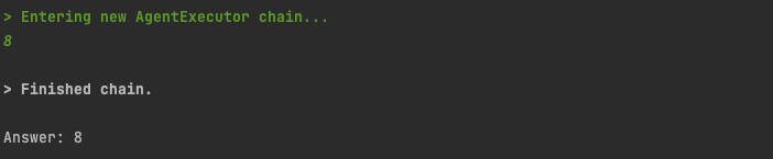
Let run our script, and see the agent’s output
python3 math-agent.py
Image by author
Since we have set verbose=True on the AgentExecutor, we can see the lines of Action our agent has taken. It has identified we should call the “add” tool, called the “add” tool with the required parameters, and returned us our result.
This is what the full source code looks like
import os
from langchain.agents import AgentExecutor, create_openai_tools_agent from langchain_openai import ChatOpenAI
from langchain.tools import BaseTool, StructuredTool, tool from langchain_core.prompts import ChatPromptTemplate, MessagesPlaceholder
os.environ["OPENAI_API_KEY"] = "sk-"
# setup the tools @tool def add(a: int, b: int) -> int: """Add two numbers.""" return a + b
@tool def multiply(a: int, b: int) -> int: """Multiply two numbers.""" return a * b
@tool def square(a) -> int: """Calculates the square of a number.""" a = int(a) return a * a
prompt = ChatPromptTemplate.from_messages( [ ("system", """You are a mathematical assistant. Use your tools to answer questions. If you do not have a tool to answer the question, say so.
Return only the answers. e.g Human: What is 1 + 1? AI: 2 """), MessagesPlaceholder("chat_history", optional=True), ("human", "{input}"), MessagesPlaceholder("agent_scratchpad"), ] )
# Choose the LLM that will drive the agent llm = ChatOpenAI(model="gpt-3.5-turbo-1106", temperature=0)
# setup the toolkit toolkit = [add, multiply, square]
# Create an agent executor by passing in the agent and tools agent_executor = AgentExecutor(agent=agent, tools=toolkit, verbose=True)
result = agent_executor.invoke({"input": "what is 1 + 1?"})
print(result['output'])
Testing our agent
Let’s shoot a few questions at our agent to see how it performs.
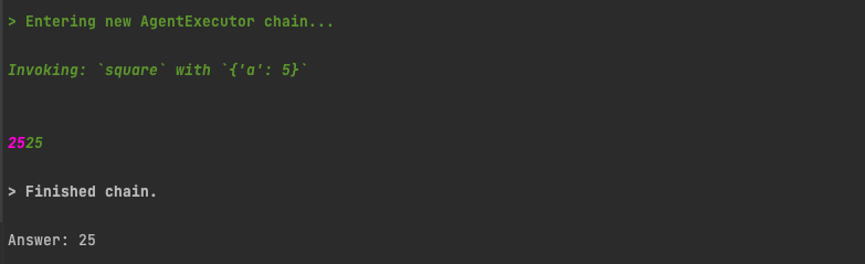
what is 5 squared?
Again we get the correct result, and see that it does use our square tool
Image by author
what is 5 to the power of 6?
It takes an interesting course of action. It first uses the square tool. And then, using the result of that, tries to use the multiply tool a few times to get the final answer. Admittedly, the final answer, 3125, is wrong, and needs to be multiplied by 5 one more time to get the correct answer. But it is interesting to see how the agent tried to use different tools, and multiple steps to try and get to the final answer.
Image by author
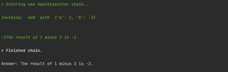
what is 1 minus 3?
We don’t have a minus tool. But it is smart enough to use our add tool, but set the second value to -3. Its funny and somewhat amazing sometimes how they are smart and creative like that.
Image by author
what is the square root of 64
As a final test, what if we ask it to carry out a mathematical operation that is not part of our tool set? Since we have no tools for square rooting, it does not attempt to call a tool, and instead calculates the value directly using just the LLM.
Image by author
Our system prompt did tell it to answer that it “does not know” if it does not have the correct tool for the job, and it did do that sometimes during testing. An improved initial system prompt could probably help resolve that, at least to some extent
Observations
Based on using the agent a bit, I noticed the following
when asking it direct questions which it had the tools to answer with, it was pretty consistent at using the correct tools for the job, and returning the correct answer. So, pretty reliable in that sense.
if the question is a little complicated, for example our “5 to the power of 6” question, it does not always return the correct results.
it can sometimes use just the pure power of the LLM to answer our question, without invoking our tools.
The Future
Agents, and programs that can reason from themselves, are a new paradigm in programming, and I think they are going to become a much more mainstream part of how lots of things are built. Obviously the non-deterministic (i.e not wholly predictable) nature of LLM’s means that agents results will also suffer from this, questioning how much we can rely on them for tasks where we need to be sure of the answers we have.
Perhaps as the technology matures, their results can be more and more predictable, and we may develop some work arounds for this.
I can also see agent type libraries and packages starting to become a thing. Similar to how we install third party libraries and packages into software, for example via the pip package manager for python, or Docker Hub for docker images, I wonder if we may start to see a library and package manager of agents start being developed, with agents developed that become very good at their specific tasks, which we can then also install as packages into out application.
Indeed LangChain’s library of Toolkits for agents to use, listed on their Integrations page, are sets of Tools built by the community for people to use, which could be an early example of agent type libraries built by the community.
Conclusion
Hope this was a useful introduction into getting you started building with agents in LangChain.
Remember, agents are basically just a brain (the LLM), and a bunch of tools, which they can use to get stuff done in the world around us.
Happy hacking!
If you enjoyed the article, and would like to stay up to date on future articles I release about building things with LangChain and AI tools, do subscribe here to be notified by email when they come out
It’s no secret that much of the success of LLMs still depends on our ability to prompt them with the right instructions and examples. As newer generation LLMs become more and more powerful, prompts have become complex enough to be considered programs themselves. These prompt programs are a lot like recipes — both have a set of instructions to follow and transform raw materials, be it data or ingredients.
Prompt engineering is thus similar to improving a recipe. Home chefs will often stick to the overall recipe but make some small changes — for example leaving out garlic or adding parsley in a pasta dish. Frameworks like DSPy are following this overall paradigm when they optimize the in-context examples. Pro-level chefs, however, use the recipe as inspiration, and often re-interpret components of the dish completely. For example, they might see spaghetti in pasta dish as the starchy component and might swap it for freshly made gnocchi to achieve a similar composition.
What is it that allows pro-level chefs to work so creatively? It’s that they think about recipes in an abstract way, like in the pasta example above. Manual prompt engineering is similar to pro-level cooking. It can get impressive results but requires a lot of time and knowledge. What we really want is the creativity of manual prompt engineering but without the effort.
The power of abstract prompts
Let’s say we want to improve a prompt for labeling speaker responses. We’ll eventually run it with many different inputs, but plug in a concrete one for now:
Instructions: Does Speaker 2's answer mean yes or no?
Output labels: no, yes
Input: Speaker 1: "You do this often?" Speaker 2: "It's my first time."
Output:
Assume, for a moment, that we had an abstract representation of this prompt that pulls out its separate components and is easy to manipulate. Maybe something like this:
A simple prompt for a classification task represented as an abstract symbolic program. Image by author.
With this, you could automate a lot of the (semi)-manual tinkering you have to do during prompt prototyping. Making small edits such as paraphrasing would be just the start. Want to try out Chain-of-Thought reasoning? Add a paragraph that says “Let’s think step-by-step.” How about changing the data formatting to JSON? Simply change the formatattribute of the InputData parameters. You can also explore
Going from single examples to batch annotation
Changing your retriever and ranking function in a RAG scenario
Re-ordering some of the paragraphs
Compressing certain parts of the instructions
Etc.
Essentially, plug in your favorite prompt engineering heuristic. This abstract representation of prompts allows us to truly get creative and automatically explore a large space of possible prompts. But how can we represent prompts as abstract and modifiable programs in Python? Read on.
Turning prompts into abstract programs
“Any problem in computer science can be solved by another layer of indirection.”
To represent abstract prompts, let’s first convert it into a non-symbolic prompt program by breaking them into individual components, implemented as Python classes:
class Component: def __init__(self, **kwargs): pass class Metaprompt(Component): pass class Paragraph(Component): pass class InputData(Component): pass
So far, so good. It’s similar to what DSpy does, albeit more general as we also represent the internal structure of a prompt.
Next, we turn it into a symbolic prompt program so that we canmake arbitrary changes (this is also beyond static DSPy programs). This can be done with pyGlove, a library for symbolic object-oriented programming (SOOP). pyGlove turns Python classes into manipulable, symbolic objects whose properties remain fully editable after instantiation.
With pyGlove, all we need to do is add the pg.symbolize decorator:
import pyglove as pg
@pg.symbolize
class Component:
    def __init__(self, **kwargs): pass
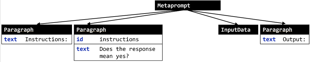
We can now query and modify prompt programs via a whole host of specifiers, similar to working with a DOM tree. Let’s say we’d like to transform our program above into the following:
The target prompt program we want to achieve. Image by author.
Note that we’re now asking “Does the response mean yes?” and not providing output labels of yes and no. To get there, we need to (i) change the instruction text and (ii) delete the third node. With pyGlove, this is very easy:
prompt.rebind({'children[1].text': 'Does the response mean yes?'})
prompt.rebind({'children[2]': pg.MISSING_VALUE})
print(prompt)
The printout confirms that we’re successful:
Metaprompt(
  children = [
    0 : Paragraph(
      text = 'Instructions: '
    ),
    1 : Paragraph(
      id = 'instructions',
      text = 'Does the response mean yes?'
    ),
    2 : InputData(),
    3 : Paragraph(
      text = 'Output: '
    )
  ]
)
Voilà! Essentially, pyGlove gives us a way to work with Python classes (and functions) as if they were still source code with little overhead. Now that we have flexible and easily manipulable representations, let’s put them to use.
Wait a minute. We might have a way to represent and modify prompts now, but we’re still missing a process to optimize them automatically.
Once chefs understand the abstraction and components of a recipe, they’ll try out many variants, refining the taste, cost, or presentation, until it feels right. To do the same with prompt abstractions, we need a search algorithm, an objective as well as set of labeled samples to know that we’re making progress.
Sounds like a lot to implement yourself? Meet SAMMO, a Python library for building and optimizing symbolic prompt programs.
Warming up: Instruction tuning with SAMMO
To illustrate SAMMO’s core workflow, we’ll now show how to tune the instructions part of our prompt example from above. Once we’ve worked through this toy example, we’ll be ready to discuss more advanced applications, like RAG optimization or compression.
The key steps are
Defining your starting prompt
Getting the data ready — a few hundred labeled examples are enough.
Defining the objective
Choosing a set of mutators
Running the optimization
Step 1: Defining your starting prompt
We’ve pretty much already done this above. SAMMO expects a function, so we’ll have to wrap it in one. If you’d like to store extra information, wrap it in a Callable instead. We’ll also wrap it in an Output component to run it.
Here is where you can be as creative as you’d like. You can implement your own operators that generate new prompt variants, or simply rely on the pre-built mutation operators that SAMMO offers.
Below, we do the latter and go for a mix of paraphrasing and inducing instructions from a few labeled examples, essentially implementing Automatic Prompt Engineering (APE).
The introductory example prompt was actually taken from the BigBench implicatures task which we’ll use to run this experiment. If you run the optimization with 100 samples for training and testing and a budget of 48 candidates evaluations, you’ll see that SAMMO improves the starting prompt accuracy from 0.56 to 0.77 — a 37.5% improvement. What instructions worked best?
...
Paragraph(
    "Consider the dialogue, context, and background "
    "information provided to determine the most suitable output label",
    id="instructions",
)
...
Interestingly, different LLMs prefer quite different instructions. GPT-3.5 liked generic instructions the best as seen above. Llama-2’s best prompt selected by SAMMO with the same training and budget setup used an empty string in the instructions part:
...
Paragraph(
    "",
    id="instructions",
)
...
Getting practical: RAG tuning
We’ll now show how to convert a RAG pipeline into a symbolic program and tune it with SAMMO. We’ll use semantic parsing as our application task where we want to translate user queries into domain-specific language (DSL) constructs, for example, to query some database or call an external API.
To create the starting prompt, we include a list of all operators, use an embedding-based retriever to get five fewshot examples and then instruct the LLM to output its answer in the same format as the examples.
def __call__(self, return_raw=False): structure = [ Section("Syntax", self._dtrain.constants["list_of_operators"]), Section( "Examples", EmbeddingFewshotExamples( self._embedding_runner, self._examples, 5 ), ), Section( "Complete and output in the same format as above", InputData(), ), ] instructions = MetaPrompt( structure, render_as="markdown", data_formatter=JSONDataFormatter(), ) return Output( instructions.with_extractor(), on_error="empty_result", )
Now that we have a symbolic program, let’s get creative. For the mutations, we explore
varying numbers of fewshot examples
different formats (XML, JSON, line-by-line) for the fewshot examples
providing additional information about the DSL or not
showing input-output pairs or groups of inputs and outputs
Running SAMMO with these and a total budget of 24 candidates to try out, we can see a clear trend. Below are test set accuracies for three different datasets across four different LLMs. In the overwhelming majority of cases, we can see that SAMMO can lift performance substantially, even for the highest-performing LLMs.
Even with a small budget of 24 candidates evaluations we can get major lifts in performance. Image by author.
Conclusions
Converting your prompts into symbolic programs is a really powerful idea to explore a large design space of possible prompts and settings. Just as a pro-level chef deconstructs and reinterprets recipes to create culinary innovations, symbolic programming lets us apply the same level of creativity and experimentation to automatic prompt engineering.
SAMMO implements symbolic program search through a set of mutation operators and search routine. Empirically, this can translate into large improvements in accuracy for both instruction tuning and RAG tuning, independent of the backend LLM.
You can extend SAMMO with custom mutation operators to include your favorite prompt engineering techniques or implement objectives to go beyond accuracy (e.g., cost). Happy prompt cooking!
A deep dive into biases in machine learning, with a focus on historical (or social) biases.
Humans are biased. To anyone who has had to deal with bigoted individuals, unfair bosses, or oppressive systems — in other words, all of us — this is no surprise. We should thus welcome machine learning models which can help us to make more objective decisions, especially in crucial fields like healthcare, policing, or employment, where prejudiced humans can make life-changing judgements which severely affect the lives of others… right? Well, no. Although we might be forgiven for thinking that machine learning models are objective and rational, biases can be in-built into models in a myraid of ways. In this blog post, we will be focusing on historical biases in machine learning (ML).
ML models suffer from statistical biases since statistics play a big role in how they work. However, these models are also designed by humans, and use data generated by humans for training, making them vulnerable to learning and perpetuating human biases. Thus, perhaps counterintuitively, ML models are arguably more susceptible to biases than humans, not less.
Experts disagree on the exact number of algorithmic biases, but there are at least 7 potential sources of harmful bias (Suresh & Guttag, 2021), each generated at a different point in the data analysis pipeline:
Historical bias, which arises from the world, in the data generation phase;
Representation bias, which comes about when we take samples of data from the world;
Measurement bias, where the metrics we use or the data we collect might not reflect what we actually want to measure;
Aggregation bias, where we apply the same approach to our whole data set, even though there are subsets which need to be treated differently;
Learning bias, where the ways we have defined our models cause systematic errors;
Evaluation bias, where we ‘grade’ our models’ performances on data which does not actually reflect the population we want to use the models on, and finally;
Deployment bias, where the model is not used in the way the developers intended for it to be used.
While all of these are important biases, which any budding data scientist should consider, today I will be focusing on historical bias, which occurs at the first stage of the pipeline.
Psst! Interested in learning more about other types of biases? Watch this helpful video:
Historical Bias
Unlike the other types of biases, historical bias does not originate from ML processes, but from our world. Our world has historically been, and still is peppered with prejudices, so even when the data we use to train our models perfectly reflects the world we live in, our data might capture these discriminatory patterns. This is where historical bias arises. Historical bias may also manifest in instances where our world has made strides towards equality, but our data does not adequately capture these changes, reflecting past inequalities instead.
Why Should We Care?
Most societies have anti-discrimination laws, which aim to protect the rights of vulnerable groups in society, who have been historically oppressed. If we are not careful, previous acts of discrimination might be learned and perpetuated by our ML models due to historical bias. With the rising prevalence of ML models in practically every area of our lives, from the mundane to the life-changing, this poses a particularly insidious threat — historically biased ML models have the potential to perpetuate inequality on a never-before-seen scale. Data scientist and mathematician Cathy O’Neil calls such models ‘weapons of math destruction’ or WMDs for short — models whose workings are a mystery, generate harmful outcomes which victims cannot dispute, and which often penalise the poor and oppressed in our society, while benefiting those who are already well off (O’Neil, 2017).
Such WMDs are already impacting vulnerable groups worldwide. Although we would think that Amazon, which profits from recommending us items we have never heard of, yet suddenly desperately want, would have mastered machine learning, it was found that an algorithm they used to scan CVs had learned a gender bias, due to the historically low number of women in tech. Perhaps more chillingly, predictive policing tools have also been shown to have racial biases, as have algorithms used in healthcare, and even the courtroom. The mass proliferation of such tools obviously has great impacts, particularly since they may serve as a way to entrench the already deep-rooted inequalities in our society. I would argue that these WMDs are a far greater hindrance in our collective efforts to stamp out inequality compared to biased humans, for two main reasons:
Firstly, it is hard to get insight into why ML models make certain predictions. Deep learning seems to be the buzzword of the season, with complicated neural networks taking the world by storm. While these models are exciting since they have the potential to model very complex phenomena which humans cannot understand, they are considered black-box models, since their workings are often opaque, even to their creators. Without concerted efforts to test for historical (and other) biases, it is difficult to tell if they are inadvertently discriminating against protected groups.
Secondly, the scale of damage which might be done by a historically biased model is, in my opinion, unprecedented and overlooked. Since humans have to rest, and need time to process information effectively, the damage a single prejudiced person might do is limited. However, just one biased ML model can pass thousands of discriminatory judgements in a matter of minutes, without resting. Dangerously, many also believe that machines are more objective than humans, leading to reduced oversight over potentially rogue models. This is especially concerning to me, since with the massive success of large language models like ChatGPT, more and more people are developing an interest in implementing ML models into their workflows, potentially automating the rise of WMDs in our society, with devastating consequences.
What Can We Do About It?
While the impacts of biased models might be scary, this does not mean that we have to abandon ML models entirely. Artificial Intelligence (AI) ethics is a growing field, and researchers and activists alike are working towards solutions to get rid of, or at least reduce the biases in models. Notably, there has been a recent push for FAT or FATE AI — fair, accountable, transparent and ethical AI, which might help in the detection and correction of biases (among other ethical issues). While it is not a comprehensive list, I will provide a brief overview of some ways to mitigate historical biases in models, which will hopefully help you on your own data science journey.
Statistical Solutions
Since the problem arises from disproportionate outcomes in the real world’s data, why not fix it by making our collected data more proportional? This is one statistical approach of dealing with historical bias, suggested by Suresh, H., & Guttag, J. (2021). Put simply, it comprises collecting more data from some groups and less from others (systematic over- or under- sampling), resulting in a more balanced distribution of outcomes in our training dataset.
Model-based Solutions
In line with the goals of FATE AI, interpretability can be built into models, making their decision-making processes more transparent. Interpretability allows data scientists to see why models make the decisions they do, providing opportunities to spot and mitigate potential instances of historical biases in their models. In the real world, this also means that victims of machine-based discrimination can challenge decisions made by previously inscrutable models, and hopefully cause them to be reconsidered. This will hopefully increase trust in our models.
More technically, algorithms and models to address biases in ML models are also being developed. Adversarial debiasing is one interesting solution. Such models essentially consist of two parts: a predictor, which aims to predict an outcome, like hireability, and an adversary, which tries to predict protected attributes based on the predicted outcomes. Like boxers in a ring, these two components go back and forth, fighting to perform better than the other, and when the adversary can no longer detect protected attributes based on the predicted outcomes, the model is considered to have been debiased. Such models have performed quite well compared to models which have not been debiased, showing that we need not compromise on performance while prioritising fairness. Algorithms have also been developed to reduce bias in ML models, while retaining good performances.
Human-based Solutions
Lastly, and perhaps most crucially, it is critical to remember that while our machines are doing the work for us, we are their creators. Data science starts and ends with us — humans who are aware of historical biases, decide to prioritise fairness, and take steps to mitigate the effects of historical biases. We should not cede power to our creations, and should remain in the loop at all stages of data analysis. To this end, I would like to add my voice to the chorus calling for the creation of transnational third party organisations to audit ML processes, and to enforce best practices. While it is no silver bullet, it is a good way to check if our ML models are fair and unbiased, and to concretise our commitment to the cause. On an organisational level, I am also heartened by the calls for increased diversity in data science and ML teams, as I believe that this will help to identify and correct existing blind spots in our data analysis processes. It is also necessary for business leaders to be aware of the limits of AI, and to use it wisely, instead of abusing it in the name of productivity or profit.
As data scientists, we should also take responsibility for our models, and remember the power they wield. As much as historical biases arise from the real world, I believe that ML tools also have the potential to help us correct present injustices. For example, while in the past, racist or sexist recruiters might filter out capable applicants because of their prejudices before handing the candidate list to the hiring manager, a fair ML model may be able to efficiently find capable candidates, disregarding their protected attributes, which might lead to valuable opportunities being provided to previously ignored applicants. Of course, this is not an easy task, and is itself fraught with ethical questions. However, if our tools can indeed shape the world we live in, why not make them reflect the world we want to live in, not just the world as it is?
Conclusion
Whether you are a budding data scientist, a machine learning engineer, or just someone who is interested in using ML tools, I hope this blog post has shed some light on the ways historical biases can amplify and automate inequality, with disastrous impacts. Though ML models and other AI tools have made our lives a lot easier, and are becoming inseparable from modern living, we must remember that they are not infallible, and that thorough oversight is needed to make sure that our tools stay helpful, and not harmful.
Interested in Learning More?
Here are some resources I found useful in learning more about biases and ethics in machine learning:
Belenguer, L. (2022). AI Bias: Exploring discriminatory algorithmic decision-making models and the application of possible machine-centric solutions adapted from the pharmaceutical industry. AI and Ethics, 2(4), 771–787. https://doi.org/10.1007/s43681-022-00138-8
Bolukbasi, T., Chang, K.-W., Zou, J., Saligrama, V., & Kalai, A. (2016, July 21). Man is to computer programmer as woman is to homemaker? Debiasing word embeddings. arXiv.org. https://doi.org/10.48550/arXiv.1607.06520
Chakraborty, J., Majumder, S., & Menzies, T. (2021). Bias in machine learning software: Why? how? what to do? Proceedings of the 29th ACM Joint Meeting on European Software Engineering Conference and Symposium on the Foundations of Software Engineering. https://doi.org/10.1145/3468264.3468537
Hellström, T., Dignum, V., & Bensch, S. (2020, September 20). Bias in machine learning — what is it good for?. arXiv.org. https://arxiv.org/abs/2004.00686
Memarian, B., & Doleck, T. (2023). Fairness, accountability, transparency, and ethics (fate) in Artificial Intelligence (AI) and Higher Education: A systematic review. Computers and Education: Artificial Intelligence, 5, 100152. https://doi.org/10.1016/j.caeai.2023.100152
Obermeyer, Z., Powers, B., Vogeli, C., & Mullainathan, S. (2019). Dissecting racial bias in an algorithm used to manage the health of populations. Science, 366(6464), 447–453. https://doi.org/10.1126/science.aax2342
O’Neil, C. (2017). Weapons of math destruction: How big data increases inequality and threatens democracy. Penguin Random House.
Roselli, D., Matthews, J., & Talagala, N. (2019). Managing bias in AI. Companion Proceedings of The 2019 World Wide Web Conference. https://doi.org/10.1145/3308560.3317590
Suresh, H., & Guttag, J. (2021). A framework for understanding sources of harm throughout the machine learning life cycle. Equity and Access in Algorithms, Mechanisms, and Optimization. https://doi.org/10.1145/3465416.3483305
van Giffen, B., Herhausen, D., & Fahse, T. (2022). Overcoming the pitfalls and perils of algorithms: A classification of machine learning biases and mitigation methods. Journal of Business Research, 144, 93–106. https://doi.org/10.1016/j.jbusres.2022.01.076
Zhang, B. H., Lemoine, B., & Mitchell, M. (2018). Mitigating unwanted biases with adversarial learning. Proceedings of the 2018 AAAI/ACM Conference on AI, Ethics, and Society. https://doi.org/10.1145/3278721.3278779
Creating training data for image segmentation tasks remains a challenge for individuals and small teams. And if you are a student researcher like me, finding a cost-efficient way is especially important. In this post, I will talk about one solution that I used in my capstone project where a team of 9 people successfully labeled 400+ images within a week.
Thanks to Politecnico de Milano Gianfranco Ferré Research Center, we obtained thousands of fashion runway show images from Gianfranco Ferré’s archival database. To explore, manage, enrich, and analyze the database, I employed image segmentation forsmarter cataloging and fine-grained research. Image segmentation of runway show photos also lays the foundation for creating informative textual descriptions for better search engine and text-to-image generative AI approaches. Therefore, this blog will detail:
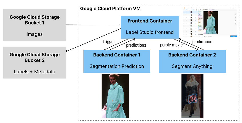
how to create your own backend with label studio, on top of the existing segment anything backend, for semiautomatic image segmentation labeling,
how to host on Google Cloud Platform for group collaboration, and
how to employ Google Cloud Storage buckets for data versioning.
Code in this post can be found in this GitHub repo.
Overview
Goal
Segment and identify the names and typologies of fashion clothing items in runway show images, as shown in the first image.
Why semiautomatic?
Wouldn’t it be nice if a trained segmentation model out there could perfectly recognize every piece of clothing in the runway show images? Sadly, there isn’t one. There exist trained models tailored to fashion or clothing images but nothing can match our dataset perfectly. Each fashion designer has their own style and preferences for certain clothing items and their color and texture, so even if a segmentation model can be 60% accurate, we call it a win. Then, we still need humans in the loop to correct what the segmentation model got wrong.
Entering Label Studio
Label Studio provides an open-source, customizable, and free-of-charge community version for various types of data labeling. One can create their own backend, so I can connect the Label Studio frontend to the trained segmentation model (mentioned above) backend for labelers to further improve upon the auto-predictions. Furthermore, Label Studio already has an interface that looks somewhat similar to Photoshop and a series of segmentation tools that can come in handy for us:
Segment Anything backend which harnesses the power of Meta’s SAM and allows you to recognize the object within a bounding box you draw.
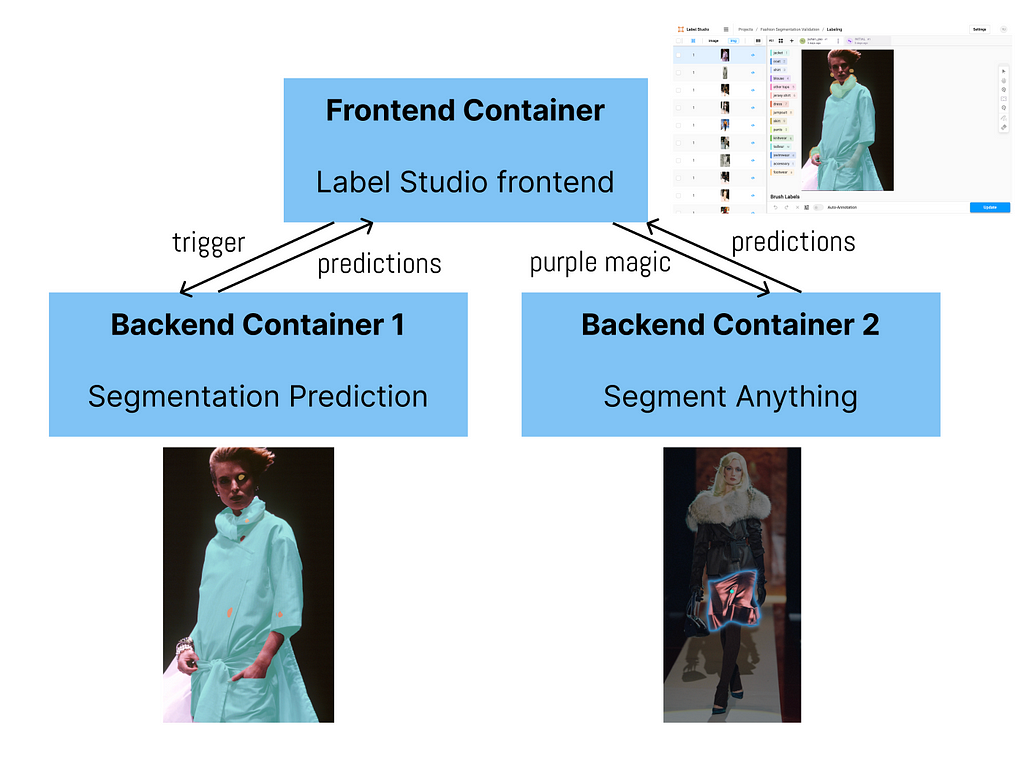
1 frontend + 2 backends
So far, we want 2 backends to be connected to the frontend. One backend can do the segmentation prediction and the second can speed up labelers’ modification if the predictions are wrong.
Image by Author
Implementation (Local)
Now, let’s fire up the app locally. That is, you will be able to use the app on your laptop or local machine completely for free but you are not able to invite your labeling team to collaborate on their laptops yet. We will talk about teamwork with GCP in the next section.
1. Install git and docker & download backend code
If you don’t have git or docker on your laptop or local machine yet, please install them. (Note: you can technically bypass the step of installing git if you download the zip file from this GitHub repo. If you do so, skip the following.)
Then, open up your terminal and clone this repo to a directory you want.
If you open up the label-studio-customized-ml-backend folder in your code editor, you can see the majority are adapted from the Label Studio ML backend repo, but this directory also contains frontend template code and SDK code adapted from Label Studio SDK.
2. Set up frontend to get access token
Following the official guidelines of segment anything, do the following in your terminal:
cd label-studio-customized-ml-backend/label_studio_ml/examples/segment_anything_model
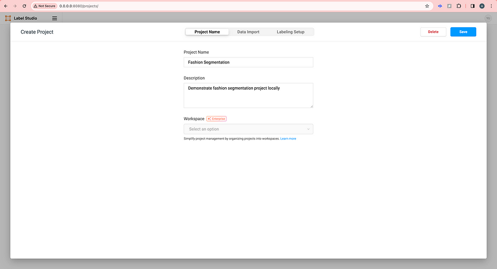
Then, open your browser and type http://0.0.0.0:8080/ and you will see the frontend of Label Studio. Proceed to sign up with your email address. Now, there is no project yet so we need to create our first project by clicking Create Project. Create a name and description (optional) for your project.
Image by Author
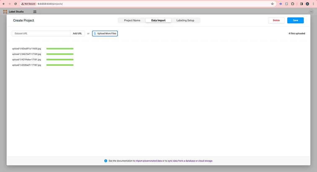
Upload some images locally. (We will talk about how to use cloud storage later.)
Image by Author
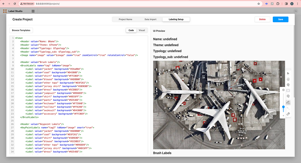
For Labeling Setup, click on Custom template on the left and copy-paste the HTML code from the label-studio-customized-ml-backend/label_studio_frontend/view.html file. You do not need the four lines of Headers if you don’t want to show image metadata in the labeling interface. Feel free to modify the code here to your need or click Visual to add or delete labels.
Image by Author
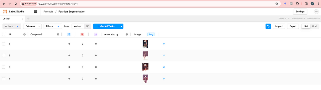
Now, click Save and your labeling interface should be ready.
Image by Author
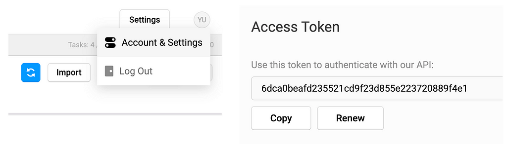
On the top right, click on the user setting icon and click Account & Setting and then you should be able to copy your access token.
Image by Author
3. Set up backend containers
In the label-studio-customized-ml-backend directory, there are many many backends thanks to the Label Studio developers. We will be using the customized ./segmentation backend for segmentation prediction (container 1) and the ./label_studio_ml/examples/segment_anything_model for faster labeling (container 2). The former will use port 7070 and the latter will use port 9090, making it easy to distinguish from the frontend port 8080.
Now, paste your access token to the 2 docker-compose.yml files in ./segmentationand ./label_studio_ml/examples/segment_anything_model folders.
Open up a new terminal and you cd into the segment_anything_model directory as you did before. Then, fire up the segment anything container.
cd label-studio-customized-ml-backend/label_studio_ml/examples/segment_anything_model

docker build . -t sam:latest
docker compose up
Then, open up another new terminal cd into the segmentation directory and fire up the segmentation prediction container.
cd label-studio-customized-ml-backend/segmentation

docker build . -t seg:latest
docker compose up
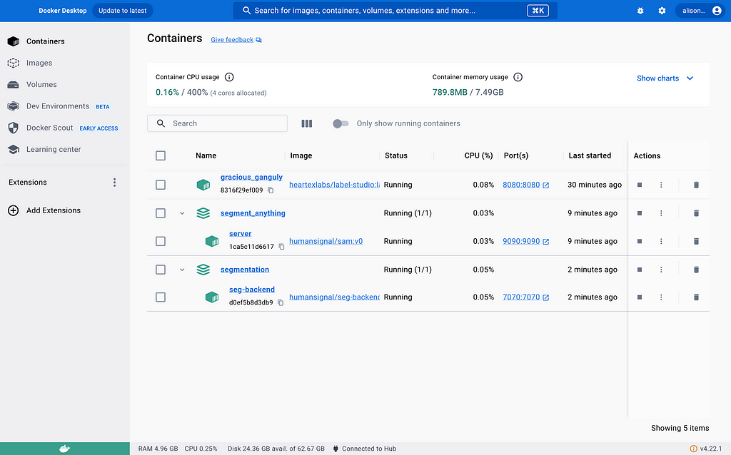
As of now, we have successfully started all 3 containers and you can double-check.
Image by Author
4. Connect containers
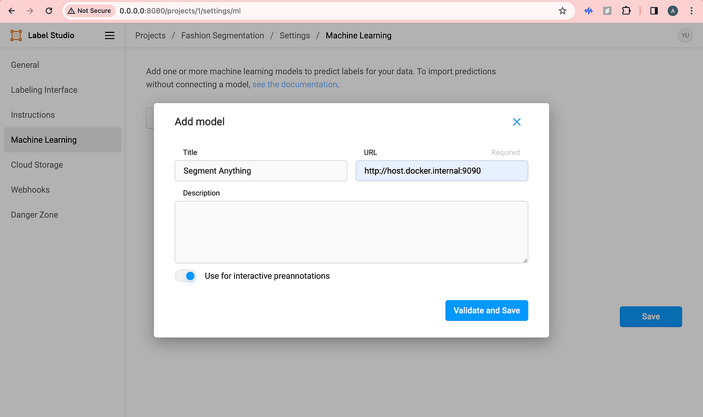
Before, what we did with the access token was helping us connect containers already, so we are almost done. Now, go to the frontend you started a while back and click Settings in the top right corner. Click Machine Learning on the left and click Add Model.
Image by Author
Be sure to use the URL with port 9090 and toggle on interactive preannotation. Finish adding by clicking Validate and Save.
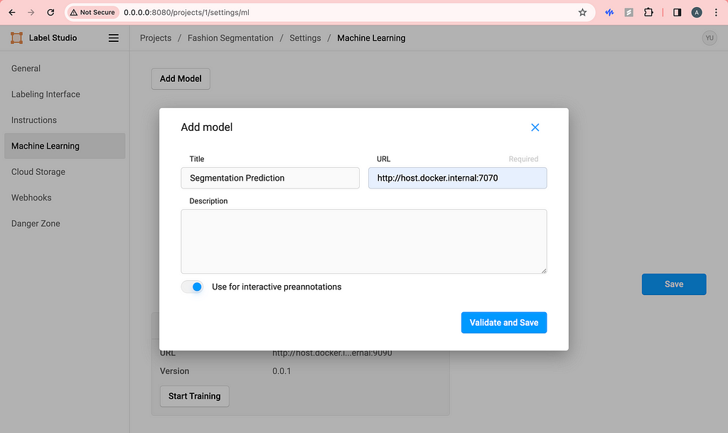
Similarly, do the same with the segmentation prediction backend.
Image by Author
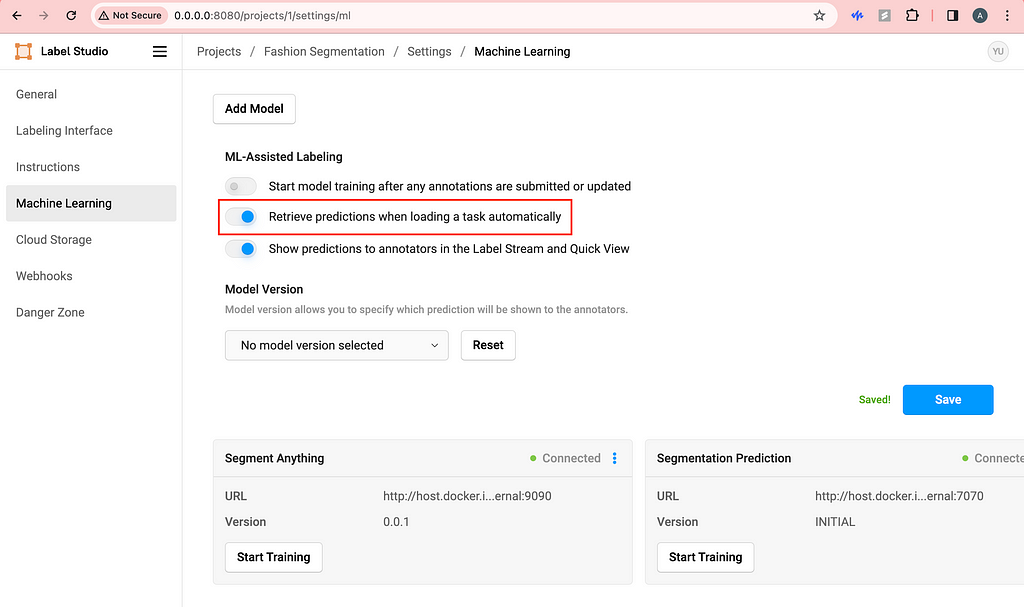
Then, I like to toggle on Retrieve predictions when loading a task automatically. This way, every time we refresh the labeling page, the segmentation predictions will be automatically triggered and loaded.
Image by Author
5. Happy labeling!
Here is a demo of what you should see if you follow the steps above.
If we are not happy with the predictions of let’s say the skirt, we can delete the skirt and use the purple magic (segment anything) to quickly label it.
I’m sure you can figure out how to use the brush, eraser and magic wand on your own!
If you are working solo, you are all set. But if you are wondering how to collaborate with your team without subscribing to Label Studio Enterprise, we need to host everything on cloud.
GCP Deployment
I chose GCP because of education credits, but you can use any cloud of your choice. The point is to host the app on cloud so that anyone in your labeling team can access and use your Label Studio app.
Image by Author
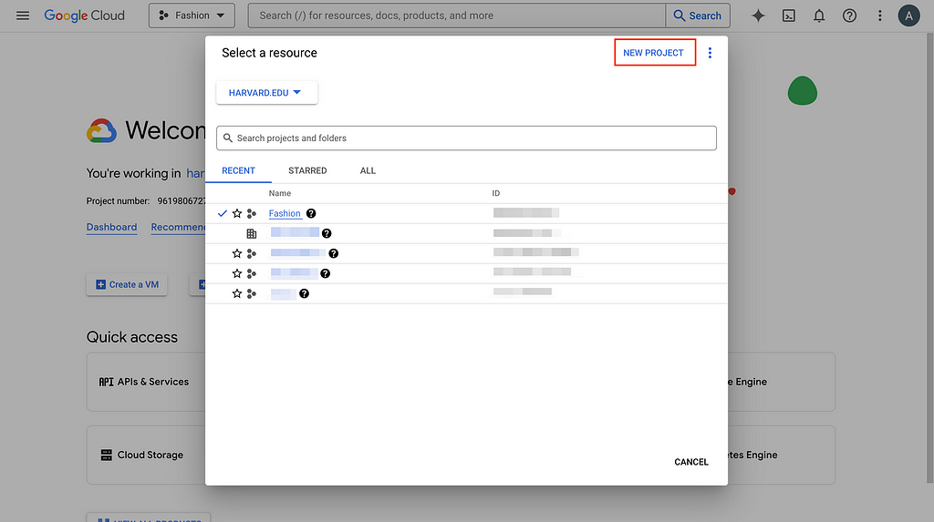
1. Select project/Create new project and set up billing account
Go to GCP console and create a new project if you don’t have an existing one and set up the billing account information as required (unfortunately, cloud costs some money). Here, I will use the Fashion project I created to demonstrate.
Image by Author
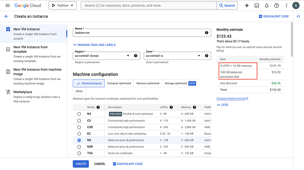
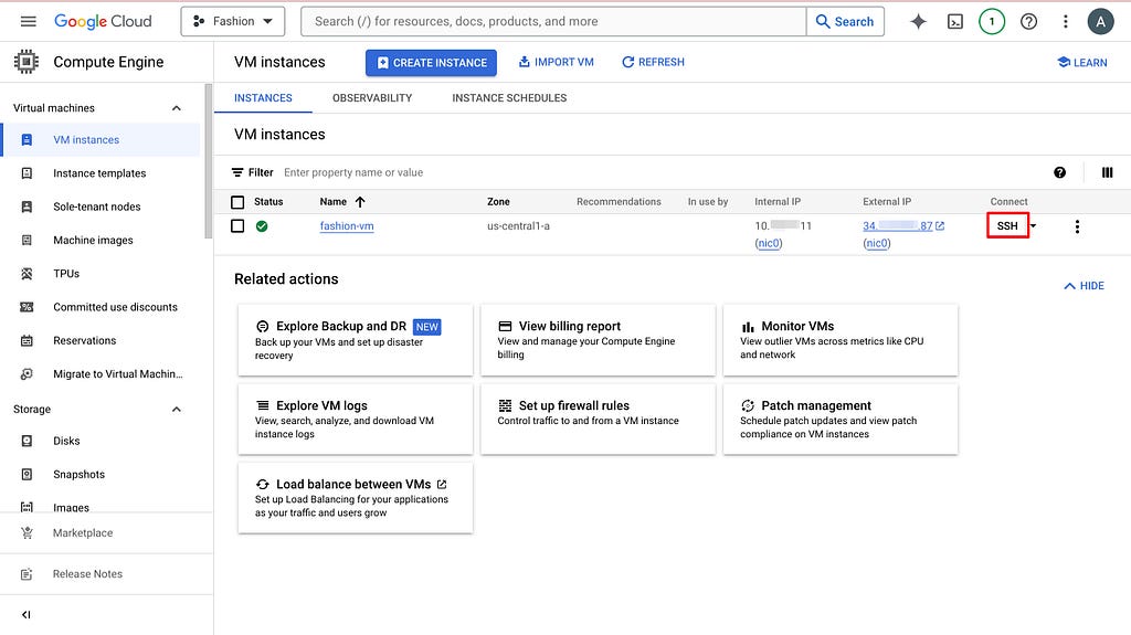
2. Create VM instance
To have a public IP address for labeling teamwork, we need to create a Virtual Machine (VM) on GCP and host everything here. After going to the project you created or selected, search compute engine in the search bar and the first thing that pops up should be VM instances. Click CREATE INSTANCE and choose the setting based on your need.
Image by Author
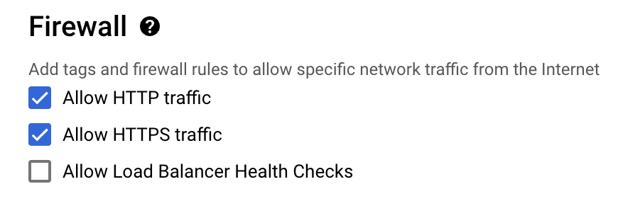
The default 10GB persistent disk will give you problems, so bump it up please. And more importantly, allow HTTP traffic.
Image by Author
It is a bit painful to modify these settings later, so try to think it through before clicking CREATE.
3. Set up VM environment
You can think of a VM as a computer somewhere in the cloud, similar to your laptop, but you can only ask it to do things via the terminal or command line. So now we need to set up everything on the VM the same way we set up everything locally (see previous section).
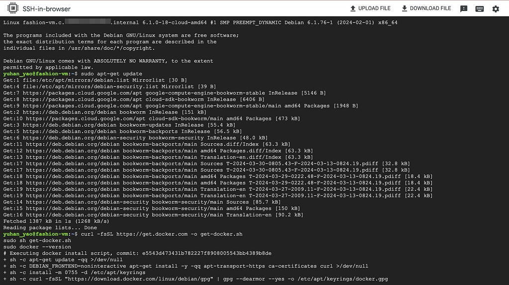
Click SSH, authorize and open up the command line interface.
Image by Author
Do routine update and install docker, docker compose, git and Python.
4. Follow previous section & set up everything on VM
Now, you can follow steps 1–4 in the previous section but there are some changes:
Add sudo when you have docker permission denied error.
If you have data permission error, modify permission using something like sudo chmod -R 777 mydata. And then you should be able to run your frontend container.
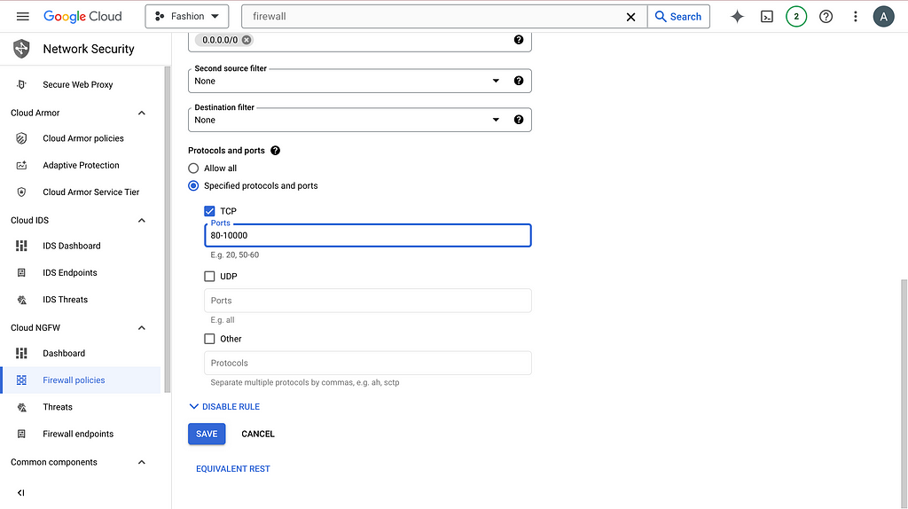
The server is not at http://0.0.0.0:8080 anymore. Instead, swap 0.0.0.0 with the external IP address of your VM. An example is http://34.1.1.87:8080/. You can find the external IP address next to the SSH button you clicked before. However, you probably still cannot access the frontend just yet. You need to search firewall on GCP console and click Firewall (VPC network) and then click default-allow-http. Now, change the setting to the following and you should be able to access the frontend.
Image by Author
4. When editing docker-compose.yml files, apart from copy-pasting access token, also modify the LABEL_STUDIO_HOST. Again, swap host.docker.internal with the VM external IP address. An example is http://34.1.1.87:8080 .
You can then export your labeling results and tailor to your uses.
If you only have a couple of images to label or you are fine with uploading images from local, by all means. But for my project, there are thousands of images, so I prefer using Google Cloud Storage to automate data transferring and data versioning.
GCS Integration
1. Set up GCS buckets
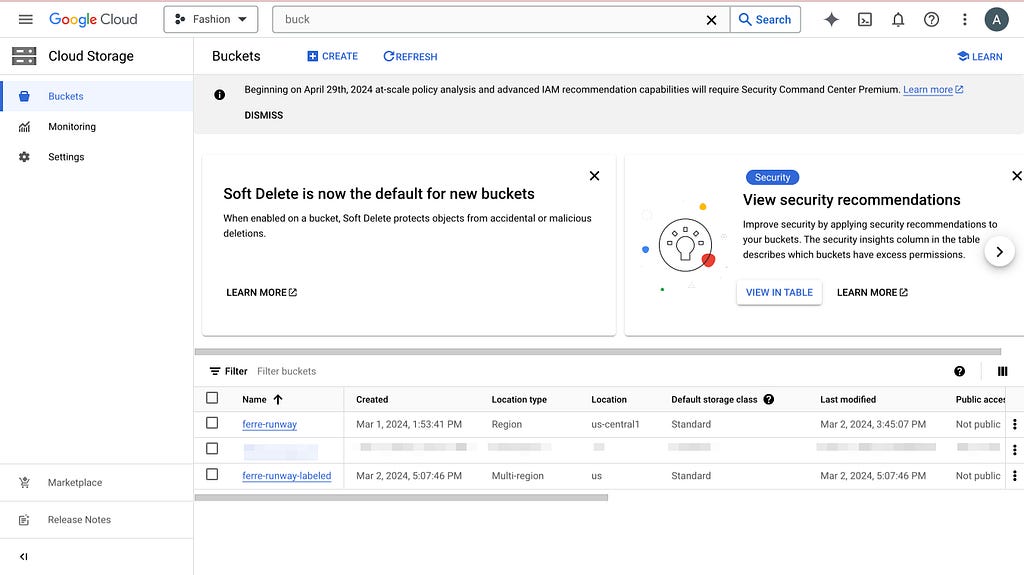
Search bucket in the GCP console and navigate to Cloud Storage buckets. Create 2 buckets: one with your images (source) and another empty (target). The second one will be populated later when you start labeling.
Image by Author
Then, following the official documentation, we need to set up cross-origin resource sharing (CORS) access to the buckets. Click Activate Cloud Shell on the top right, and run the following commands.
gsutil cors set cors-config.json gs://ferre-runway # use your bucket name gsutil cors set cors-config.json gs://ferre-runway-labeled # use your bucket name
If you want to set up data versioning for the labeling results, you can click on the bucket and turn on versioning in PROTECTION.
Image by Author
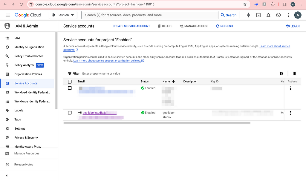
2. Create & set up service account key
Chances are that you do not want your buckets to be public, then label studio needs authentication to have access to these images. Click CREATE SERVICE ACCOUNT and grant the role of Storage Admin so that we can read and write to the GCS buckets. You should be able to see this service account in the permissions list of the buckets as well.
Image by Author
Now, click on the newly created service account and click KEYS. Now add a new key and be sure to download the JSON file to somewhere safe.
Now, open up your local terminal and encode the JSON file.
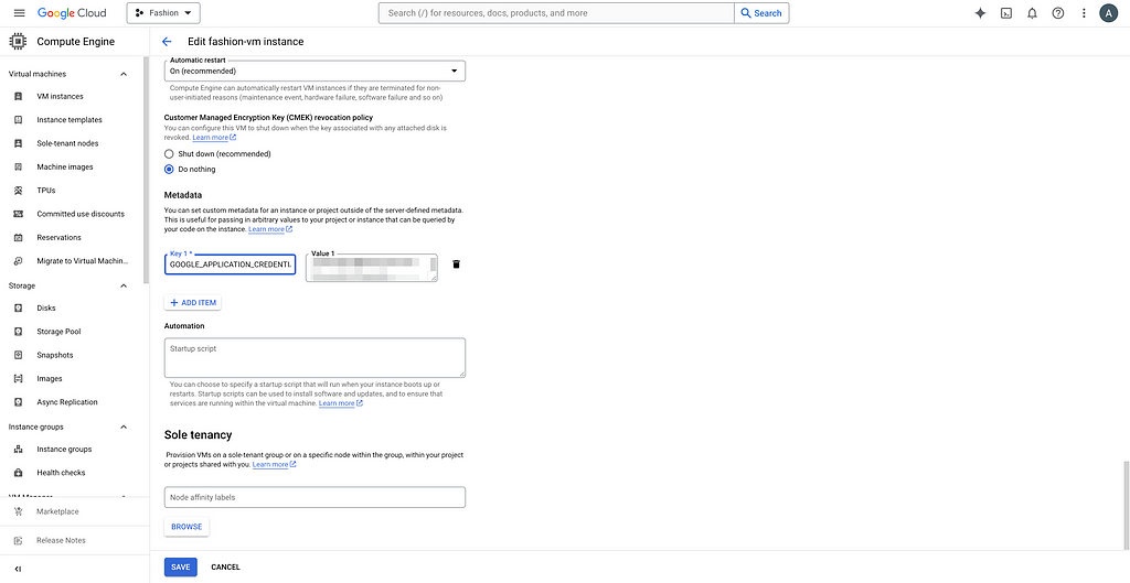
You can see the random character and number string and copy it. We are now pasting it as metadata for the VM. Click on your VM, click EDIT, and add your custom metadata. For example, my key is GOOGLE_APPLICATION_CREDENTIALS_BASE64.
Image by Author
We will then decode the service account key for authentication in our Python code.
3. Rebuild backend containers
Since we modified the docker-compose.yml files, we need to run the new script and rebuild the backend containers.
# Check running containers and their IDs, find the backends you need to kill sudo docker ps
# navigate to the right folders like before and build new containers sudo docker compose up
Now, you should see the new containers.
Image by Author
4. SDK upload images from source bucket
If you simply want to upload the images without metadata, you can skip this section and do the exact same thing as step 5 (see next). By metadata, I mean the useful information for each image on the labeling interface that might help with labeling more accurately.
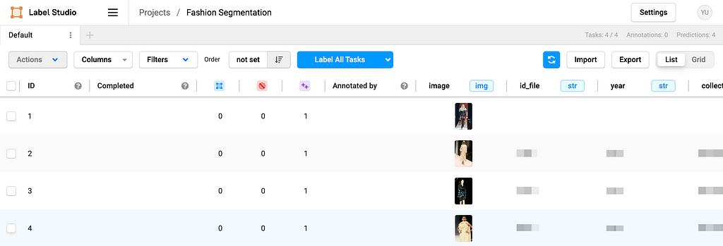
Based on the example from Label Studio SDK repo, you can modify what metadata and how you want to import in the ./label_studio_sdk/annotate_data_from_gcs.ipynb file. After running the python notebook locally, you should be able to see your images and metadata on the frontend.
Image by Author
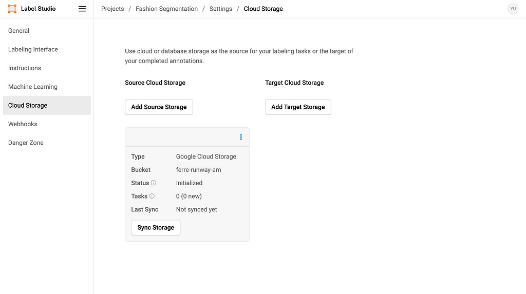
And you should also see the Source Storage bucket in the settings. Do NOT click Sync Storage as it will sync directly from the bucket and mess up the metadata we imported.
Image by Author
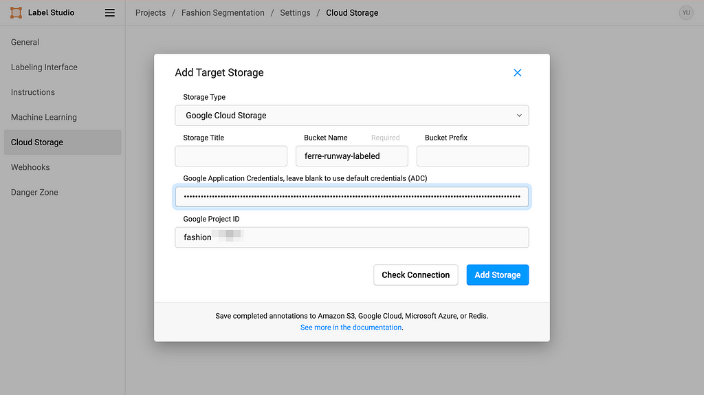
5. Set up Target Storage
Click Add Target Storage, and filling in the information accordingly. Copy-paste your service account key in the Google Application Credentials textbox and you are all set.
Image by Author
Every time you click Sync Storage on the Target Cloud Storage, it will sync the labeling outcome in the format of text into the GCS bucket. After clicking sync once, the process should be trigger automatically when submitting labeling results, but please check if you need to manually sync from time to time just in case.
Happy labeling!
Acknowledgement
It is my pleasure to be a part of Data Shack 2024 in collaboration with Politecnico de Milano Gianfranco Ferré Research Center. I would like to thank Prof. Pavlos Protopapas and Prof. Paola Bertola for your guidance and for making this project happen in the first place. I would like to thank Chris Gumb and Prof. Marco Brambilla for technical support and Prof. Federica Vacca and Dr. Angelica Vandi for domain knowledge expertise in fashion. Finally, I would like to thank my teammates Luis Henrique Simplicio Ribeiro, Lorenzo Campana and Vittoria Corvetti for your help and for figuring things out with me along the way. I also want to give a round of applause to Emanuela Di Stefano, Jacopo Sileo, Bruna Pio Da Silva Rigato, Martino Fois, Xinxi Liu, and Ilaria Trame for your continued support and hard work.
References
11655 Gianfranco Ferré, Ready-To-Wear Collection, Fall-Winter 2004. Courtesy of Gianfranco Ferré Research Center
13215 Gianfranco Ferré, Ready-To-Wear Collection, Spring-Summer 1991. Courtesy of Gianfranco Ferré Research Center
Thank you for reading! I hope this blog has been helpful to you.
Code in this post can be found in this GitHub repo.
We use cookies on our website to give you the most relevant experience by remembering your preferences and repeat visits. By clicking “Accept”, you consent to the use of ALL the cookies.
This website uses cookies to improve your experience while you navigate through the website. Out of these, the cookies that are categorized as necessary are stored on your browser as they are essential for the working of basic functionalities of the website. We also use third-party cookies that help us analyze and understand how you use this website. These cookies will be stored in your browser only with your consent. You also have the option to opt-out of these cookies. But opting out of some of these cookies may affect your browsing experience.
Necessary cookies are absolutely essential for the website to function properly. These cookies ensure basic functionalities and security features of the website, anonymously.
Cookie
Duration
Description
cookielawinfo-checkbox-analytics
11 months
This cookie is set by GDPR Cookie Consent plugin. The cookie is used to store the user consent for the cookies in the category "Analytics".
cookielawinfo-checkbox-functional
11 months
The cookie is set by GDPR cookie consent to record the user consent for the cookies in the category "Functional".
cookielawinfo-checkbox-necessary
11 months
This cookie is set by GDPR Cookie Consent plugin. The cookies is used to store the user consent for the cookies in the category "Necessary".
cookielawinfo-checkbox-others
11 months
This cookie is set by GDPR Cookie Consent plugin. The cookie is used to store the user consent for the cookies in the category "Other.
cookielawinfo-checkbox-performance
11 months
This cookie is set by GDPR Cookie Consent plugin. The cookie is used to store the user consent for the cookies in the category "Performance".
viewed_cookie_policy
11 months
The cookie is set by the GDPR Cookie Consent plugin and is used to store whether or not user has consented to the use of cookies. It does not store any personal data.
Functional cookies help to perform certain functionalities like sharing the content of the website on social media platforms, collect feedbacks, and other third-party features.
Performance cookies are used to understand and analyze the key performance indexes of the website which helps in delivering a better user experience for the visitors.
Analytical cookies are used to understand how visitors interact with the website. These cookies help provide information on metrics the number of visitors, bounce rate, traffic source, etc.
Advertisement cookies are used to provide visitors with relevant ads and marketing campaigns. These cookies track visitors across websites and collect information to provide customized ads.