Tag: AI

How to calculate probability when “we absolutely know nothing antecedently to any trials made” (Bayes, 1763)

Contents

1. Introduction
2. Priors and Frequentist Matching
   – example 1: a normal distribution with unknown mean
   – example 2: a normal distribution with unknown variance
3. The Binomial Distribution Prior
4. Applications from Bayes and Laplace
   – example 3: observing only 1s
   – example 4: a lottery
   – example 5: birth rates
5. Discussion
6. Conclusion
7. Notes and References

Introduction

In 1654 Pascal and Fermat worked together to solve the problem of the points [1] and in so doing developed an early theory for deductive reasoning with direct probabilities. Thirty years later, Jacob Bernoulli worked to extend probability theory to solve inductive problems. He recognized that unlike in games of chance, it was futile to a priori enumerate possible cases and find out “how much more easily can some occur than the others”:

But, who from among the mortals will be able to determine, for example, the number of diseases, that is, the same number of cases which at each age invade the innumerable parts of the human body and can bring about our death; and how much easier one disease (for example, the plague) can kill a man than another one (for example, rabies; or, the rabies than fever), so that we would be able to conjecture about the future state of life or death? And who will count the innumerable cases of changes to which the air is subjected each day so as to form a conjecture about its state in a month, to say nothing about a year? Again, who knows the nature of the human mind or the admirable fabric of our body shrewdly enough for daring to determine the cases in which one or another participant can gain victory or be ruined in games completely or partly depending on acumen or agility of body? [2, p. 18]

The way forward, he reasoned, was to determine probabilities a posteriori

Here, however, another way for attaining the desired is really opening for us. And, what we are not given to derive a priori, we at least can obtain a posteriori, that is, can extract it from a repeated observation of the results of similar examples. [2, p. 18]

To establish the validity of the approach, Bernoulli proved a version of the law of large numbers for the binomial distribution. Let X_n represent a sample from a Bernoulli distribution with parameter r/t (r and t integers). Then if c represents some positive integer, Bernoulli showed that for N large enough

In other words, the probability the sampled ratio from a binomial distribution is contained within the bounds (r−1)/t to (r+1)/t is at least c times more likely than the the probability it is outside the bounds. Thus, by taking enough samples, “we determine the [parameter] a posteriori almost as though it was known to us a prior”.

Bernoulli, additionally, derived lower bounds, given r and t, for how many samples would be needed to achieve a desired levels of accuracy. For example, if r = 30 and t = 50, he showed

having made 25550 experiments, it will be more than a thousand times more likely that the ratio of the number of obtained fertile observations to their total number is contained within the limits 31/50 and 29/50 rather than beyond them [2, p. 30]

This suggested an approach to inference, but it came up short in several respects. 1) The bounds derived were conditional on knowledge of the true parameter. It didn’t provide a way to quantify uncertainty when the parameter was unknown. And 2) the number of experiments required to reach a high level of confidence in an estimate, moral certainty in Bernoulli’s words, was quite large, limiting the approach’s practicality. Abraham de Moivre would later improve on Bernoulli’s work in his highly popular textbook The Doctrine of Chances. He derived considerably tighter bounds, but again failed to provide a way to quantify uncertainty when the binomial distribution’s parameter was unknown, offering only this qualitative guidance:

if after taking a great number of Experiments, it should be perceived that the happenings and failings have been nearly in a certain proportion, such as of 2 to 1, it may safely be concluded that the Probabilities of happening or failing at any one time assigned will be very near that proportion, and that the greater the number of Experiments has been, so much nearer the Truth will the conjectures be that are derived from them. [3, p. 242]

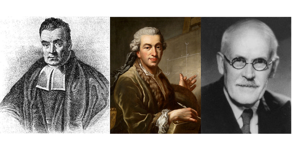
Inspired by de Moivre’s book, Thomas Bayes took up the problem of inference with the binomial distribution. He reframed the goal to

Given the number of times in which an unknown event has happened and failed: Required the chance that the probability of its happening in a single trial lies somewhere between any two degrees of probability that can be named. [4, p. 4]

Recognizing that a solution would depend on prior probability, Bayes sought to give an answer for

the case of an event concerning the probability of which we absolutely know nothing antecedently to any trials made concerning it [4, p. 11]

He reasoned that knowing nothing was equivalent to a uniform prior distribution [5, p. 184–188]. Using the uniform prior and a geometric analogy with balls, Bayes succeeded in approximating integrals of posterior distributions of the form

and was able to answer questions like “If I observe y success and n − y failures from a binomial distribution with unknown parameter θ, what is the probability that θ is between a and b?”.

Despite Bayes’ success answering inferential questions, his method was not widely adopted and his work, published posthumously in 1763, remained obscure up until De Morgan renewed attention to it over fifty years later. A major obstacle was Bayes’ presentation; as mathematical historian Stephen Stigler writes,

Bayes essay ’Towards solving a problem in the doctrine of chances’ is extremely difficult to read today–even when we know what to look for. [5, p. 179]

A decade after Bayes’ death and likely unaware of his discoveries, Laplace pursued similar problems and independently arrive at the same approach. Laplace revisited the famous problem of the points, but this time considered the case of a skilled game where the probability of a player winning a round was modeled by a Bernoulli distribution with unknown parameter p. Like Bayes, Laplace assumed a uniform prior, noting only

because the probability that A will win a point is unknown, we may suppose it to be any unspecified number whatever between 0 and 1. [6]

Unlike Bayes, though, Laplace did not use a geometric approach. He approached the problems with a much more developed analytical toolbox and was able to derive more usable formulas with integrals and clearer notation.

Following Laplace and up until the early 20th century, using a uniform prior together with Bayes’ theorem became a popular approach to statistical inference. In 1837, De Morgan introduced the term inverse probability to refer to such methods and acknowledged Bayes’ earlier work:

De Moivre, nevertheless, did not discover the inverse method. This was first used by the Rev. T. Bayes, in Phil. Trans. liii. 370.; and the author, though now almost forgotten, deserves the most honourable rememberance from all who read the history of this science. [7, p. vii]

In the early 20th century, inverse probability came under serious attack for its use of a uniform prior. Ronald Fisher, one of the fiercest critics, wrote

I know only one case in mathematics of a doctrine which has been accepted and developed by the most eminent men of their time, and is now perhaps accepted by men now living, which at the same time has appeared to a succession of sound writers to be fundamentally false and devoid of foundation. Yet that is quite exactly the position in respect of inverse probability [8]

Note: Fisher was not the first to criticize inverse probability, and he references the earlier works of Boole, Venn, and Chrystal. See [25] for a detailed account of inverse probability criticism leading up to Fisher.

Fisher criticized inverse probability as “extremely arbitrary”. Reviewing Bayes’ essay, he pointed out how naive use of a uniform prior leads to solutions that depend on the scale used to measure probability. He gave a concrete example [9]: Let p denote the unknown parameter for a binomial distribution. Suppose that instead of p we parameterize by

and apply the uniform prior. Then the probability that θ is between a and b after observing S successes and F failures is

A change of variables back to p shows us this is equivalent to

Hence, the uniform prior in θ is equivalent to the prior 1/π p^{−1/2} (1 − p)^{−1/2} in p. As an alternative to inverse probability, Fisher promoted maximum likelihood methods, p-values, and a frequentist definition for probability.

While Fisher and others advocated for abandoning inverse probability in favor of frequentist methods, Harold Jeffreys worked to put inverse probability on a firmer foundation. He acknowledged earlier approaches had lacked consistency, but he agreed with their goal of delivering statistical results in terms of degree of belief and thought frequentist definitions of probability to be hopelessly flawed:

frequentist definitions themselves lead to no results of the kind that we need until the notion of reasonable degree of belief is reintroduced, and that since the whole purpose of these definitions is to avoid this notion they necessarily fail in their object. [10, p. 34]

Jeffreys pointed out that inverse probability needn’t be tied to the uniform prior:

There is no more need for [the idea that the uniform distribution of
the prior probability was a necessary part of the principle of inverse probability] than there is to say that an oven that has once cooked roast beef can never cook anything but roast beef. [10, p. 103]

Seeking to achieve results that would be consistent under reparameterization, Jeffreys proposed priors based on the Fisher information matrix,

writing,

If we took the prior probability density for the parameters to be proportional to [(det I(θ))^{1/2}] … any arbitrariness in the choice of the parameters could make no difference to the results, and it is proved that for this wide class of laws a consistent theory of probability can be constructed. [10, p. 159]

Note: If Θ denotes a region of the parameter space and φ(u) is an injective continuous function whose range includes Θ, then applying the change-of-variables formula will show that

where I^φ denotes the Fisher information matrix with respect to the reparameterization, φ.

Twenty years later, Welch and Peers investigated priors from a different perspective [11]. They analyzed one-tailed credible sets from posterior distributions and asked how closely probability mass coverage matched frequentist coverage. They found that for the case of a single parameter, the prior Jeffreys proposed was asymptotically optimal, providing further justification for the prior that aligned with how intuition suggests we might quantify Bayes criterion of “knowing absolutely nothing”.

Note: Deriving good priors in the multi-parameter case is considerably more involved. Jeffreys himself was dissatisfied with the priors his rule produced for multi-parameter models and proposed an alternative known as Jeffreys independent prior but never developed a rigorous approach. José-Miguel Bernardo and James Berger would later develop reference priors as a refinement of Jeffreys prior. Reference priors provide a general mechanism to produce good priors that works for multi-parameter models and cases where the Fisher information matrix doesn’t exist. See [13] and [14, part 3].

In an unfortunate turn of events, mainstream statistics mostly ignored Jeffreys approach to inverse probability to chase a mirage of objectivity that frequentist methods seemed to provide.

Note: Development of inverse probability in the direction Jeffreys outlined continued under the name objective Bayesian analysis; however, it hardly occupies the center stage of statistics, and many people mistakenly think of Bayesian analysis as more of a subjective theory.

See [21] for background on why the objectivity that many perceive frequentist methods to have is largely false.

But much as Jeffreys had anticipated with his criticism that frequentist definitions of probability couldn’t provide “results of the kind that we need”, a majority of practitioners filled in the blank by misinterpreting frequentist results as providing belief probabilities. Goodman coined the term P value fallacy to refer to this common error and described just how prevalent it is

In my experience teaching many academic physicians, when physicians are presented with a single-sentence summary of a study that produced a surprising result with P = 0.05, the overwhelming majority will confidently state that there is a 95% or greater chance that the null hypothesis is incorrect. [12]

James Berger and Thomas Sellke established theoretical and simulation results that show how spectacularly wrong this notion is

it is shown that actual evidence against a null (as measured, say, by posterior probability or comparative likelihood) can differ by an order of magnitude from the P value. For instance, data that yield a P value of .05, when testing a normal mean, result in a posterior probability of the null of at least .30 for any objective prior distribution. [15]

They concluded

for testing “precise” hypotheses, p values should not be used directly, because they are too easily misinterpreted. The standard approach in teaching–of stressing the formal definition of a p value while warning against its misinterpretation–has simply been an abysmal failure. [16]

In this post, we’ll look closer at how priors for objective Bayesian analysis can be justified by matching coverage; and we’ll reexamine the problems Bayes and Laplace studied to see how they might be approached with a more modern methodology.

Priors and Frequentist Matching

The idea of matching priors intuitively aligns with how we might think about probability in the absence of prior knowledge. We can think of the frequentist coverage matching metric as a way to provide an answer to the question “How accurate are the Bayesian credible sets produced with a given prior?”.

Note: For more background on frequentist coverage matching and its relation to objective Bayesian analysis, see [17] and [14, ch. 5].

Consider a probability model with a single parameter θ. If we’re given a prior, π(θ), how do we test if the prior reasonably expresses Bayes’ requirement of knowing nothing? Let’s pick a size n, a value θ_true, and randomly sample observations y = (y1, . . ., yn)^T from the distribution P( · |θ_true). Then let’s compute the two-tailed credible set [θ_a, θ_b] that contains 95% of the probability mass of the posterior,

and record whether or not the credible set contains θ_true. Now suppose we repeat the experiment many times and vary n and θ_true. If π(θ) is a good prior, then the fraction of trials where θ_true is contained within the credible set will consistently be close to 95%.

Here’s how we might express this experiment as an algorithm:

function coverage-test(n, θ_true, α):
  cnt ← 0
  N ← a large number
  for i ← 1 to N do
    y ← sample from P(·|θ_true)
    t ← integrate_{-∞}^θ_true π(θ | y)dθ
    if (1 - α)/2 < t < 1 - (1 - α)/2:
      cnt ← cnt + 1
    end if
  end for
  return cnt / N

Example 1: a normal distribution with unknown mean

Suppose we observe n normally distributed values, y, with variance 1 and unknown mean, μ. Let’s consider the prior

Note: In this case Jeffreys prior and the constant prior in μ are the same.

Then

Thus,

I ran a 95% coverage test with 10000 trials and various values of μ and n. As the table below shows, the results are all close to 95%, indicating the constant prior is a good choice in this case. [Source code for example].

Example 2: a normal distribution with unknown variance

Now suppose we observe n normally distributed values, y, with unknown variance and zero mean, μ. Let’s test the constant prior and Jeffreys prior,

We have

where s²=y’y/n. Put u=ns²/(2σ²). Then

Thus,

Similarly,

The table below shows the results for a 95% coverage test with the constant prior. We can see that coverage is notably less than 95% for smaller values of n.

In comparison, coverage is consistently close to 95% for all values of n if we use Jeffreys prior. [Source code for example].

The Binomial Distribution Prior

Let’s apply Jeffreys approach to inverse probability to the binomial distribution.

Suppose we observe n values from the binomial distribution. Let y denote the number of successes and θ denote the probability of success. The likelihood function is given by

Taking the log and differentiating, we have

Thus, the Fisher information matrix for the binomial distribution is

and Jeffreys prior is

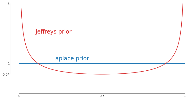
The posterior is then

which we can recognize as the beta distribution with parameters y+1/2 and n-y+1/2.

To test frequentist coverages, we can use an exact algorithm.

function binomial-coverage-test(n, θ_true, α):
  cov ← 0
  for y ← 0 to n do
    t ← integrate_0^θ_true π(θ | y)dθ
    if (1 - α)/2 < t < 1 - (1 - α)/2:
      cov ← cov + binomial_coefficient(n, y) * θ_true^y * (1 - θ_true)^(n-y)
    end if
  end for
  return cov

Here are the coverage results for α=0.95 and various values of p and n using the Bayes-Laplace uniform prior:

and here are the coverage results using Jeffreys prior:

We can see coverage is identical for many table entries. For smaller values of n and p_true, though, the uniform prior gives no coverage while Jeffreys prior provides decent results. [source code for experiment]

Applications from Bayes and Laplace

Let’s now revisit some applications Bayes and Laplace studied. Given that the goal in all of these problems is to assign a belief probability to an interval of the parameter space, I think that we can make a strong argument that Jeffreys prior is a better choice than the uniform prior since it has asymptotically optimal frequentist coverage performance. This also addresses Fisher’s criticism of arbitrariness.

Note: See [14, p. 105–106] for a more through discussion of the uniform prior vs Jeffreys prior for the binomial distribution

In each of these problems, I’ll show both the answer given by Jeffreys prior and the original uniform prior that Bayes and Laplace used. One theme we’ll see is that many of the results are not that different. A lot of fuss is often made over minor differences in how objective priors can be derived. The differences can be important, but often the data dominates and different reasonable choices will lead to nearly the same result.

Example 3: Observing Only 1s

In an appendix Richard Price added to Bayes’ essay, he considers the following problem:

Let us then first suppose, of such an event as that called M in the essay, or an event about the probability of which, antecedently to trials, we know nothing, that it has happened once, and that it is enquired what conclusion we may draw from hence with respct to the probability of it’s happening on a second trial. [4, p. 16]

Specifically, Price asks, “what’s the probability that θ is greater than 1/2?” Using the uniform prior in Bayes’ essay, we derive the posterior distribution

Integrating gives us the answer

Using Jeffreys prior, we derive a beta distribution for the posterior

and the answer

Price then continues with the same problem but supposes we see two 1s, three 1s, etc. The table below shows the result we’d get up to ten 1s. [source code]

Example 4: A Lottery

Price also considers a lottery with an unknown chance of winning:

Let us then imagine a person present at the drawing of a lottery, who knows nothing of its scheme or of the proportion of Blanks to Prizes in it. Let it further be supposed, that he is obliged to infer this from the number of blanks he hears drawn compared with the number of prizes; and that it is enquired what conclusions in these circumstances he may reasonably make. [4, p. 19–20]

He asks this specific question:

Let him first hear ten blanks drawn and one prize, and let it be enquired what chance he will have for being right if he gussses that the proportion of blanks to prizes in the lottery lies somewhere between the proportions of 9 to 1 and 11 to 1. [4, p. 20]

With Bayes prior and θ representing the probability of drawing a blank, we derive the posterior distribution

and the answer

Using Jeffreys prior, we get the posterior

and the answer

Price then considers the same question (what’s the probability that θ lies between 9/10 and 11/12) for different cases where an observer of the lottery sees w prizes and 10w blanks. Below I show posterior probabilities using both Bayes’ uniform prior and Jeffreys prior for various values of w. [source code]

Example 5: Birth Rates

Let’s now turn to a problem that fascinated Laplace and his contemporaries: The relative birth rate of boys-to-girls. Laplace introduces the problem,

The consideration of the [influence of past events on the probability of future events] leads me to speak of births: as this matter is one of the most interesting in which we are able to apply the Calculus of probabilities, I manage so to treat with all care owing to its importance, by determining what is, in this case, the influence of the observed events on those which must take place, and how, by its multiplying, they uncover for us the true ratio of the possibilities of the births of a boy and of a girl. [18, p. 1]

Like Bayes, Laplace approaches the problem using a uniform prior, writing

When we have nothing given a priori on the possibility of an event, it is necessary to assume all the possibilities, from zero to unity, equally probable; thus, observation can alone instruct us on the ratio of the births of boys and of girls, we must, considering the thing only in itself and setting aside the events, to assume the law of possibility of the births of a boy or of a girl constant from zero to unity, and to start from this hypothesis into the different problems that we can propose on this object. [18, p. 26]

Using data collection from Paris between 1745 and 1770, where 251527 boys and 241945 girls had been born, Laplace asks, what is “the probability that the possibility of the birth of a boy is equal or less than 1/2“?

With a uniform prior, B = 251527, G = 241945, and θ representing the probability that a boy is born, we obtain the posterior

and the answer

With Jeffreys prior, we similarly derive the posterior

and the answer

Here’s some simulated data using p_true = B / (B + G) that shows how the answers might evolve as more births are observed.

Discussion

Q1: Where does objective Bayesian analysis belong in statistics?

I think Jeffreys was right and standard statistical procedures should deliver “results of the kind we need”. While Bayes and Laplace might not have been fully justified in their choice of a uniform prior, they were correct in their objective of quantifying results in terms of degree of belief. The approach Jeffreys outlined (and was later evolved with reference priors) gives us a pathway to provide “results of the kind we need” while addressing the arbitrariness of a uniform prior. Jeffreys approach isn’t the only way to get to results as degrees of belief, and a more subjective approach can also be valid if the situation allows, but his approach give us good answers for the common case “of an event concerning the probability of which we absolutely know nothing” and can be used as a drop-in replacement for frequentist methods.

To answer more concretely, I think when you open up a standard introduction-to-statistics textbook and look up a basic procedure such as a hypothesis test of whether the mean of normally distributed data with unknown variance is non-zero, you should see a method built on objective priors and Bayes factor like [19] rather than a method based on P values.

Q2: But aren’t there multiple ways of deriving good priors in the absence of prior knowledge?

I highlighted frequentist coverage matching as a benchmark to gauge whether a prior is a good candidate for objective analysis, but coverage matching isn’t the only valid metric we could use and it may be possible to derive multiple priors with good coverage. Different priors with good frequentist properties, though, will likely be similar, and any results will be determined more by observations than the prior. If we are in a situation where multiple good priors lead to significantly differing results, then that’s an indicator we need to provide subjective input to get a useful answer. Here’s how Berger addresses this issue:

Inventing a new criterion for finding “the optimal objective prior” has proven to be a popular research pastime, and the result is that many competing priors are now available for many situations. This multiplicity can be bewildering to the casual user.

I have found the reference prior approach to be the most successful approach, sometimes complemented by invariance considerations as well as study of frequentist properties of resulting procedures. Through such considerations, a particular prior usually emerges as the clear winner in many scenarios, and can be put forth as the recommended objective prior for the situation. [20]

Q3. Doesn’t that make inverse probability subjective, whereas frequentist methods provide an objective approach to statistics?

It’s a common misconception that frequentist methods are objective. Berger and Berry provides this example to demonstrate [21]: Suppose we watch a research study a coin for bias. We see the researcher flip the coin 17 times. Heads comes up 13 times and tails comes up 4 times. Suppose θ represents the probability of heads and the researcher is doing a standard P-value test with the null hypothesis that the coin is not bias, θ=0.5. What P-value would they get? We can’t answer the question because the researcher would get remarkably different results depending on their experimental intentions.

If the researcher intended to flip the coin 17 times, then the probability of seeing a value less extreme than 13 heads under the null hypothesis is given by summing binomial distribution terms representing the probabilities of getting 5 to 12 heads,

which gives us a P-value of 1–0.951=0.049.

If, however, the researcher intended to continue flipping until they got at least 4 heads and 4 tails, then the probability of seeing a value less extreme than 17 total flips under the null hypothesis is given by summing negative binomial distribution terms representing the probabilities of getting 8 to 16 total flips,

which gives us a P-value of 1–0.979=0.021

The result is dependent on not just the data but also on the hidden intentions of the researcher. As Berger and Berry argue “objectivity is not generally possible in statistics and … standard statistical methods can produce misleading inferences.” [21] [source code for example]

Q4. If subjectivity is unavoidable, why not just use subjective priors?

When subjective input is possible, we should incorporate it. But we should also acknowledge that Bayes’ “event concerning the probability of which we absolutely know nothing” is an important fundamental problem of inference that needs good solutions. As Edwin Jaynes writes

To reject the question, [how do we find the prior representing “complete ignorance”?], as some have done, on the grounds that the state of complete ignorance does not “exist” would be just as absurd as to reject Euclidean geometry on the grounds that a physical point does not exist. In the study of inductive inference, the notion of complete ignorance intrudes itself into the theory just as naturally and inevitably as the concept of zero in arithmetic.

If one rejects the consideration of complete ignorance on the grounds that the notion is vague and ill-defined, the reply is that the notion cannot be evaded in any full theory of inference. So if it is still ill-defined, then a major and immediate objective must be to find a precise definition which will agree with intuitive requirements and be of constructive use in a mathematical theory. [22]

Moreover, systematic approaches such as reference priors can certainly do much better than pseudo-Bayesian techniques such as choosing a uniform prior over a truncated parameter space or a vague proper prior such as a Gaussian over a region of the parameter space that looks interesting. Even when subjective information is available, using reference priors as building blocks is often the best way to incorporate it. For instance, if we know that a parameter is restricted to a certain range but don’t know anything more, we can simply adapt a reference prior by restricting and renormalizing it [14, p. 256].

Note: The term pseudo-Bayesian comes from [20]. See that paper for a more through discussion and comparison with objective Bayesian analysis.

Conclusion

The common and repeated misinterpretation of statistical results such as P values or confidence intervals as belief probabilities shows us that there is a strong natural tendency to want to think about inference in terms of inverse probability. It’s no wonder that the method dominated for 150 years.

Fisher and others were certainly correct to criticize naive use of a uniform prior as arbitrary, but this is largely addressed by reference priors and adopting metrics like frequentist matching coverage that quantify what it means for a prior to represent ignorance. As Berger puts it,

We would argue that noninformative prior Bayesian analysis is the single most powerful method of statistical analysis, in the sense of being the ad hoc method most likely to yield a sensible answer for a given investment of effort. And the answers so obtained have the added feature of being, in some sense, the most “objective” statistical answers obtainable [23, p. 90]

Notes & References

[1]: Problem of the points: Suppose two players A and B each contribute an equal amount of money into a prize pot. A and B then agree to play repeated rounds of a game of chance, with the players having an equal probability of winning any round, until one of the players has won k rounds. The player that first reaches k wins takes the entirety of the prize pot. Now, suppose the game is interrupted with neither player reaching k wins. If A has w_A wins and B has w_B wins, what’s a fair way to split the pot?

[2]: Bernoulli, J. (1713). On the Law of Large Numbers, Part Four of Ars Conjectandi. Translated by Oscar Sheynin.

[3]: De Moivre, A. (1756). The Doctrine of Chances.

[4]: Bayes, T. (1763). An essay towards solving a problem in the doctrine of chances. by the late rev. mr. bayes, f. r. s. communicated by mr. price, in a letter to john canton, a. m. f. r. s. Philosophical Transactions of the Royal Society of London 53, 370–418.

[5]: Stigler, S. (1990). The History of Statistics: The Measurement of Uncer- tainty before 1900. Belknap Press.

[6]: Laplace, P. (1774). Memoir on the probability of the causes of events. Translated by S. M. Stigler.

[7]: De Morgan, A. (1838). An Essay On Probabilities: And On Their Application To Life Contingencies And Insurance Offices.

[8]: Fisher, R. (1930). Inverse probability. Mathematical Proceedings of the Cambridge Philosophical Society 26(4), 528–535.

[9]: Fisher, R. (1922). On the mathematical foundations of theoretical statistics. Philosophical Transactions of the Royal Society of London. Series A, Containing Papers of a Mathematical or Physical Character 222, 309–368.

[10]: Jeffreys, H. (1961). Theory of Probability (3 ed.). Oxford Classic Texts in the Physical Sciences.

[11]: Welch, B. L. and H. W. Peers (1963). On formulae for confidence points based on integrals of weighted likelihoods. Journal of the Royal Statistical Society Series B-methodological 25, 318–329.

[12]: Goodman, S. (1999, June). Toward evidence-based medical statistics. 1: The p value fallacy. Annals of Internal Medicine 130 (12), 995–1004.

[13]: Berger, J. O., J. M. Bernardo, and D. Sun (2009). The formal definition of reference priors. The Annals of Statistics 37 (2), 905–938.

[14]: Berger, J., J. Bernardo, and D. Sun (2024). Objective Bayesian Inference. World Scientific.

[15]: Berger, J. and T. Sellke (1987). Testing a point null hypothesis: The irreconcilability of p values and evidence. Journal of the American Statistical Association 82(397), 112–22.

[16]: Selke, T., M. J. Bayarri, and J. Berger (2001). Calibration of p values for testing precise null hypotheses. The American Statistician 855(1), 62–71.

[17]: Berger, J., J. Bernardo, and D. Sun (2022). Objective bayesian inference and its relationship to frequentism.

[18]: Laplace, P. (1778). Mémoire sur les probabilités. Translated by Richard J. Pulskamp.

[19]: Berger, J. and J. Mortera (1999). Default bayes factors for nonnested hypothesis testing. Journal of the American Statistical Association 94 (446), 542–554.

[20]: Berger, J. (2006). The case for objective Bayesian analysis. Bayesian Analysis 1(3), 385–402.

[21]: Berger, J. O. and D. A. Berry (1988). Statistical analysis and the illusion of objectivity. American Scientist 76(2), 159–165.

[22]: Jaynes, E. T. (1968). Prior probabilities. Ieee Transactions on Systems and Cybernetics (3), 227–241.

[23]: Berger, J. (1985). Statistical Decision Theory and Bayesian Analysis. Springer.

[24]: The portrait of Thomas Bayes is in the public domain; the portrait of Pierre-Simon Laplace is by Johann Ernst Heinsius (1775) and licensed under Creative Commons Attribution-Share Alike 4.0 International; and use of Harold Jeffreys portrait qualifies for fair use.

[25]: Zabell, S. (1989). R. A. Fisher on the History of Inverse Probability. Statistical Science 4(3), 247–256.

---

An Introduction to Objective Bayesian Inference was originally published in Towards Data Science on Medium, where people are continuing the conversation by highlighting and responding to this story.

I tested a hunch and stumbled on something beautiful and mysterious inside GPT.

Part I of this post hypothesized that ChatGPT is a tour guide leading us through a high-dimensional version of the computer game Minecraft.

Outrageous? Absolutely, but I tested the hypothesis anyway and stumbled on something beautiful and mysterious inside GPT. Here’s what I found and the steps I took to uncover it.

To begin, we’ll clarify what we mean by “high-dimensional.” Then we’ll collect dimensional data from GPT-4 and compare it to Minecraft. Finally, just for fun, we’ll create a Minecraft world that uses actual GPT-4 data structures and see how it looks.

To clarify ‘dimension,’ consider this quote:

“I think it’s important to understand and think about GPT-4 as a tool, not a creature, which is easy to get confused…” — Sam Altman, CEO of OpenAI, testimony before the Senate Judiciary Subcommittee on Privacy, Technology (May 16, 2023)

Horse or hammer? We could just ask ChatGPT. However, the answer will hinge on ChatGPT’s level of self-awareness, which itself depends on how creature-like it is, creating a catch-22.

Instead, we’ll use our intuition and look at the problem in different dimensions. Dimensions are a measurable extent of some kind. For example in a “tool” dimension, a hammer seems more “tool-like” than a horse. In two dimensions, it’s a similar story. Horses are both more creature-like and less tool-like than hammers.

Where does GPT fit in? Probably closer to the hammer in both cases.

What if we add a third dimension called “intelligence?” Here’s where things get interesting. Horses are smarter than a bag of hammers and GPT seems pretty smart too. So, in these three dimensions GPT may actually be somewhere between a horse and a hammer.

Visualizing two dimensions is easy, three dimensions is a little harder but there’s no reason we couldn’t describe horses and hammers in thousands of dimensions. In fact there are good reasons to do this because measuring things across multiple dimensions enhances understanding. The marvel of GPT is it seems to have plotted not just horses and hammers but almost everything there is in thousands of dimensions!

But how does GPT represent things in thousands of dimensions?

With something called embeddings.

Embeddings are a way to convert words, pictures and other data into a list of numbers so computers can grasp their meanings and make comparisons.

Let’s say we wanted to have a computer grasp the meaning of apples and lemons. Assigning a number to each fruit might work, but fruits are more complex than a single number. So, we use a list of numbers, where each number says something like how it looks, how it tastes, and the nutritional content. These lists are embeddings and they help ChatGPT know that apples and lemons are both fruits but taste different.

Sadly, GPT embeddings defy human comprehension and visualization. For example, three thousand embeddings for just the word “apple” look like this:

Is it possible to reduce the number of dimensions without compromising the overall structure? Fortunately, this sort of thing happens all the time — on a sunny day, your shadow is a two-dimensional representation of your three-dimensional body. There are fancy ways of performing reductions mathematically, but we’re going to keep things really simple and just take the first three embeddings that OpenAI gives us and throw away the rest.

Could this possibly work?

Let’s find out. We’ll kick things off by selecting a few words to experiment with: horse, hammer, apple, and lemon. Then, to keep things interesting, we’ll also pick a few words and phrases that may (or may not) be semantically connected: “cinnamon,” “given to teachers,” “pie crust,” “hangs from a branch,” and “crushed ice.”

Next, we’ll look up their embeddings. OpenAI makes this easy with something called an embedding engine. You give it a word or phrase and it returns a list of three thousand embeddings (3,072 to be exact).

Using a snippet of code we’ll take the first three embeddings for each word and discard the rest. Here’s the result:

What exactly are these numbers? If we’re being honest, nobody really knows; they seem to pinpoint the location of each word and phrase within a specific, somewhat mysterious dimension inside GPT. For our purposes, let’s treat the embeddings as though they were x, y, z coordinates. This approach requires an astoundingly audacious leap of faith, but we won’t dwell on that — instead, we’ll plot them on a graph and see what emerges.

Do you see it?!

John Firth would be proud. Apple-ish things seem to be neighbors (ready to make a pie). Crushed ice and lemons are next to each other (ready to make lemonade). Hammer is off in a corner.

If you’re not completely blown away by this result, maybe it’s because you’re a data scientist who’s seen it all before. For me, I can’t believe what just happened: we looked up the embeddings for nine words and phrases, discarded 99.9% of the data, and then plotted the remaining bits on a 3D graph — and amazingly, the locations make intuitive sense!

Still not astonished? Then perhaps you’re wondering how all this relates to Minecraft. For the gamers, we’re about to take the analysis one step further.

Using Minecraft Classic, we’ll build an 8 x 8 x 8 walled garden, then “plot” the words and phrases just like we did in the 3D graph. Here’s what that looks like:

Notice that the positions of the words and phrases in the garden match those in the 3D graph. That’s because embeddings act like location coordinates in a virtual world — in this case, Minecraft. What we’ve done is take a 3,072-dimensional embedding space and reduce it down to a three-dimensional ‘shadow’ space in Minecraft, which can then be explored like this:

Who’s the explorer leaping through our garden? That’s ChatGPT, the high-dimensional docent, fluent in complex data structures — our emissary to the elegant and mysterious world of GPT. When we submit a prompt, it is ChatGPT who discerns our intent (no small feat, using something called attention mechanisms), then glides effortlessly through thousands of dimensions to lead us to exactly the right spot in the GPT universe.

Does all this mean ChatGPT is actually a tour guide from another world? Is it actually operating inside a high-dimensional game space? While we can’t say for certain, GPT does seem more game-like than either a horse or a hammer:

Unless otherwise noted, all images are by the author.

—

References:

“API Reference.” OpenAI, [4/4/2024]. https://platform.openai.com/docs/api-reference.

Sadeghi, Zahra, James L. McClelland, and Paul Hoffman. “You shall know an object by the company it keeps: An investigation of semantic representations derived from object co-occurrence in visual scenes.” Neuropsychologia 76 (2015): 52–61.

Balikas, Georgios. “Comparative Analysis of Open Source and Commercial Embedding Models for Question Answering.” Proceedings of the 32nd ACM International Conference on Information and Knowledge Management. 2023.

Hoffman, Paul, Matthew A. Lambon Ralph, and Timothy T. Rogers. “Semantic diversity: A measure of semantic ambiguity based on variability in the contextual usage of words.” Behavior research methods 45 (2013): 718–730.

Brunila, Mikael, and Jack LaViolette. “What company do words keep? Revisiting the distributional semantics of JR Firth & Zellig Harris.” arXiv preprint arXiv:2205.07750 (2022).

Gomez-Perez, Jose Manuel, et al. “Understanding word embeddings and language models.” A Practical Guide to Hybrid Natural Language Processing: Combining Neural Models and Knowledge Graphs for NLP (2020): 17–31

---

What if ChatGPT is Actually a Tour Guide From Another World? (Part 2) was originally published in Towards Data Science on Medium, where people are continuing the conversation by highlighting and responding to this story.

Designing the Relationship Between LLMs and User Experience

How to make your LLM do the right things, and do them right

A while ago, I wrote the article Choosing the right language model for your NLP use case on Medium. It focussed on the nuts and bolts of LLMs — and while rather popular, by now, I realize it doesn’t actually say much about selecting LLMs. I wrote it at the beginning of my LLM journey and somehow figured that the technical details about LLMs — their inner workings and training history — would speak for themselves, allowing AI product builders to confidently select LLMs for specific scenarios.

Since then, I have integrated LLMs into multiple AI products. This allowed me to discover how exactly the technical makeup of an LLM determines the final experience of a product. It also strengthened the belief that product managers and designers need to have a solid understanding of how an LLM works “under the hood.” LLM interfaces are different from traditional graphical interfaces. The latter provide users with a (hopefully clear) mental model by displaying the functionality of a product in a rather implicit way. On the other hand, LLM interfaces use free text as the main interaction format, offering much more flexibility. At the same time, they also “hide” the capabilities and the limitations of the underlying model, leaving it to the user to explore and discover them. Thus, a simple text field or chat window invites an infinite number of intents and inputs and can display as many different outputs.

The responsibility for the success of these interactions is not (only) on the engineering side — rather, a big part of it should be assumed by whoever manages and designs the product. In this article, we will flesh out the relationship between LLMs and user experience, working with two universal ingredients that you can use to improve the experience of your product:

1. Functionality, i.e., the tasks that are performed by an LLM, such as conversation, question answering, and sentiment analysis
2. Quality with which an LLM performs the task, including objective criteria such as correctness and coherence, but also subjective criteria such as an appropriate tone and style

(Note: These two ingredients are part of any LLM application. Beyond these, most applications will also have a range of more individual criteria to be fulfilled, such as latency, privacy, and safety, which will not be addressed here.)

Thus, in Peter Drucker’s words, it’s about “doing the right things” (functionality) and “doing them right” (quality). Now, as we know, LLMs will never be 100% right. As a builder, you can approximate the ideal experience from two directions:

• On the one hand, you need to strive for engineering excellence and make the right choices when selecting, fine-tuning, and evaluating your LLM.
• On the other hand, you need to work your users by nudging them towards intents covered by the LLM, managing their expectations, and having routines that fire off when things go wrong.

In this article, we will focus on the engineering part. The design of the ideal partnership with human users will be covered in a future article. First, I will briefly introduce the steps in the engineering process — LLM selection, adaptation, and evaluation — which directly determine the final experience. Then, we will look at the two ingredients — functionality and quality — and provide some guidelines to steer your work with LLMs to optimize the product’s performance along these dimensions.

A note on scope: In this article, we will consider the use of stand-alone LLMs. Many of the principles and guidelines also apply to LLMs used in RAG (Retrieval-Augmented Generation) and agent systems. For a more detailed consideration of the user experience in these extended LLM scenarios, please refer to my book The Art of AI Product Development.

The LLM engineering process

In the following, we will focus on the three steps of LLM selection, adaptation, and evaluation. Let’s consider each of these steps:

1. LLM selection involves scoping your deployment options (in particular, open-source vs. commercial LLMs) and selecting an LLM whose training data and pre-training objective align with your target functionality. In addition, the more powerful the model you can select in terms of parameter size and training data quantity, the better the chances it will achieve a high quality.
2. LLM adaptation via in-context learning or fine-tuning gives you the chance to close the gap between your users’ intents and the model’s original pre-training objective. Additionally, you can tune the model’s quality by incorporating the style and tone you would like your model to assume into the fine-tuning data.
3. LLM evaluation involves continuously evaluating the model across its lifecycle. As such, it is not a final step at the end of a process but a continuous activity that evolves and becomes more specific as you collect more insights and data on the model.

The following figure summarizes the process:

In real life, the three stages will overlap, and there can be back-and-forth between the stages. In general, model selection is more the “one big decision.” Of course, you can shift from one model to another further down the road and even should do this when new, more suitable models appear on the market. However, these changes are expensive since they affect everything downstream. Past the discovery phase, you will not want to make them on a regular basis. On the other hand, LLM adaptation and evaluation are highly iterative. They should be accompanied by continuous discovery activities where you learn more about the behavior of your model and your users. Finally, all three activities should be embedded into a solid LLMOps pipeline, which will allow you to integrate new insights and data with minimal engineering friction.

Now, let’s move to the second column of the chart, scoping the functionality of an LLM and learning how it can be shaped during the three stages of this process.

Functionality: responding to user intents

You might be wondering why we talk about the “functionality” of LLMs. After all, aren’t LLMs those versatile all-rounders that can magically perform any linguistic task we can think of? In fact, they are, as famously described in the paper Language Models Are Few-Shot Learners. LLMs can learn new capabilities from just a couple of examples. Sometimes, their capabilities will even “emerge” out of the blue during normal training and — hopefully — be discovered by chance. This is because the task of language modeling is just as versatile as it is challenging — as a side effect, it equips an LLM with the ability to perform many other related tasks.

Still, the pre-training objective of LLMs is to generate the next word given the context of past words (OK, that’s a simplification — in auto-encoding, the LLM can work in both directions [3]). This is what a pre-trained LLM, motivated by an imaginary “reward,” will insist on doing once it is prompted. In most cases, there is quite a gap between this objective and a user who comes to your product to chat, get answers to questions, or translate a text from German to Italian. The landmark paper Climbing Towards NLU: On Meaning, Form, and Understanding in the Age of Data by Emily Bender and Alexander Koller even argues that language models are generally unable to recover communicative intents and thus are doomed to work with incomplete meaning representations.

Thus, it is one thing to brag about amazing LLM capabilities in scientific research and demonstrate them on highly controlled benchmarks and test scenarios. Rolling out an LLM to an anonymous crowd of users with different AI skills and intents—some harmful—is a different kind of game. This is especially true once you understand that your product inherits not only the capabilities of the LLM but also its weaknesses and risks, and you (not a third-party provider) hold the responsibility for its behavior.

In practice, we have learned that it is best to identify and isolate discrete islands of functionality when integrating LLMs into a product. These functions can largely correspond to the different intents with which your users come to your product. For example, it could be:

• Engaging in conversation
• Retrieving information
• Seeking recommendations for a specific situation
• Looking for inspiration

Oftentimes, these can be further decomposed into more granular, potentially even reusable, capabilities. “Engaging in conversation” could be decomposed into:

• Provide informative and relevant conversational turns
• Maintain a memory of past interactions (instead of starting from scratch at every turn)
• Display a consistent personality

Taking this more discrete approach to LLM capabilities provides you with the following advantages:

• ML engineers and data scientists can better focus their engineering activities (Figure 2) on the target functionalities.
• Communication about your product becomes on-point and specific, helping you manage user expectations and preserving trust, integrity, and credibility.
• In the user interface, you can use a range of design patterns, such as prompt templates and placeholders, to increase the chances that user intents are aligned with the model’s functionality.

Guidelines for ensuring the right functionality

Let’s summarize some practical guidelines to make sure that the LLM does the right thing in your product:

• During LLM selection, make sure you understand the basic pre-training objective of the model. There are three basic pre-training objectives (auto-encoding, autoregression, sequence-to-sequence), and each of them influences the behavior of the model.
• Many LLMs are also pre-trained with an advanced objective, such as conversation or executing explicit instructions (instruction fine-tuning). Selecting a model that is already prepared for your task will grant you an efficient head start, reducing the amount of downstream adaptation and fine-tuning you need to do to achieve satisfactory quality.
• LLM adaptation via in-context learning or fine-tuning gives you the opportunity to close the gap between the original pre-training objective and the user intents you want to serve.

• During the initial discovery, you can use in-context learning to collect initial usage data and sharpen your understanding of relevant user intents and their distribution.
• In most scenarios, in-context learning (prompt tuning) is not sustainable in the long term — it is simply not efficient. Over time, you can use your new data and learnings as a basis to fine-tune the weights of the model.
• During model evaluation, make sure to apply task-specific metrics. For example, Text2SQL LLMs (cf. this article) can be evaluated using metrics like execution accuracy and test-suite accuracy, while summarization can be evaluated using similarity-based metrics.

These are just short snapshots of the lessons we learned when integrating LLMs. My upcoming book The Art of AI Product Development contains deep dives into each of the guidelines along with numerous examples. For the technical details behind pre-training objectives and procedures, you can refer to this article.

Ok, so you have gained an understanding of the intents with which your users come to your product and “motivated” your model to respond to these intents. You might even have put out the LLM into the world in the hope that it will kick off the data flywheel. Now, if you want to keep your good-willed users and acquire new users, you need to quickly ramp up on our second ingredient, namely quality.

Achieving a high quality

In the context of LLMs, quality can be decomposed into an objective and a subjective component. The objective component tells you when and why things go wrong (i.e., the LLM makes explicit mistakes). The subjective component is more subtle and emotional, reflecting the alignment with your specific user crowd.

Objective quality criteria

Using language to communicate comes naturally to humans. Language is ingrained in our minds from the beginning of our lives, and we have a hard time imagining how much effort it takes to learn it from scratch. Even the challenges we experience when learning a foreign language can’t compare to the training of an LLM. The LLM starts from a blank slate, while our learning process builds on an incredibly rich basis of existing knowledge about the world and about how language works in general.

When working with an LLM, we should constantly remain aware of the many ways in which things can go wrong:

• The LLM might make linguistic mistakes.
• The LLM might slack on coherence, logic, and consistency.
• The LLM might have insufficient world knowledge, leading to wrong statements and hallucinations.

These shortcomings can quickly turn into showstoppers for your product — output quality is a central determinant of the user experience of an LLM product. For example, one of the major determinants of the “public” success of ChatGPT was that it was indeed able to generate correct, fluent, and relatively coherent text across a large variety of domains. Earlier generations of LLMs were not able to achieve this objective quality. Most pre-trained LLMs that are used in production today do have the capability to generate language. However, their performance on criteria like coherence, consistency, and world knowledge can be very variable and inconsistent. To achieve the experience you are aiming for, it is important to have these requirements clearly prioritized and select and adapt LLMs accordingly.

Subjective quality criteria

Venturing into the more nuanced subjective domain, you want to understand and monitor how users feel around your product. Do they feel good and trustful and get into a state of flow when they use it? Or do they go away with feelings of frustration, inefficiency, and misalignment? A lot of this hinges on individual nuances of culture, values, and style. If you are building a copilot for junior developers, you hardly want it to speak the language of senior executives and vice versa.

For the sake of example, imagine you are a product marketer. You have spent a lot of your time with a fellow engineer to iterate on an LLM that helps you with content generation. At some point, you find yourself chatting with the UX designer on your team and bragging about your new AI assistant. Your colleague doesn’t get the need for so much effort. He is regularly using ChatGPT to assist with the creation and evaluation of UX surveys and is very satisfied with the results. You counter — ChatGPT’s outputs are too generic and monotonous for your storytelling and writing tasks. In fact, you have been using it at the beginning and got quite embarrassed because, at some point, your readersstarted to recognize the characteristic ChatGPT flavor. That was a slippery episode in your career, after which you decided you needed something more sophisticated.

There is no right or wrong in this discussion. ChatGPT is good for straightforward factual tasks where style doesn’t matter that much. By contrast, you as a marketer need an assistant that can assist in crafting high-quality, persuasive communications that speak the language of your customers and reflect the unique DNA of your company.

These subjective nuances can ultimately define the difference between an LLM that is useless because its outputs need to be rewritten anyway and one that is “good enough” so users start using it and feed it with suitable fine-tuning data. The holy grail of LLM mastery is personalization — i.e., using efficient fine-tuning or prompt tuning to adapt the LLM to the individual preferences of any user who has spent a certain amount of time with the model. If you are just starting out on your LLM journey, these details might seem far off — but in the end, they can help you reach a level where your LLM delights users by responding in the exact manner and style that is desired, spurring user satisfaction and large-scale adoption and leaving your competition behind.

Guidelines

Here are our tips for managing the quality of your LLM:

• Be alert to different kinds of feedback. The quest for quality is continuous and iterative — you start with a few data points and a very rough understanding of what quality means for your product. Over time, you flesh out more and more details and learn which levers you can pull to improve your LLM.
• During model selection, you still have a lot of discovery to do — start with “eyeballing” and testing different LLMs with various inputs (ideally by multiple team members).
• Your engineers will also be evaluating academic benchmarks and evaluation results that are published together with the model. However, keep in mind that these are only rough indicators of how the model will perform in your specific product.
• At the beginning, perfectionism isn’t the answer. Your model should be just good enough to attract users who will start supplying it with relevant data for fine-tuning and evaluation.
• Bring your team and users together for qualitative discussions of LLM outputs. As they use language to judge and debate what is right and what is wrong, you can gradually uncover their objective and emotional expectations.
• Make sure to have a solid LLMOps pipeline in place so you can integrate new data smoothly, reducing engineering friction.
• Don’t stop — at later stages, you can shift your focus toward nuances and personalization, which will also help you sharpen your competitive differentiation.

To sum up: assuming responsibility

Pre-trained LLMs are highly convenient — they make AI accessible to everyone, offloading the huge engineering, computation, and infrastructure spending needed to train a huge initial model. Once published, they are ready to use, and we can plug their amazing capabilities into our product. However, when using a third-party model in your product, you inherit not only its power but also the many ways in which it can and will fail. When things go wrong, the last thing you want to do to maintain integrity is to blame an external model provider, your engineers, or — worse — your users.

Thus, when building with LLMs, you should not only look for transparency into the model’s origins (training data and process) but also build a causal understanding of how its technical makeup shapes the experience offered by your product. This will allow you to find the sensitive balance between kicking off a robust data flywheel at the beginning of your journey and continuously optimizing and differentiating the LLM as your product matures toward excellence.

References

[1] Janna Lipenkova (2022). Choosing the right language model for your NLP use case, Medium.

[2] Tom B. Brown et al. (2020). Language Models are Few-Shot Learners.

[3] Jacob Devlin et al. (2018). BERT: Pre-training of Deep Bidirectional Transformers for Language Understanding.

[4] Emily M. Bender and Alexander Koller (2020). Climbing towards NLU: On Meaning, Form, and Understanding in the Age of Data.

[5] Janna Lipenkova (upcoming). The Art of AI Product Development, Manning Publications.

Note: All images are by the author, except when noted otherwise.

---

Designing the relationship between LLMs and user experience was originally published in Towards Data Science on Medium, where people are continuing the conversation by highlighting and responding to this story.

Amazon SageMaker HyperPod is purpose-built to accelerate foundation model (FM) training, removing the undifferentiated heavy lifting involved in managing and optimizing a large training compute cluster. With SageMaker HyperPod, you can train FMs for weeks and months without disruption. Typically, HyperPod clusters are used by multiple users: machine learning (ML) researchers, software engineers, data scientists, […]

Build Trusted Data Platforms with Google SRE Principles

Do you have customers coming to you first with a data incident? Are your customers building their own data solutions due to un-trusted data? Does your data team spend unnecessarily long hours remediating undetected data quality issues instead of prioritising strategic work?

Data teams need to be able to paint a complete picture of their data systems health in order to gain trust with their stakeholders and have better conversations with the business as a whole.

We can combine data quality dimensions with Google’s Site Reliability Engineering principles to measure the health of our Data Systems. To do this, assess a few Data Quality Dimensions that makes sense for your data pipelines and come up with service level objectives (SLOs).

What are Service Level Objectives?

The service level terminology we will use in this article are service level indicators and service level objectives. The two are borrowed principles from Google’s SRE book.

service level indicator — a carefully defined quantitative measure of some aspect of the level of service that is provided.

The indicators we’re familiar with in the software world are throughput, latency and up time (availability). These are used to measure the reliability of an application or website.

The indicators are then turned into objectives bounded by a threshold. The health of the software application is now “measurable” in a sense that we can now communicate the state of our application with our customers.

service level objective: a target value or range of values for a service level that is measured by an SLI.

We have an intuitive understanding of the necessity of these quantitative measures and indicators in a typical user applications to reduce friction and establish trust with our customers. We need to start adopting a similar mindset when building out data pipelines in the data world.

Data Quality Dimensions Translated into Service Level Terminology

Lets say the user interacts with our application and generates X amounts of data every hour into our data warehouse, if the number of rows entering the warehouse suddenly decreases drastically, we can flag it as an issue. Then trace our timestamps from our pipelines to diagnose and treat the problem.

We want to capture enough information about the data coming into our systems so that we can detect when anomalies occur. Most data teams tend to start with Data Timeliness. Is the expected amount of data arriving at the right time?

This can be decomposed into the indicators:

• Data Availability — Has the expected amount of data arrived/been made available?
• Data Freshness — Has new data arrived at the expected time?

Once the system is stable it is important to maintain a good relationship with your customers in order to set the right objectives that are valuable to your stakeholders.

Concept of a Threshold…

How do we actually figure out how much data to expect and when? What is the right amount of data for all our different datasets? This is when we need to focus on the threshold concept as it does get tricky.

Assume we have an application where users mainly login to the system during the working hours. We expect around 2,000 USER_LOGIN events per hour between 9am to 5pm, and 100 events outside of those hours. If we use a single threshold value for the whole day, it would lead to the wrong conclusion. Receiving 120 events at 8pm is perfectly reasonable, but it would be concerning and should be investigated further if we only received 120 events at 2pm.

Because of this, we need to calculate a different expected value for each hour of the day for each different dataset — this is the threshold value. A metadata table would need to be defined that dynamically fetches the number of rows arrived each hour in order to get a resulting threshold that makes sense for each data source.

There are some thresholds which can be extracted using timestamps as a proxy as explained above. This can be done using statistical measures such as averages, standard deviations or percentiles to iterate over your metadata table.

Depending on how creative you want to be, you can even introduce machine learning in this part of the process to help you set the threshold. Other thresholds or expectations would need to be discussed with your stakeholders as it would stem from having specific knowledge of the business to know what to expect.

Technical Implementation in Snowflake

The very first step to getting started is picking a few business critical dataset to build on top of before implementing a data-ops solution at scale. This is the easiest way to gather momentum and feel the impact of your data observability efforts.

Many analytical warehouses already have inbuilt functionalities around this. For example, Snowflake has recently pushed out Data Metric Functions in preview for Enterprise accounts to help data teams get started quickly.

Data Metrics Functions is a wrapper around some of the queries we might write to get insights into our data systems. We can start with the system DMFs.

We first need to sort out a few privileges…

USE ROLE ACCOUNTADMIN;

GRANT database role DATA_METRIC_USER TO role jess_zhang;

GRANT EXECUTE data metric FUNCTION ON account TO role jess_zhang;

## Useful queries once the above succeeds
SHOW DATA METRIC FUNCTIONS IN ACCOUNT;
DESC FUNCTION snowflake.core.NULL_COUNT(TABLE(VARCHAR));

DATA_METRIC_USER is a database role which may catch a few people out. It’s important to revisit the docs if you’re running into issues. The most likely reason is probably due to permissions.

Then, simply choose a DMF …

-- Uniqueness
SELECT SNOWFLAKE.CORE.NULL_COUNT(
  SELECT customer_id
  FROM jzhang_test.product.fct_subscriptions
);

-- Freshness
SELECT SNOWFLAKE.CORE.FRESHNESS(
  SELECT
    _loaded_at_utc
  FROM jzhang_test.product.fct_subscriptions
) < 60;
-- replace 60 with your calculated threshold value

You can schedule your DMFs to run using Data Metric Schedule — an object parameter or your usual orchestration tool. The hard-work would still need to be done to determine your own thresholds in order to set the right SLOs for your pipelines.

In Summary…

Data teams need to engage with stakeholders to set better expectations about the data by using service level indicators and objectives. Introducing these metrics will help data teams move from reactively firefighting to a more proactive approach in preventing data incidents. This would allow energy to be refocused towards delivering business value as well as building a trusted data platform.

Unless otherwise noted, all images are by the author.

---

Monitor Data Pipelines Using Snowflake’s Data Metric Functions was originally published in Towards Data Science on Medium, where people are continuing the conversation by highlighting and responding to this story.