Many LLMs, particularly those that are open-source, have typically been limited to processing text or, occasionally, text with images (Large Multimodal Models or LMMs). But what if you want to communicate with your LLM using your voice? Thanks to the advancement of powerful speech-to-text open-source technologies in recent years, this becomes achievable.
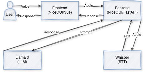
We will go into the integration of Llama 3 with a speech-to-text model, all within a user-friendly interface. This fusion enables (near) real-time communication with an LLM through speech. Our exploration involves selecting Llama 3 8B as the LLM, using the Whisper speech-to-text model, and the capabilities of NiceGUI — a framework that uses FastAPI on the backend and Vue3 on the frontend, interconnected with socket.io.
After reading this post, you will be able to augment an LLM with a new audio modality. This will allow you to build a full end-to-end workflow and UI that enables you to use your voice to command and prompt an LLM instead of typing. This feature can prove especially beneficial for mobile applications, where typing on a keyboard may not be as user-friendly as on desktops. Additionally, integrating this functionality can enhance the accessibility of your LLM app, making it more inclusive for individuals with disabilities.
Here are the tools and technologies that this project will help you get familiar with:
Llama 3 LLM
Whisper STT
NiceGUI
(Some) Basic Javascript and Vue3
The Replicate API
List of Components
In this project, we integrate various components to enable voice interaction with LLMs (Large Language Models). Firstly, LLMs serve as the core of our system, processing inputs and generating outputs based on extensive language knowledge. Next, Whisper, our chosen speech-to-text model, converts spoken input into text, enabling smooth communication with the LLMs. Our frontend, based on Vue3, incorporates custom components within the NiceGUI framework, providing an intuitive user interface for interaction. On the backend, custom code combined with FastAPI forms the base of the app’s functionality. Finally, Replicate.com provides the hosting infrastructure for the ML models, ensuring reliable access and scalability. Together, these components converge to create a basic app for (near) real-time voice interaction with LLMs.
In order to create such component, we just need to define a .vue file that defines what we want:
<template>
  <div>
    <button class="record-button" @mousedown="startRecording" @mouseup="stopRecording">Hold to speak</button>
  </div>
</template>
Here, basically, we create a button element where when clicked will call a method startRecording and as soon as the mouse is up will call stopRecording.
This code defines three methods: requestMicrophonePermission, startRecording, and stopRecording. The requestMicrophonePermission method asynchronously attempts to access the user’s microphone using navigator.mediaDevices.getUserMedia, handling any errors that may occur. The startRecording method, also asynchronous, initializes recording by setting up a media recorder with the obtained microphone stream, while the stopRecording method stops the recording process and saves the recorded audio.
Once the recording is done, this code will also emit an event named ‘audio_ready’ along with a base64 encoded audio data. Inside the method, a new FileReader object is created. Upon loading the file, the onload event is triggered, extracting the base64 data from the loaded file result. Finally, this base64 data is emitted as part of the ‘audio_ready’ event using $emit() function with the key ‘audioBlobBase64’ containing the base64 data.
emitBlob() {
      const reader = new FileReader();
      reader.onload = () => {
        const base64Data = reader.result.split(',')[1]; // Extracting base64 data from the result
        this.$emit('audio_ready', { audioBlobBase64: base64Data });
      };
    }
This event will be received by the backend along with the base64 data.
The backend
The backend will be basically the glue that ties the user’s input with the ML models hosted in Replicate.
We will be employing two primary models for our project:
openai/whisper: This Transformer sequence-to-sequence model is dedicated to speech-to-text tasks, proficient in converting audio into text. Trained across various speech processing tasks, such as multilingual speech recognition, speech translation, spoken language identification, and voice activity detection.
meta/meta-llama-3-8b-instruct: The Llama 3 family, including this 8 billion-parameter variant, is an LLM family created by Meta. These pretrained and instruction-tuned generative text models are specifically optimized for dialogue use cases.
For the first one, we define a simple function that takes as input the base64 audio and calls the replicate api:
def transcribe_audio(base64_audio):
    audio_bytes = base64.b64decode(base64_audio)
    prediction = replicate.run(
        f"{MODEL_STT}:{VERSION}", input={"audio": io.BytesIO(audio_bytes), **ARGS}
    )
    text = "n".join(segment["text"] for segment in prediction.get("segments", []))
    return text
Which can be used easily as:
with open("audio.ogx", "rb") as f: content = f.read()
Once the audio data is ready, we first transcribe the audio, then once this is done, we call the LLM and display its response. The variables self.prompt and self.response_html are bound to other NiceGUI components that get updated automatically. If you want to know more about how that works, you can look into a previous tutorial I wrote:
What takes the most time here is the audio transcription. The endpoint is always warm on replicate when I check it, but this version is the large-v3 which is not the fastest one. Audio files are also a lot heavier to move around than plain text, so this contributes to the small latency.
Notes:
You will need to set REPLICATE_API_TOKEN before running this code. You can get this by signing up in replicate.com. I was able to do these experiments using their free tier.
Sometimes the transcription is delayed a little bit and is returned after a short “Queuing” period.
In summary, the integration of open-source models like Whisper and Llama 3 has significantly simplified voice interaction with LLMs, making it highly accessible and user-friendly. This combination is particularly convenient for users who prefer not to type, offering a smooth experience. However, this is only the first part of the project; there will be more improvements to come. The next steps include enabling two-way voice communication, providing the option to utilize local models for enhanced privacy, enhancing the overall design for a more polished interface, implementing multi-turn conversations for more natural interactions, developing a desktop application for wider accessibility, and optimizing latency for real-time speech-to-text processing. With these enhancements, the aim is to improve the experience of voice interaction with LLMs, making it easier to use for those, like me, that don’t like typing that much. Let me know which improvements do you think I should work on first.
Presentation of the latest release of deepdespeckling
Optical and radar image of an agricultural area near Nîmes, France
Synthetic aperture radar (SAR) images are widely use in a large variety of sectors (aerospace, military, meteorology, etc.). The problem is this kind of images suffer from noise in their raw format. While these images are also usually heavy files, the task of denoising it efficiently appears to be both challenging from a scientific perspective and very useful in the real world.
In this Towards Data Science article, we presented deepdespeckling, an open-source python package enabling to despeckle synthetic aperture radar (SAR) images using a novel deep learning based method.
We are happy to announce that we have released a new version ofdeepdespeckling, enabling to use both MERLIN and SAR2SAR methods for despeckling radar satellite images.
A quick reminder on satellite images
There are two big categories of satellite images :
Optical images : the ones we are used to see when we watch a weather forecast for example. These images are taken by optical sensors. While these images generally provide a high level of detail, they encounter at least two significant challenges in capturing Earth’s intricacies: the limitations posed by nighttime conditions and adverse weather.
Radar images : while optical systems rely on the sunlight (the sensor is passive), radars send an electromagnetic wave and measure the component backscattered by the objects on the ground (the sensor is active). radar sensors can acquire data at any time of the day and with any meteorological conditions, as the wavelength of the transmitted wave allows it to penetrate clouds. They however encounter an intrinsic issue : speckle noise.
What is speckle noise ?
Speckle is a granular interference due to bouncing properties of emitted radio waves that degrades the quality of images and therefore their interpretability with a human eye.
Example of an image respectively without and with speckle noise
How to get rid of it
Several methods exist, but deep learning has brought significant improvements for this task. Emanuele Dalsasso, Loïc Denis and Florence Tupin developed two deep learning based methods for despeckling SAR images :
MERLIN (coMplex sElf-supeRvised despeckLINg) : a self-supervised strategy based on the separation of the real and imaginary parts of single-look complex SAR images that we presented in the previous Towards Data Science article
SAR2SAR : Multi-temporal time series are leveraged in order to train neural network to restore SAR images by only looking at noisy acquisitions. This method is part of the new features of the latest release of deepdespeckling. Hence, we will focus on this method in this article
SAR2SAR
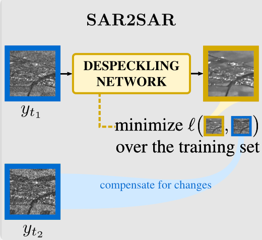
Just as MERLIN, SAR2SAR also draws inspiration from the noise2noise algorithm, which showed that it is possible to train a model to denoise without looking at noise-free examples. This feature is of particular importance in SAR despeckling, as speckle-free acquisition do not exist.
SAR2SAR builds on the assumption that two images acquired over the same area at different times are corrupted by two uncorrelated speckle realizations, matching with the hypothesis allowing the application of the noise2noise principle. This allows to develop a model to remove speckle from Ground Range Detected (GRD) SAR images, which are only available in amplitude (the phase is suppressed during the detection step) and thus MERLIN cannot be used on such data. Temporal acquisitions are leveraged to generate a dataset containing independent speckle realisations of the same scene (a change compensations strategy relying on a pre-trained model is used to ensure that the temporal acquisitions only differ for the speckle component).
Once the model is trained, during inference SAR2SAR requires a single GRD image and can be effectively deployed to suppress speckle from Sentinel-1 GRD SAR images.
SAR images acquisition
Different acquisition modes exist depending on the compromise between the illuminated scene (the swath) and and the image resolution. Each acquisition mode thus produces images having a different resolution, thus the appearance of objects is specific to each acquisition mode.
For this reason, a model specific for each modality must be developed. Given the simplicity of application of MERLIN, which requires single SAR images, datasets for each specific modality can be seamlessly collected. We have trained MERLIN on the following images:
TerraSAR-X images acquired in Stripmap mode
TerraSAR-X images acquired in HighResolution SpotLight mode
Sentinel-1 images acquired in TOPS mode
deepdespeckling package usage
Package installation
Before installing deepdespeckling, make sure to install gdal dependancies, it can be done using conda with the following command :
conda install -c conda-forge gdal
Then you can install the package this way :
pip install deepdespeckling
Despeckle one image with MERLIN
To despeckle SAR images using MERLIN, images need to be in .cos or .npy format.
Two parameters have to be set:
model_name : “spotlight” for SAR images retrieved with spotlight mode, “stripmap” for SAR images retrieved with stripmap mode or “Sentinel-TOPS” for images retrieved with TOPS mode
symetrise: during the preprocessing steps of the noisy image for MERLIN, the real and the imaginary parts are “symetrised” (to match the theoretical assumptions of MERLIN). To skip this step, the symetrise parameter can be set to False
from deepdespeckling.utils.load_cosar import cos2mat from deepdespeckling.utils.constants import PATCH_SIZE, STRIDE_SIZE from deepdespeckling.merlin.merlin_denoiser import MerlinDenoiser
# Path to one image (cos or npy file) image_path="path/to/cosar/image" # Model name, can be "spotlight", "stripmap" or "Sentinel-TOPS" model_name = "spotlight" symetrise = True
This snippet of code will store the despeckled image in a numpy array in the denoised_imagevariable.
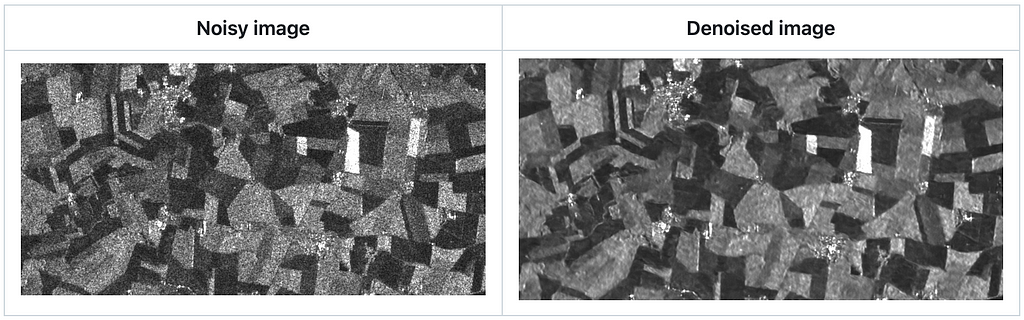
Example of a full size noisy SAR imageThe same image denoised using MERLIN
Despeckle one image with SAR2SAR
To despeckle SAR images using SAR2SAR, images need to be in .tiff or .npy format.
from deepdespeckling.utils.load_cosar import cos2mat
from deepdespeckling.utils.constants import PATCH_SIZE, STRIDE_SIZE
from deepdespeckling.sar2sar.sar2sar_denoiser import Sar2SarDenoiser

# Path to one image (tiff or npy file)
image_path="path/to/cosar/image"

# Works exactly the same as with MERLIN
image = cos2mat(image_path).astype(np.float32)

# Denoise the image with SAR2SAR
denoiser = Sar2SarDenoiser()
denoised_image = denoiser.denoise_image(image, patch_size=PATCH_SIZE, stride_size=STRIDE_SIZE)
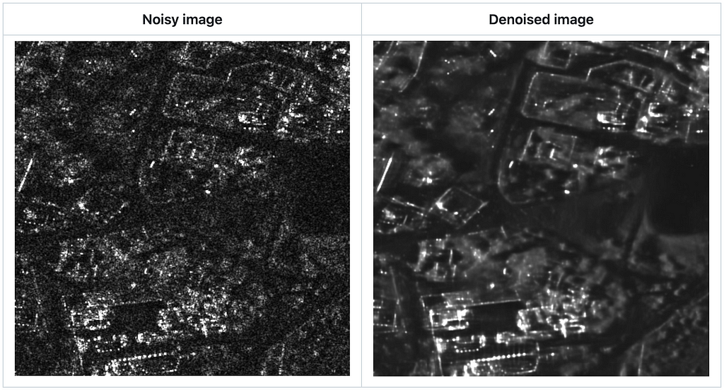
Example of result using SAR2SAR (displayed after a conversion to png)
Despeckle a set of images using MERLIN or SAR2SAR
For both MERLIN and SAR2SAR, you can choose between 3 different functions to despeckle a set of SAR images contained in a folder :
despeckle to despeckle full size images
despeckle_from_coordinates to despeckle a sub-part of the images defined by some coordinates
despeckle_from_crop to despeckle a sub-part of the images defined using a crop tool
Despeckle fullsize images
from deepdespeckling.despeckling import despeckle
# Path to a folder of several images # images have to be in .tiff or .npy formats if using sar2sar # images have to be in .cos or .npy formats is using merlin ("spotlight", "stripmap" or "Sentinel-TOPS") image_path="path/to/cosar/image" # Folder where results are stored destination_directory="path/where/to/save/results"
# Can be "sar2sar", "spotlight' or "stripmap" model_name = "spotlight" # symetrise parameter if using "spotlight", "stripmap" or "Sentinel-TOPS" (harmless if using "sar2sar") symetrise = True
The despeckle function will create several folders in the destination_directory :
processed_images: the npy files (numpy array conversion) of the raw images stored in the folder defined in image_path.
noisy:the preprocessed noisy images in both .npy and .png formats
denoised: the denoised images in both .npy and .png formats
Despeckle parts of images using custom coordinates
from deepdespeckling.despeckling import despeckle_from_coordinates
# Path to a folder of several images # images have to be in .tiff or .npy formats if using sar2sar # images have to be in .cos or .npy formats is using merlin ("spotlight", "stripmap" or "Sentinel-TOPS") image_path="path/to/cosar/image" # Folder where results are stored destination_directory="path/where/to/save/results" # Example of coordinates of the subparts of the images to be despeckled coordinates_dictionnary = {'x_start':2600,'y_start':1000,'x_end':3000,'y_end':1200}
# Can be "sar2sar", "spotlight", "stripmap" or "Sentinel-TOPS" model_name = "spotlight" # symetrise parameter if using "spotlight", "stripmap" or "Sentinel-TOPS" (harmless if using "sar2sar") symetrise = True
Thedespeckle_from_coordinates function will create the same folders as thedespeckle function, with images croped with the specified coordinates.
Example of image denoised using custom coordinates (displayed after a conversion to png)
Despeckle parts of images using a crop tool
from deepdespeckling.merlin.inference.despeckling import despeckle_from_crop
# Path to a folder of several images # images have to be in .tiff or .npy formats if using sar2sar # images have to be in .cos or .npy formats is using merlin ("spotlight", "stripmap" or "Sentinel-TOPS") image_path="path/to/cosar/image" # Folder where results are stored destination_directory="path/where/to/save/results"
# If True it will crop a 256*256 image from the position of your click # If False you will draw free-handly the area of your interest fixed = True # Can be "sar2sar", "spotlight", "stripmap" or "Sentinel-TOPS" model_name = "spotlight" # symetrise parameter if using "spotlight""stripmap" or "Sentinel-TOPS" (harmless if using "sar2sar") symetrise = True
Thedespeckle_from_crop function will first launch the crop tool : just select an area and press “q” when you are satisfied with the crop
the cropping tool in actionResults of the denoising using the crop tool
Then, the despeckle_from_crop function will create :
The same folders as thedespeckle function, with images cropped using the crop tool
cropping_coordinates.txt file containing the coordinates of the selected crop
Going further
Now you know to use deepdespeckling, to understand further more how it works, you can check the github repository. We also provide a sphinx documentation available here.
Feel free to contact me for any questions and feedback !
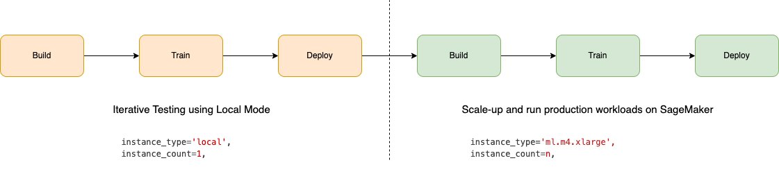
We are excited to announce two new capabilities in Amazon SageMaker Studio that will accelerate iterative development for machine learning (ML) practitioners: Local Mode and Docker support. ML model development often involves slow iteration cycles as developers switch between coding, training, and deployment. Each step requires waiting for remote compute resources to start up, which […]
A practical assessment of Differential Privacy & Federated Learning in the medical context.
(Bing AI generated image, original, full ownership)
Sensitive data cries out for more protection
The need for data privacy seems to be generally at ease nowadays in the era of large language models trained on everything from the public internet, regardless of actual intellectual property which their respective company leaders openly admit.
But there’s a much more sensitive parallel universe when it comes to patients’ data, our health records, which are undoubtedly much more sensitive and in need of protection.
Also the regulations are getting stronger all over the world, the trend is unanimously towards more stricter data protection regulations, including AI.
There are obvious ethical reasons which we don’t have to explain, but from the enterprise levels regulatory and legal reasons that require pharmaceutical companies, labs and hospitals to use state of the art technologies to protect data privacy of patients.
Federated paradigm is here to help
Federated analytics and learning are great options to be able to analyze data and train models on patients’ data without accessing any raw data.
In case of federated analytics it means, for instance, we can get correlation between blood glucose and patients BMI without accessing any raw data that could lead to patients re-identification.
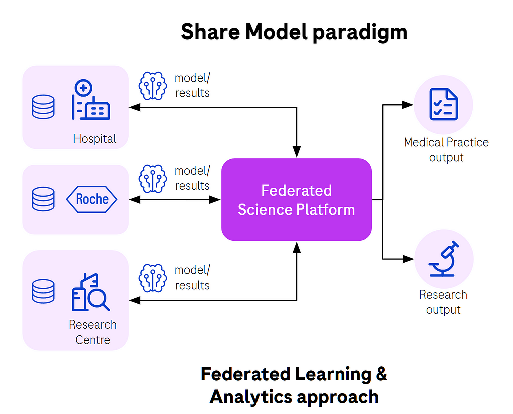
In the case of machine learning, let’s use the example of diagnostics, where models are trained on patients’ images to detect malignant changes in their tissues and detect early stages of cancer, for instance. This is literally a life saving application of machine learning. Models are trained locally at the hospital level using local images and labels assigned by professional radiologists, then there’s aggregation which combines all those local models into a single more generalized model. The process repeats for tens or hundreds of rounds to improve the performance of the model.
Fig. 1. Federated learning in action, sharing model updates, not data.
The reward for each individual hospital is that they will benefit from a better trained model able to detect disease in future patients with higher probability. It’s a win-win situation for everyone, especially patients.
Of course there’s a variety of federated network topologies and model aggregation strategies, but for the sake of this article we tried to focus on the typical example.
Federated learning is a key strategy to build that trust backed up by the technology, not only on contracts and faith in ethics of particular employees and partners of the organizations forming consortia.
First of all, the data remains at the source, never leaves the hospital, and is not being centralized in a single, potentially vulnerable location. Federated approach means there aren’t any external copies of the data that may be hard to remove after the research is completed.
The technology blocks access to raw data because of multiple techniques that follow defense in depth principle. Each of them is minimizing the risk of data exposure and patient re-identification by tens or thousands of times. Everything to make it economically unviable to discover nor reconstruct raw level data.
Data is minimized first to expose only the necessary properties to machine learning agents running locally, PII data is stripped, and we also use anonymization techniques.
Then local nodes protect local data against the so-called too curious data scientist threat by allowing only the code and operations accepted by local data owners to run against their data. For instance model training code deployed locally at the hospital as a package is allowed or not by the local data owners. Remote data scientists cannot just send any code to remote nodes as that would allow them for instance to return raw level data. This requires a new, decentralized way of thinking to embrace different mindset and technologies for permission management, an interesting topic for another time.
Are models private enough?
Assuming all those layers of protection are in place there’s still concern related to the safety of model weights themselves.
There’s growing concern in the AI community about machine learning models as the super compression of the data, not as black-boxy as previously considered, and revealing more information about the underlying data than previously thought.
And that means that with enough skills, time, effort and powerful hardware a motivated adversary can try to reconstruct the original data, or at least prove with high probability that a given patient was in the group that was used to train the model (Membership Inference Attack (MIA)) . Other types of attacks possible such as extraction, reconstruction and evasion.
To make things even worse, the progress of generative AI that we all admire and benefit from, delivers new, more effective techniques for image reconstruction (for example, lung scan of the patients). The same ideas that are used by all of us to generate images on demand can be used by adversaries to reconstruct original images from MRI/CT scan machines. Other modalities of data such as tabular data, text, sound and video can now be reconstructed using gen AI.
Differential Privacy to the rescue
Differential privacy (DP) algorithms promise that we exchange some of the model’s accuracy for much improved resilience against inference attacks. This is another privacy-utility trade-off that is worth considering.
It can be as easy as least effective Gaussian noise but nowadays we embrace the development of much more sophisticated algorithms such as Sparse Vector Technique (SVT), Opacus library as practical implementation of differentially private stochastic gradient descent (DP-SGD), plus venerable Laplacian noise based libraries (i.e. PyDP).
Fig. 2. On device differential privacy that we all use all the time.
And, by the way, we all benefit from this technique without even realizing that it even exists, and it is happening right now. Our telemetry data from mobile devices (Apple iOS, Google Android) and desktop OSes (Microsoft Windows) is using differential privacy and federated learning algorithms to train models without sending raw data from our devices. And it’s been around for years now.
Now, there’s growing adoption for other use cases including our favorite siloed federated learning case, with relatively few participants with large amounts of data in on-purpose established consortia of different organizations and companies.
Differential privacy is not specific to federated learning. However, there are different strategies of applying DP in federated learning scenarios as well as different selection of algorithms. Different algorithms which work better for federated learning setups, different for local data privacy (LDP) and centralized data processing.
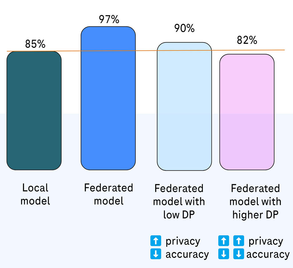
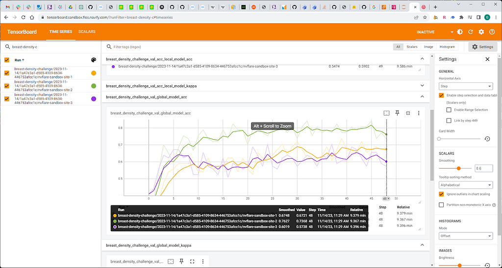
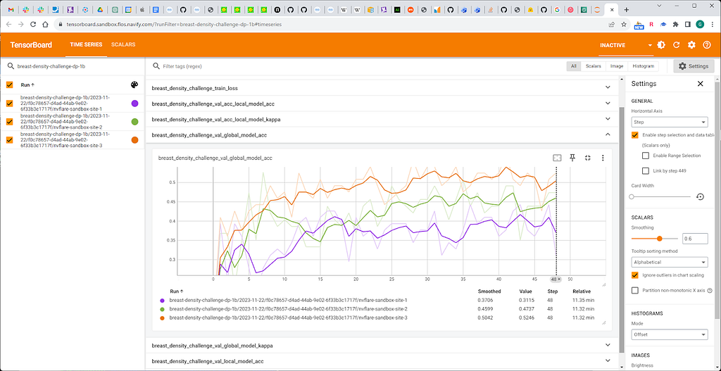
In the context of federated learning we anticipate a drop in model accuracy after applying differential privacy, but still (and to some extent hopefully) expect the model to perform better than local models without federated aggregation. So the federated model should still retain its advantage despite added noise and clipping (DP).
Fig. 3. What we can expect based on known papers and our experiences.
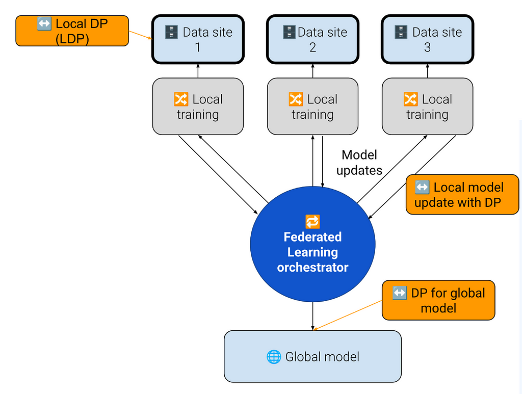
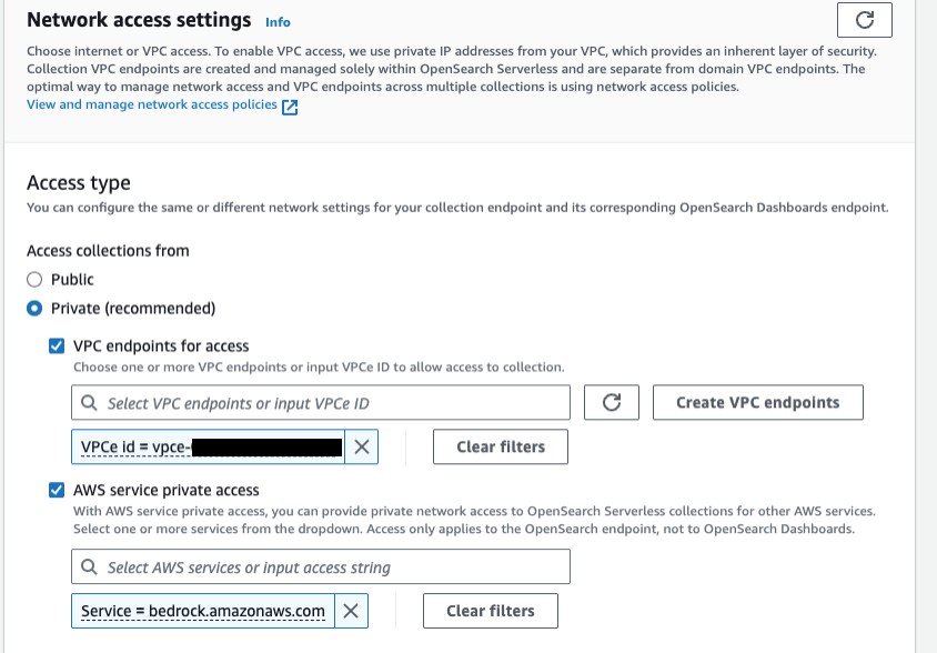
Differential privacy can be applied as early as at the source data (Local Differential Privacy (LDP)).
Fig. 4, different places where DP can be applied to improve data protection
There are also cases of federated learning within a network of partners who have all data access rights and are less concerned about data protection levels so there might be no DP at all.
On the other hand when the model is going to be shared with the outside world or sold commercially it might be a good idea to apply DP for the global model as well.
Practical experimentation results
At Roche’s Federated Open Science team, NVIDIA Flare is our tool of choice for federated learning as the most mature open source federated framework on the market. We also collaborate with the NVIDIA team on future development of NVIDIA Flare and are glad to help to improve an already great solution for federated learning.
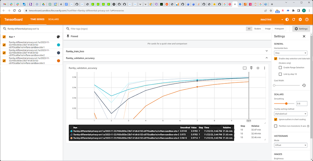
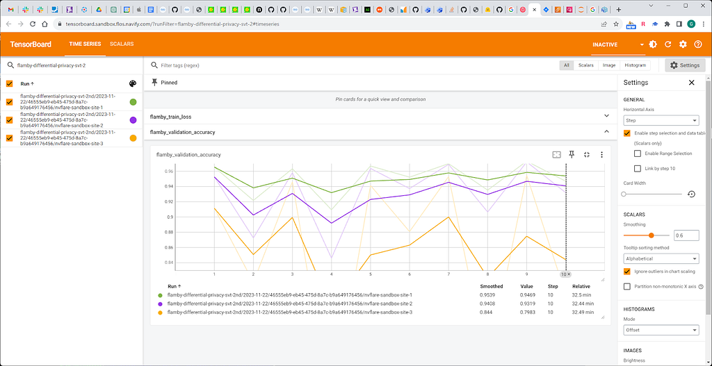
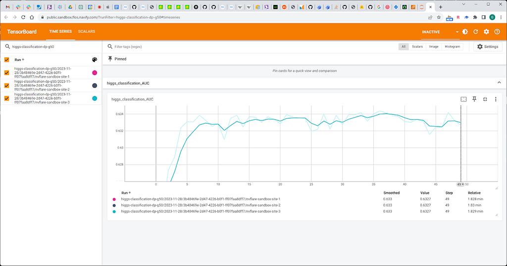
Fig. 10. Models performance with percentile value 95.
Fig. 11. Percentile value 50.
We observe minor, acceptable accuracy loss related to DP.
Lessons learned
Important lesson learned is that differential privacy outcomes are very sensitive to parameters of a given DP algorithm and it’s hard to tune it to avoid total collapse of model accuracy.
Also, we experienced some kind of anxiety, based on the impression of not really really knowing how much privacy protection we have gained for what price. We only saw the “cost” side (accuracy degradation).
We had to rely to a major extent on known literature, that says and demonstrated, that even small amounts of DP-noise are helping to secure data.
As engineers, we’d like to see some type of automatic measure that would prove how much privacy we gained for how much accuracy lost, and maybe even some kind of AutoDP tuning. Seems to be far, far away from the current state of technology and knowledge.
Then we applied privacy meters to see if there’s a visible difference between models without DP versus models with DP and we observed changes in the curve, but it’s really hard to quantify how much we gained.
Some algorithms didn’t work at all, some required many attempts to tune them properly to deliver viable results. There was no clear guidance on how to tune different parameters for particular dataset and ML models.
So our current opinion is that DP for FL is hard, but totally feasible. It requires a lot of iterations, and trial and error loops to achieve acceptable results while believing in privacy improvements of orders of magnitude based on the trust in algorithms.
The future
Federated learning is a great option to improve patients’ outcomes and treatment efficacy because of the improved ML models while preserving patients’ data.
But data protection never comes without any price and differential privacy for federated learning is a perfect example of that trade-off.
It’s great to see improvements in algorithms of differential privacy for federated learning scenarios to minimize the impact on accuracy while maximizing resilience of models against inference attacks.
As with all trade-offs the decisions have to be made balancing usefulness of models for practical applications against the risks of data leakage and reconstruction.
And that’s where our expectation for privacy meters are growing to know more precisely what we are selling and we are “buying”, what the exchange ratio is.
The landscape is dynamic, with better tools available for both those who want to better protect their data and those who are motivated to violate those rules and expose sensitive data.
We also invite other federated minds to build upon and contribute to the collective effort of advancing patient data privacy for Federated Learning.
The author would like to thank Jacek Chmiel for significant impact on the blog post itself, as well as the people who helped develop these ideas and bring them to practice: Jacek Chmiel, Lukasz Antczak and Grzegory Gajda.
All images in this article were created by the authors.
We introduced Amazon Bedrock to the world a little over a year ago, delivering an entirely new way to build generative artificial intelligence (AI) applications. With the broadest selection of first- and third-party foundation models (FMs) as well as user-friendly capabilities, Amazon Bedrock is the fastest and easiest way to build and scale secure generative […]
This post explores the new enterprise-grade features for Knowledge Bases on Amazon Bedrock and how they align with the AWS Well-Architected Framework. With Knowledge Bases for Amazon Bedrock, you can quickly build applications using Retrieval Augmented Generation (RAG) for use cases like question answering, contextual chatbots, and personalized search.
From data to decisions: maximizing rewards with policy improvement methods for optimal strategies
Introduction
Reinforcement learning is a domain in machine learning that introduces the concept of an agent who must learn optimal strategies in complex environments. The agent learns from its actions that result in rewards given the environment’s state. Reinforcement learning is a difficult topic and differs significantly from other areas of machine learning. That is why it should only be used when a given problem cannot be solved otherwise.
The incredible flexibility of reinforcement learning is that the same algorithms can be used to make the agent adapt to completely different, unknown, and complex conditions.
Note. To fully understand the ideas included in this article, it is highly recommended to be familiar with the main concepts of reinforcement learning introduced in the first part of this article series.
In Part 1, we have introduced the main concepts of reinforcement learning: the framework, policies and value functions. The Bellman equation that recursively establishes the relationship of value functions is the backbone of modern algorithms. We will understand its power in this article by learning how it can be used to find optimal policies.
This article is based on Chapter 4 of the book “Reinforcement Learning” written by Richard S. Sutton and Andrew G. Barto. I highly appreciate the efforts of the authors who contributed to the publication of this book.
Solving Bellman equation
Let us imagine that we perfectly know the environment’s dynamics that contains |S| states. Action transition probablities are given by a policy π. Given that, we can solve the Bellman equation for the V-function for this environment that will, in fact, represent a system of linear equations with |S| variables (in case of the Q-function there will be |S| x |A| equations).
The solution to that system of equations corresponds to v-values for every state (or q-values for every pair (state, pair)).
Example
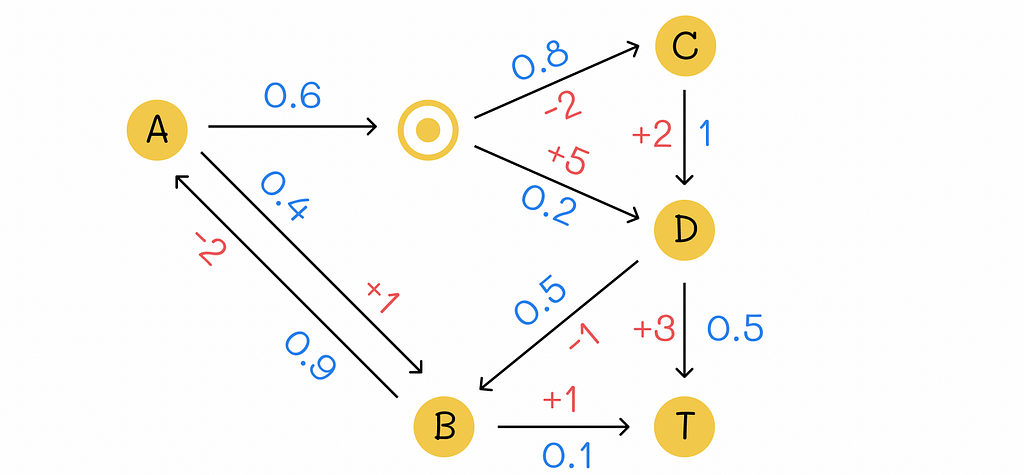
Let us have a look at a simple example of an environment with 5 states where T is a terminal state. Numbers in blue represent transition probabilities while number in red represent rewards received by the agent. We will also assume that the same action chosen by the agent in the state A (represented by the horizontal arrow with probability p = 0.6) leads to either C or D with different probabilities (p = 0.8 and p = 0.2).
Transition diagram for the example. Numbers in blue denote transition probabilities between states and numbers in red define respective rewards.
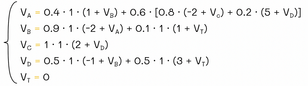
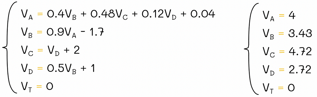
Since the environment contains |S|= 5 states, to find all v-values, we will have to solve a system of equations consisting of 5 Bellman equations:
System of Bellman equations for the V-function.
Since T is a terminal state, its v-value is always 0, so technically we only have to solve 4 equations.
Solution of the system of equations.
Solving the analogous system for the Q-function would be harder because we would need to solve an equation for every pair (state, action).
Policy evaluation
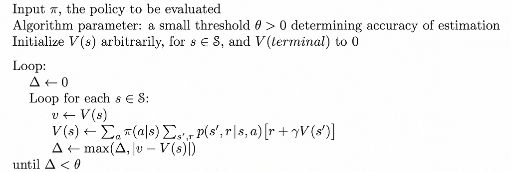
Solving a linear system of equations in a straightforward manner, as it was shown in the example above, is a possible way to get real v-values. However, given the cubic algorithm complexity O(n³), where n = |S|, it is not optimal, especially when the number of states |S| is large. Instead, we can apply an iterative policy evaluation algorithm:
Randomly initialise v-values for all environment states (except for terminal states whose v-values must be equal to 0).
Iteratively update all non-terminal states by using the Bellman equation.
Repeat step 2 until the difference between previous and current v-values is too small (≤ θ).
If the number of states |S| if finite, then it is possible to prove mathematically that iterative estimations obtained by the policy evaluation algorithm under a given policy πultimately converge to real v-values!
A single update of the v-value of a state s ∈ S is called an expected update. The logic behind this name is that the update procedure considers rewards of all possible successive states of s, not just a single one.
A whole iteration of updates for all states is called a sweep.
Note. The analogous iterative algorithm can be applied to the calculation of Q-functions as well.
To realize how amazing this algorithm is, let us highlight it once again:
Policy evaluation allows iteratively finding the V-function under a given policy π.
Update variations
The update equation in the policy evaluation algorithm can be implemented in two ways:
By using two arrays: new values are computed sequentially from unchanged old values stored in two separate arrays.
By using one array: computed values are overwritten immediately. As a result, later updates during the same iteration use the overwritten new values.
In practice, overwriting v-values is a preferable way to perform updates because the new information is used as soon as it becomes available for other updates, in comparison to the two array method. As a consequence, v-values tend to converge faster.
The algorithm does not impose rules on the order of variables that should be updated during every iteration, however the order can have a large influence on the convergence rate.
Example
Description
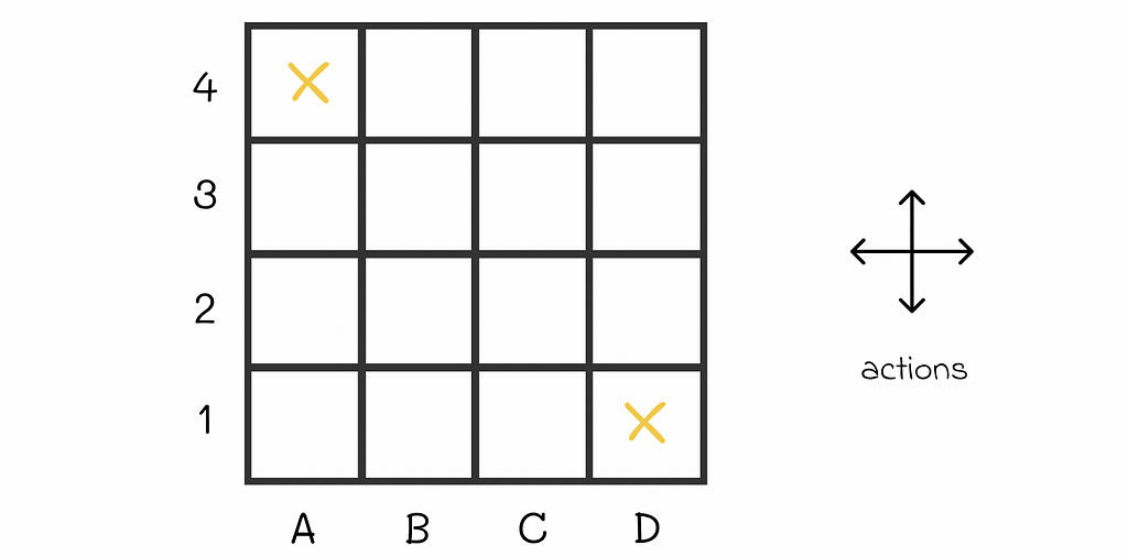
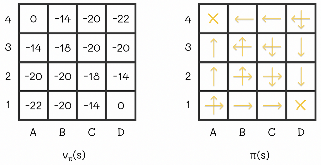
To further understand how the policy evaluation algorithm works in practice, let us have a look at the example 4.1 from the Sutton’s and Barto’s book. We are given an environment in the form of the 4 x 4 grid where at every step the agent equiprobably (p = 0.25) makes a single step in one of the four directions (up, right, down, left).
If an agent is located at the edge of the maze and chooses to go into the direction of a wall around the maze, then its position stays the same. For example, if the agent is located at D3 and chooses to go to the right, then it will stay at D3 at the next state.
Every move to any cell results in R = -1 reward except for two terminal states located at A4 and D1 whose rewards are R = 0. The ultimate goal is to calculate V-function for the given equiprobable policy.
Algorithm
Let us initialize all V-values to 0. Then we will run several iterations of the policy evaluation algorithm:
At some point, there will be no changes between v-values on consecutive iterations. That means that the algorithm has converged to the real V-values. For the maze, the V-function under the equiprobable policy is shown at the right of the last diagram row.
Interpretation
Let us say an agent acting according to the random policy starts from the cell C2 whose expected reward is -18. By the V-function definition, -18 is the total cumulative reward the agent receives by the end of the episode. Since every move in the maze adds -1 to the reward, we can interpret the v-value of 18 as the expected number of steps the agent will have to make until it gets to the terminal state.
Policy improvement
At first sight, it might sound surprising but V- and Q- functions can be used to find optimal policies. To understand this, let us refer to the maze example where we have calculated the V-function for a starting random policy.
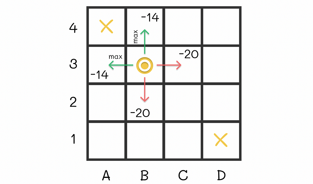
For instance, let us take the cell B3. Given our random policy, the agent can go in 4 directions with equal probabilities from that state. The possible expected rewards it can receive are -14, -20, -20 and -14. Let us suppose that we had an option to modify the policy for that state. To maximize the expected reward, would not it be logical to always go next to either A3 or B4 from B3, i.e. in the cell with the maximum expected reward in the neighbourhood (-14 in our case)?
Optimal actions from the cell B3 lead to either A3 or B4 where the expected reward reaches its maximum.
This idea makes sense because being located at A3 or B4 gives the agent a possibility to finish the maze in just one step. As a result, we can include that transition rule for B3 to derive a new policy. Nevertheless, is it always optimal to make such transitions to maximize the expected reward?
Indeed, transitioning greedily to the state with an action whose combination of expected reward is maximal among other possible next states, leads to a better policy.
To continue our example, let us perform the same procedure for all maze states:
As a consequence, we have derived a new policy that is better than the old one. By the way, our findings can be generalized for other problems as well by the policy improvement theorem which plays a crucial role in reinforcement learning.
To understand the theorem’s formulation, let us assume that we have access to the V- and Q-functions of a given environment evaluated under a policy π. For that environment, we will create another policy π’. This policy will be absolutely the same as π with the only difference that for every state it will choose actions that result in either the same or greater rewards. Then the theorem guarantees that the V-function under policy π’ will be better than the one for the policy π.
With the policy improvement theorem, we can always derive better policies by greedily choosing actions of the current policy that lead to maximum rewards for every state.
Policy iteration
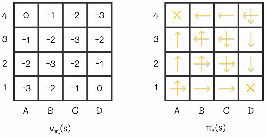
Given any starting policy π, we can compute its V-function. This V-function can be used to improve the policy to π’. With this policy π’, we can calculate its V’-function. This procedure can be repeated multiple times to iteratively produce better policies and value functions.
In the limit, for a finite number of states, this algorithm, called policy iteration, converges to the optimal policy and the optimal value function.
In these settings, with the obtained optimal V-function, we can easily estimate the number of steps required to get to the terminal state, according to the optimal strategy.
What is so interesting about this example is the fact that we would only need two policy iterations to obtain these values from scratch (we can notice that the optimal policy from the image is exactly the same as it was before when we had greedily updated it to the respective V-function). In some situations, the policy iteration algorithm requires only few iterations to converge.
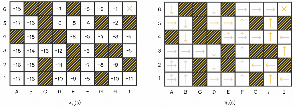
An example of the optimal V-function and policy for a more complex maze environment.
Value iteration
Though the original policy iteration algorithm can be used to find optimal policies, it can be slow, mainly because of multiple sweeps performed during policy evaluation steps. Moreover, the full convergence process to the exact V-function might require a lot sweeps.
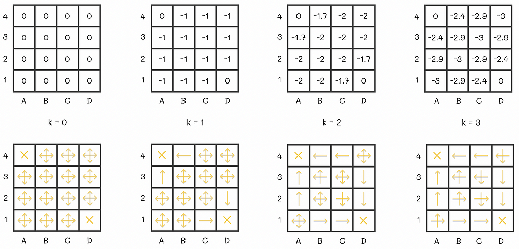
In addition, sometimes it is not necessary to get exact v-values to yield a better policy. The previous example demonstrates it perfectly: instead of performing multiple sweeps, we could have done only k = 3 sweeps and then built a policy based on the obtained approximation of the V-function. This policy would have been exactly the same as the one we have computed after V-function convergence.
V-function and policy evaluations on the first three iterations. We can see that starting from the third iteration, the policy does not change. This example demonstrates that in some cases it is not necessary to run all iterations of policy iteration. Image adapted by the author. Source: Reinforcement Learning. An Introduction. Second Edition | Richard S. Sutton and Andrew G. Barto
In general, is it possible to stop the policy evaluation algorithm at some point? It turns out that yes! Furthermore, only a single sweep can be performed during every policy evaluation step and the result will still converge to the optimal policy. The described algorithm is called value iteration.
We are not going to study the proof of this algorithm. Nevertheless, we can notice that policy evaluation and policy improvement are two very similar processes to each other: both of them use the Bellman equation except for the fact that policy improvement takes the max operation to yield a better action.
By iteratively performing a single sweep of policy evaluation and a single sweep of policy improvement, we can converge faster to the optimum. In reality, we can stop the algorithm once the difference between successive V-functions becomes insignificant.
Asynchronous value iteration
In some situations, performing just a single sweep during every step of value iteration can be problematic, especially when the number of states |S| is large. To overcome this, asynchronous versions of the algorithm can be used: instead of systematically performing updates of all states during the whole sweep, only a subset ofstate values is updated in-place in whatever order. Moreover, some states can be updated multiple times before other states are updated.
However, at some point, all of the states will have to be updated, to make it possible for the algorithm to converge. According to the theory, all of the states must be updated in total an infinite number of times to achieve convergence but in practice this aspect is usually omitted since we are not always interested in getting 100% optimal policy.
There exist different implementations of asynchronous value iteration. In real problems, they make it possible to efficiently trade off between the algorithm’s speed and accuracy.
One of the the simplest asynchronous versions is to update only a single state during the policy evaluation.
Generalized policy iteration
We have looked at the policy iteration algorithm. Its idea can be used to refer to a broader term in reinforcement learning called generalized policy iteration (GPI).
The GPI consists of finding the optimal policy through independent alternation between policy evaluation and policy improvement processes.
Almost all of the reinforcement learning algorithms can be referred to as GPI.
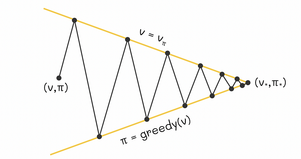
Sutton and Barto provide a simplified geometric figure that intuitively explains how GPI works. Let us imagine a 2D plane where every point represents a combination of a value function and a policy. Then we will draw two lines:
The first line will contain points corresponding to different V-functions of an environment.
The second line will represent a set of greedy policies in relation to respective V-functions.
Every time when we calculate a greedy policy for the current V-function, we move closer to the policy line while moving away from the V-function line. That is logical because for the new computed policy, the previous V-function no longer applies. On the other hand, every time we perform policy evaluation, we move towards the projection of a point on the V-function line and thus we move further from the policy line: for the new estimated V-function, the current policy is no longer optimal. The whole process is repeated again.
As these two processes alternate between each other, both current V-function and policy gradually improve and at some moment in time they must reach a point of optimality that will represent an intersection between the V-function and policy lines.
Conclusion
In this article, we have gone through the main ideas behind policy evaluation and policy improvement. The beauty of these two algorithms is their ability to interact with each other to reach the optimal state. This approach only works in perfect environments where the agent’s probability transitions are given for all states and actions. Despite this constraint, many other reinforcement learning algorithms use the GPI method as a fundamental building block for finding optimal policies.
For environments with numerous states, several heuristics can be applied to accelerate the convergence speed one of which includes asynchronous updates during the policy evaluation step. Since the majority of reinforcement algorithms require a lot of computational resources, this technique becomes very useful and allows efficiently trading accuracy for gains in speed.
A step-by-step guide to linking your AI agent with a SQL database — Part 2 of the series
Imagine streamlining your entire business management through a single, user-friendly interface on your phone. While juggling multiple apps is common practice, the future lies in consolidating all your interactions into one chat-based platform, powered by the capabilities of Large Language Models (LLMs).
For small businesses, this approach offers significant advantages. By centralizing data management tasks within a unified chat interface, owners can save time, reduce complexity, and minimize reliance on disparate software tools. The result is a more efficient allocation of resources, allowing a greater focus on core business growth activities.
However, the potential extends beyond just small businesses. The concepts and techniques detailed in this tutorial are adaptable to personal use cases as well. From managing to-do lists and tracking expenses to organizing collections, a chat-based interface provides an intuitive and efficient way to interact with your data.
This article is the second installment in a series that guides you through the process of developing such a software project, from initial concept to practical implementation. Building upon the components introduced in the previous article, we will establish the foundational elements of our application, including:
Setting up the database schema
Defining core application functionality
Structuring the project repository
Creating Tools capable of interacting with multiple SQL database tables using natural language commands
By the end of this tutorial, you will have a clear understanding of how to architect a chat-based interface that leverages LLMs to simplify data management tasks. Whether you’re a small business owner looking to streamline operations or an individual seeking to optimize personal organization, the principles covered here will provide a solid starting point for your own projects.
Let’s begin by briefly recapping the key takeaways from the previous article to set the context for our current objectives.
Recap
In the first part of this series, we built a prototype agent workflow capable of interacting with tool objects. Our goal was to reduce hallucination in tool arguments generated by the underlying language model, in our case gpt-3.5-turbo.
To achieve this, we implemented two key changes:
Removed required parameters in the tool schema
Added a parameter validation step before executing the desired function
By setting all tool parameters to optional and manually checking for missing parameters, we eliminated the urge for the Agent/LLM to hallucinate missing values.
The key objects introduced in the previous article were:
OpenAiAgent: The main agent workflow class
Tool: A class representing a tool the agent can use
ToolResult and StepResult: Classes for encapsulating tool execution results
These components formed the foundation of our agent system, allowing it to process user requests, select appropriate tools, and generate responses.
With this recap in mind, let’s dive into the next phase of our project — integrating database functionality to store and manage business data.
Why Chat Interface for Small Business Data Management
Small businesses often face unique challenges when it comes to data maintenance. Like larger corporations, they need to regularly update and maintain various types of data, such as accounting records, time tracking, invoices, and more. However, the complexity and costs associated with modern ERP (Enterprise Resource Planning) systems can be prohibitive for small businesses. As a result, many resort to using a series of Excel spreadsheets to capture and maintain essential data.
The problem with this approach is that small business owners, who are rarely dedicated solely to administrative tasks, cannot afford to invest significant time and effort into complex administration and control processes. The key is to define lean processes and update data as it arises, minimizing the overhead of data management.
By leveraging the power of Large Language Models and creating a chat interface, we aim to simplify and streamline data management for small businesses. The chatbot will act as a unified interface, allowing users to input data, retrieve information, and perform various tasks using natural language commands. This eliminates the need for navigating multiple spreadsheets or developing complex web applications with multiple forms and dashboards.
Throughout this series, we will gradually enhance the chatbot’s capabilities, adding features such as role-based access control, advanced querying and evaluation, multimodal support, and integration with popular communication platforms like WhatsApp. By the end of the series, you will have a powerful and flexible tool that can adapt to your specific needs, whether you’re running a small business or simply looking to organize your personal life more efficiently.
Let’s get started!
1. Project Structure
To ensure a well-organized and maintainable project, we’ve structured our repository to encapsulate different functionalities and components systematically. Here’s an overview of the repository structure:
project-root/
│
├── database/
│ ├── db.py # Database connection and setup
│ ├── models.py # Database models/schemas
| └── utils.py # Database utilities
│
├── tools/
│ ├── base.py # Base class for tools
│ ├── add.py # Tool for adding data to the database
│ ├── query.py # Tool for querying data from the database
| └── utils.py # Tool utilities
│
├── agents/
│ ├── base.py # Main AI agent logic
│ ├── routing.py # Specialized agent for routing tasks
│ ├── task.py # Tool wrapper for OpenAI subagents
| └── utils.py # agent utilities
│
└── utils.py # Utility functions and classes
This structure allows for a clear separation of concerns, making it easier to develop, maintain, and scale our application.
2. Set up Database
Choosing the right database and ORM (Object-Relational Mapping) library is crucial for our application. For this project, we’ve selected the following frameworks:
SQLAlchemy: A powerful SQL toolkit and Object-Relational Mapping (ORM) library for Python. It provides a set of tools for interacting with databases using Python objects and classes.
SQLModel: A library that builds on top of SQLAlchemy and Pydantic, offering a simple and intuitive way to define database models and perform database operations.
By leveraging SQLModel, we can seamlessly integrate with Pydantic and SQLAlchemy, enabling efficient data validation and database operations while eliminating the risk of SQL injection attacks. Moreover, SQLModel allows us to easily build upon our previously designed Tool class, which uses Pydantic models for creating a tool schema.
To ensure the security and robustness of our application, we implement the following measures:
Role-based access control: Executable operations are bound to user roles, ensuring that users can only perform actions they are authorized to do. This adds an extra layer of security and prevents unauthorized access to sensitive data.
Prevention of SQL injection attacks: By utilizing ChatGPT’s natural language understanding capabilities, we can validate and sanitize user inputs, mitigating the risk of SQL injection vulnerabilities. SQLModel’s integration with Pydantic helps us enforce strict data validation rules.
With our tech stack decided, let’s dive into setting up the database and defining our models.
2.1 Database Models
To begin building our prototype application, we’ll define the essential database tables and their corresponding SQLModel definitions. For this tutorial, we’ll focus on three core tables:
Expense
Revenue
Customer
These tables will serve as the foundation for our application, allowing us to demonstrate the key functionalities and interactions.
Create a new file named models.py in the database directory and define the tables using SQLModel:
# databasemodels.py from typing import Optional
from pydantic import BeforeValidator, model_validator from sqlmodel import SQLModel, Field from datetime import time, datetime from typing_extensions import Annotated
def validate_date(v): if isinstance(v, datetime): return v
for f in ["%Y-%m-%d", "%Y-%m-%d %H:%M:%S"]: try: return datetime.strptime(v, f) except ValueError: pass
raise ValueError("Invalid date format")
def numeric_validator(v): if isinstance(v, int): return float(v) elif isinstance(v, float): return v raise ValueError("Value must be a number")
class Expense(SQLModel, table=True): id: Optional[int] = Field(primary_key=True, default=None) description: str net_amount: Numeric = Field(description="The net amount of the expense") gross_amount: Numeric tax_rate: Numeric date: DateFormat
In addition to the standard SQLModel fields, we’ve defined three custom type annotations: DateFormat, TimeFormat, and Numeric. These annotations leverage Pydantic’s BeforeValidator to ensure that the input data is correctly formatted before being stored in the database. The validate_date function handles the conversion of string input to the appropriate datetime. This approach allows us to accept a variety of date formats from the Large Language Model, reducing the need for strict format enforcement in the prompts.
2.2 Database Engine
With our models defined, we need a script to set up the database engine and create the corresponding tables. Let’s create a db.py file in the database directory to handle this:
# database/db.py from database.models import * from sqlmodel import SQLModel, create_engine import os
# local stored database DATABASE_URL = "sqlite:///app.db"
In this script, we import our models and the necessary SQLModel components. We define the DATABASE_URL to point to a local SQLite database file named app.db. We create an engine using create_engine from SQLModel, passing in the DATABASE_URL. The echo=True parameter enables verbose output for debugging purposes.
The create_db_and_tables function uses SQLModel.metadata.create_all to generate the corresponding tables in the database based on our defined models. Finally, we call this function to ensure the database and tables are created when the script is run.
With our database setup complete, we can now focus on updating our Tool class to work seamlessly with SQLModel and enhance our tool schema conversion process.
3. Tool Class
In this section, we’ll discuss the updates made to the Tool class to handle SQLModel instances and improve the validation process. For a more detailed explanation of the Tool class, visit my previous article.
First, we’ve added Type[SQLModel] as a possible type for the model field using the Union type hint. This allows the Tool class to accept both Pydantic’s BaseModel and SQLModel’s SQLModel as valid model types.
Next, we’ve introduced a new attribute called exclude_keys of type list[str] with a default value of [“id”]. The purpose of this attribute is to specify which keys should be excluded from the validation process and the OpenAI tool schema generation. In this case the default excluded key is id since for data entry creation with SqlModel the id is automatically generated during ingestion.
On top of that we introduced parse_model boolean attribute to our Tool class. Where we can basically decided if the tool function is called with our pydantic/SQLModel or with keyword arguments.
In the validate_input() method, we’ve added a check to ensure that the keys specified in exclude_keys are not considered as missing keys during the validation process. This is particularly useful for fields like id, which are automatically generated by SQLModel and should not be required in the input.
Similarly, in the openai_tool_schema property, we’ve added a loop to remove the excluded keys from the generated schema. This ensures that the excluded keys are not included in the schema sent to the OpenAI API. For recap we use the openai_tool_schema property to remove required arguments from our tool schema. This is done to elimenate hallucination by our language model.
Moreover, we changed the import from from pydantic.v1 import BaseModel to from pydantic import BaseModel. Since SQLModel is based on Pydantic v2, we want to be consistent and use Pydantic v2 at this point.
Here’s the updated code for the Tool class:
# tools/base.py from typing import Type, Callable, Union
from tools.convert import convert_to_openai_tool from pydantic import BaseModel, ConfigDict from sqlmodel import SQLModel
class ToolResult(BaseModel): content: str success: bool
def run(self, **kwargs) -> ToolResult: if self.validate_missing and model is not None: missing_values = self.validate_input(**kwargs) if missing_values: content = f"Missing values: {', '.join(missing_values)}" return ToolResult(content=content, success=False)
if self.parse_model: if hasattr(self.model, "model_validate"): input_ = self.model.model_validate(kwargs) else: input_ = self.model(**kwargs) result = self.function(input_)
else: result = self.function(**kwargs) return ToolResult(content=str(result), success=True)
def validate_input(self, **kwargs): if not self.validate_missing or not self.model: return [] model_keys = set(self.model.__annotations__.keys()) - set(self.exclude_keys) input_keys = set(kwargs.keys()) missing_values = model_keys - input_keys return list(missing_values)
@property def openai_tool_schema(self): schema = convert_to_openai_tool(self.model) # set function name schema["function"]["name"] = self.name
# remove required field if schema["function"]["parameters"].get("required"): del schema["function"]["parameters"]["required"] # remove exclude keys if self.exclude_keys: for key in self.exclude_keys: if key in schema["function"]["parameters"]["properties"]: del schema["function"]["parameters"]["properties"][key] return schema
These updates to the Tool class provide more flexibility and control over the validation process and schema generation when working with SQLModel instances.
3.1 Custom Tool Schema Conversion
In our Tool class, we create a schema from a Pydantic model using the convert_to_openai_tool function from Langchain. However, this function is based on Pydantic v1, while SQLModel uses Pydantic v2. To make the conversion function compatible, we need to adapt it. Let’s create a new script called convert.py:
# tools/convert.py
from langchain_core.utils.function_calling import _rm_titles
from typing import Type, Optional
from langchain_core.utils.json_schema import dereference_refs
from pydantic import BaseModel

def convert_to_openai_tool(
        model: Type[BaseModel],
        *,
        name: Optional[str] = None,
        description: Optional[str] = None,
) -> dict:
    """Converts a Pydantic model to a function description for the OpenAI API."""
    function = convert_pydantic_to_openai_function(
        model, name=name, description=description
    )
    return {"type": "function", "function": function}

def convert_pydantic_to_openai_function(
        model: Type[BaseModel],
        *,
        name: Optional[str] = None,
        description: Optional[str] = None,
        rm_titles: bool = True,
) -> dict:
    """Converts a Pydantic model to a function description for the OpenAI API."""

    model_schema = model.model_json_schema() if hasattr(model, "model_json_schema") else model.schema()

    schema = dereference_refs(model_schema)
    schema.pop("definitions", None)
    title = schema.pop("title", "")
    default_description = schema.pop("description", "")
    return {
        "name": name or title,
        "description": description or default_description,
        "parameters": _rm_titles(schema) if rm_titles else schema,
    }
This adapted conversion function handles the differences between Pydantic v1 and v2, ensuring that our Tool class can generate compatible schemas for the OpenAI API.
Next, update the import statement in tools/base.py to use the new convert_to_openai_tool function:
# tools/base.py
from typing import Type, Callable, Union

from tools.convert import convert_to_openai_tool
from pydantic import BaseModel
from sqlmodel import SQLModel
#...rest of the code ...
With these changes in place, our Tool class can now handle SQLModel instances and generate schemas that are compatible with the OpenAI API.
Note: If you encounter dependency issues, you may consider removing the Langchain dependency entirely and including the _rm_titles and dereference_refs functions directly in the convert.py file.
By adapting the tool schema conversion process, we’ve ensured that our application can seamlessly work with SQLModel and Pydantic v2, enabling us to leverage the benefits of these libraries while maintaining compatibility with the OpenAI API.
4. Defining SQL Tools
In this section, we will create functions and tools to interact with our database tables using SQL.
4.1 Add Data Tool
First, let’s define a generic function add_row_to_table that takes a SQLModel instance and adds it to the corresponding table:
# tools/add.py
from sqlmodel import SQLModel, Session, select

def add_row_to_table(model_instance: SQLModel):
    with Session(engine) as session:
        session.add(model_instance)
        session.commit()
        session.refresh(model_instance)
    return f"Successfully added {model_instance} to the table"
Next, we’ll create a model-specific function add_expense_to_table that takes input arguments for an Expense entry and adds it to the table:
In add_expense_to_table, we use the model_validate() method to trigger the execution of the previously defined BeforeValidator and ensure data validation.
To avoid writing separate functions for each table or SQLModel, we can dynamically generate the functions:
# example usage
def add_entry_to_table(sql_model: Type[SQLModel]): # return a Callable that takes a SQLModel instance and adds it to the table return lambda **data: add_row_to_table(model_instance=sql_model.model_validate(data))
This approach produces the same result and can be used to dynamically generate functions for all other models.
With these functions in place, we can create tools using our Tool class to add entries to our database tables via the OpenAIAgent:
add_expense_tool = Tool(
 name="add_expense_tool",
 description="useful for adding expenses to database",
 function=add_entry_to_table(Expense),
 model=Expense,
 validate_missing=True
)

add_revenue_tool = Tool(
 name="add_revenue_tool",
 description="useful for adding revenue to database",
 function=add_entry_to_table(Revenue),
 model=Revenue,
 validate_missing=True
)
4.2 Query Tool
While we need to create an add_xxx_tool for each table due to varying input schemas, we only need one query tool for querying all tables. To eliminate the risk of SQL injection, we will use the SQL sanitization provided by SQLAlchemy and SQLModel. This means we will query the database through standard Python classes and objects instead of parsing SQL statements directly.
For the queries we want to perform on our tables, we will need the following logic:
select statement -> SELECT * FROM table_name Arguments: columns, table_name
where statement -> WHERE column_name = value Arguments: column, operator, value
In SQLModel, this corresponds to the following sanitized code when we want to find all expenses for coffee in the Expense table:
result = database.execute(
  select(Expense).where(Expense.description == "Coffee")
)
To abstract this into a pydantic model:
# tools/query.py from typing import Union, Literal from pydantic import BaseModel
class QueryConfig(BaseModel): table_name: str columns: list[str] where: list[Union[WhereStatement, None]]
The QueryConfig model allows us to set a table_name, columns, and where statements. The where property accepts a list of WhereStatement models or an empty list (when we want to return all values with no further filtering). A WhereStatement is a submodel defining a column, operator, and value. The Literal type is used to restrict the allowed operators to a predefined set.
Next, we define a function that executes a query based on the QueryConfig:
# tools/query.py # ... from database.models import Expense, Revenue, Customer
def query_data_function(**kwargs) -> ToolResult: """Query the database via natural language.""" query_config = QueryConfig.model_validate(kwargs)
if query_config.table_name not in TABLES: return ToolResult(content=f"Table name {query_config.table_name} not found in database models", success=False)
sql_model = TABLES[query_config.table_name]
# query_config = validate_query_config(query_config, sql_model) data = sql_query_from_config(query_config, sql_model)
with Session(engine) as session: selection = [] for column in query_config.select_columns: if column not in sql_model.__annotations__: return f"Column {column} not found in model {sql_model.__name__}" selection.append(getattr(sql_model, column))
statement = select(*selection) wheres = query_config.where if wheres: for where in wheres:
if where.column not in sql_model.__annotations__: # noqa return (f"Column {where['column']} not found " "in model {sql_model.__name__}")
result = session.exec(statement) data = result.all() try: data = [repr(d) for d in data] except: pass return data
The query_data_function serves as a high-level abstraction for selecting our table model from the TABLES dictionary, while sql_query_from_config is the underlying function for executing the QueryConfig on a table (SQLModel).
In `QueryConfig` you can choose to also define table_names as Literal type, where you hard code the available table names into it. You can even dynamically define the Literal using our TABLES dictionary. By doing so you can reduce false arguments for table_name. For now I have choosen to not use an enum object, because I will provide the agent prompt with context about the currently available tables and there underling ORM schema. I plan to add a tool for our future agent to create new tables on it’s own.While I can dynamically change the agent’s prompt, it won’t be straightforward to change the enum object within `QueryConfig` on our running server.
Finally, we can define our query tool:
query_data_tool = Tool(
    name="query_data_tool",
    description = "useful to perform queries on a database table",
    model=QueryConfig,
    function=query_data_function,
)
With these tools in place, our OpenAIAgent is now capable of adding and querying data in our database tables using natural language commands.
5. Configure Agent
To enable successful tool usage for our previously defined tools, the Agent from the previous article will need more context information, especially for using the query tool. The Agent prompt will need to include information about available tables and their schemas. Since we only use two tables at this point, we can include the ORM schema and table names in the system prompt or user prompt. Both options might work well, but I prefer to include variable information like this in the user prompt. By doing so, we can create few-shot examples that demonstrate context-aware tool usage.
To make our Agent capable of handling variable context in the system prompt and user prompt, we can update our Agent class as follows:
import colorama from colorama import Fore from openai import OpenAI from pydantic import BaseModel from tools.base import Tool, ToolResult from agents.utils import parse_function_args, run_tool_from_response
class StepResult(BaseModel): event: str content: str success: bool
SYSTEM_MESSAGE = """You are tasked with completing specific objectives and must report the outcomes. At your disposal, you have a variety of tools, each specialized in performing a distinct type of task.
For successful task completion: Thought: Consider the task at hand and determine which tool is best suited based on its capabilities and the nature of the work. If you can complete the task or answer a question, soley by the information provided you can use the report_tool directly.
Use the report_tool with an instruction detailing the results of your work or to answer a user question. If you encounter an issue and cannot complete the task:
Use the report_tool to communicate the challenge or reason for the task's incompletion. You will receive feedback based on the outcomes of each tool's task execution or explanations for any tasks that couldn't be completed. This feedback loop is crucial for addressing and resolving any issues by strategically deploying the available tools.
# plan the next step response = self.client.chat.completions.create( model=self.model_name, messages=messages, tools=tools ) # check for multiple tool calls if response.choices[0].message.tool_calls and len(response.choices[0].message.tool_calls) > 1: messages = [ *self.step_history, {"role": "user", "content": "Error: Please return only one tool call at a time."} ] return self.run_step(messages, tools)
# add message to history self.step_history.append(response.choices[0].message) # check if tool call is present if not response.choices[0].message.tool_calls: msg = response.choices[0].message.content step_result = StepResult(event="Error", content=f"No tool calls were returned.nMessage: {msg}", success=False) return step_result
The main changes compared to our previous version:
We placed a “{context}” placeholder in the default system prompt.
We added context and user_context as input arguments to __init__().
We added context to the run() method.
In run(), we add context to the user message if defined.
We also added an examples attribute to __init__() that, if set, will be passed between the system and user messages in run().
Now we can define a system context and a user context while initializing our agent. Additionally, we can pass a user context when calling the run method. If context is passed to the run method, it will overwrite the user_context from initialization for that run.
5.1 Providing Context to the Agent
Before we can run our Agent, let’s define a function that generates context information. We want to automatically generate user_context, which we can then pass to the Agent’s run function as implemented above. To keep it simple, we want a single line for each table as context information that should include:
Table name
Column_name: <type>
After a few attempts with trial and error, the following function will do the job:
# utils.py
from typing import Type
import types
import typing

import sqlalchemy
from pydantic import BaseModel

def orm_model_to_string(input_model_cls: Type[BaseModel]):
    """Get the ORM model string from the input model"""

    def process_field(key, value):
        if key.startswith("__"):
            return None
        if isinstance(value, typing._GenericAlias):
            if value.__origin__ == sqlalchemy.orm.base.Mapped:
                return None
            if isinstance(value, typing._AnnotatedAlias):  # noqa
                return key, value.__origin__
            elif isinstance(value, typing._UnionGenericAlias) or isinstance(value, types.UnionType):
                return key, value.__args__[0]
        return key, value

    fields = dict(filter(None, (process_field(k, v) for k, v in input_model_cls.__annotations__.items())))
    return ", ".join([f"{k} = <{v.__name__}>" for k, v in fields.items()])

def generate_context(*table_models) -> str:
   context_str = "You can access the following tables in database:n"
   for table in table_models:
    context_str += f" - {table.__name__}: {orm_model_to_string(table)}n"
   return context_str
If we pass Expense and Revenue to generate_context(), we should get the following context string:
We want the Agent to know the current date and day of the week, so we can reference the correct date. So let’s add some date parsing functions to our utils class:
def generate_query_context(*table_models) -> str: today = f"Today is {date_to_string(datetime.now())}" context_str = "You can access the following tables in database:n" for table in table_models: context_str += f" - {table.__name__}: {orm_model_to_string(table)}n" return f"{today}n{context_str}"
from database.models import Expense, Revenue
print(generate_query_context(Expense, Revenue))
Today is Sunday 2024-04-21
You can access the following tables in database:
 - Expense: id = <int>, description = <str>, net_amount = <float>, gross_amount = <float>, tax_rate = <float>, date = <datetime>
 - Revenue: id = <int>, description = <str>, net_amount = <float>, gross_amount = <float>, tax_rate = <float>, date = <datetime>
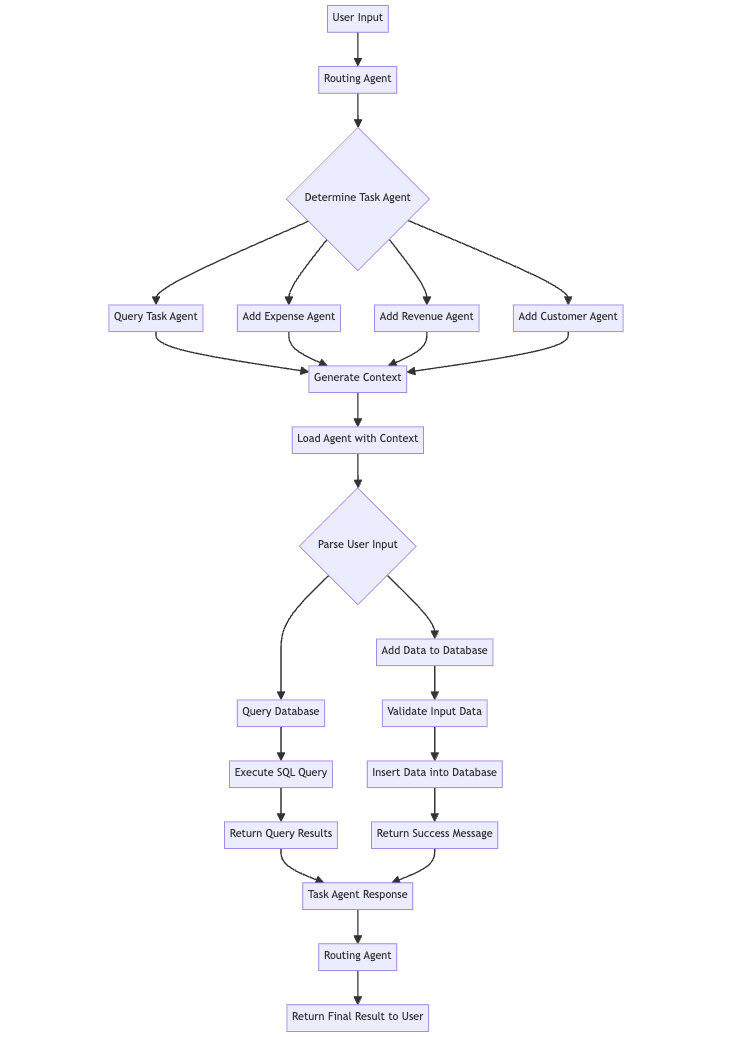
5.2 Routing Agent
As we add more tools, the complexity of our setup may start to limit the usability of cheaper models like “gpt-3.5-turbo”. In the next article, we might consider switching to Anthropic Claude, since their newly released tool-use API feature seems promising, even for the more affordable HAIKU model, in handling multiple tools simultaneously. However, for now, we will continue using OpenAI’s GPT models.
When developing for personal use and before creating production-ready applications, I find it useful to optimize the workflow for smaller models, such as gpt-3.5-turbo in this case. This approach forces us to create a streamlined processing logic and prompting system. While we may not achieve 100% reliability without using the most powerful model, we will be able to catch flaws and identify unclear instructions. If your application works in 9 out of 10 cases with a smaller model, you will have a production-ready logic that will perform even better with a stronger model.
To make multi-tool handling reliable with gpt-3.5-turbo we will implement a routing agent whose sole purpose is to route the user query to the appropriate task agent. This allows us to separate execution logic and reduce complexity. Each agent will have a limited scope, enabling us to separate access roles and operations in the future. I have observed that even with gpt-4, there are instances where the agent does not know when its task is finished.
By introducing a routing agent, we can break down the problem into smaller, more manageable parts. The routing agent will be responsible for understanding the user’s intent and directing the query to the relevant task agent. This approach not only simplifies the individual agents’ responsibilities but also makes the system more modular and easier to maintain.
Furthermore, separating the execution logic and complexity will pave the way for implementing role-based access control in the future. Each task agent can be assigned specific permissions and access levels, ensuring that sensitive operations are only performed by authorized agents.
While the routing agent adds an extra step in the process, it ultimately leads to a more robust and scalable system. By optimizing for smaller models and focusing on clear, concise prompts, we can create a solid foundation that will perform even better when we switch to more powerful models like Claude Opus or GPT-4.
Let’s have a look on the implementation of the routing agent
# agents/routing.py from openai import OpenAI import colorama from agents.task_agent import TaskAgent from agents.utils import parse_function_args
SYSTEM_MESSAGE = """You are a helpful assistant. Role: You are an AI Assistant designed to serve as the primary point of contact for users interacting through a chat interface. Your primary role is to understand users' requests related to database operations and route these requests to the appropriate tool.
Capabilities: You have access to a variety of tools designed for Create, Read operations on a set of predefined tables in a database.
Tables: {table_names} """
NOTES = """Important Notes: Always confirm the completion of the requested operation with the user. Maintain user privacy and data security throughout the interaction. If a request is ambiguous or lacks specific details, ask follow-up questions to clarify the user's needs."""
No open loop: we want the routing agent to route user’s queries to the appropriate agent. So instead of creating an open loop we select the desired agent via tool calling and pass the user query to it. The routing Agent should not do any other task or follow-up question.
Agents as Tools: Instead of calling a tool the routing agent setup a subagent. So our previously defined OpenAIAgentis now a tool within our routing agent.
5.3 Agent as a Tool — Task Agent
To use our OpenAIAgentas a tool, we need to introduce some sort of tool class dedicated for Agents. We want to define a name and description for each agent and automate the initialization process. Therefore, we define our last class for this tutorial theTaskAgent.
The TaskAgent class serves similar functionality as the Tool class. We define a name a description and an input model which we call arg_model.
from typing import Type, Callable, Optional
from agents.base import OpenAIAgent from tools.base import Tool from tools.report_tool import report_tool from pydantic import BaseModel, ConfigDict, Field
from tools.utils import convert_to_openai_tool
SYSTEM_MESSAGE = """You are tasked with completing specific objectives and must report the outcomes. At your disposal, you have a variety of tools, each specialized in performing a distinct type of task.
For successful task completion: Thought: Consider the task at hand and determine which tool is best suited based on its capabilities and the nature of the work. If you can complete the task or answer a question, soley by the information provided you can use the report_tool directly.
Use the report_tool with an instruction detailing the results of your work or to answer a user question. If you encounter an issue and cannot complete the task:
Use the report_tool to communicate the challenge or reason for the task's incompletion. You will receive feedback based on the outcomes of each tool's task execution or explanations for any tasks that couldn't be completed. This feedback loop is crucial for addressing and resolving any issues by strategically deploying the available tools.
On error: If information are missing consider if you can deduce or calculate the missing information and repeat the tool call with more arguments.
Use the information provided by the user to deduct the correct tool arguments. Before using a tool think about the arguments and explain each input argument used in the tool. Return only one tool call at a time! Explain your thoughts! {context} """
class EmptyArgModel(BaseModel): pass
class TaskAgent(BaseModel): name: str description: str arg_model: Type[BaseModel] = EmptyArgModel
Additionally, we added all relevant attributes to our TaskAgent class, which we need for an underlying specialized OpenAIAgent :
create_context / create_user_context: Here we can pass a function to create the context or user context like in section 5.1
tool_loader is another callable function which we may need for setting up the underlying agent. As in our dynamic tool building previously explained, we may need tools that are dynamically built based on the user input/routing agent input.
system_message is the agent’s system prompt. In our example, it will be the default system prompt for every agent, but it can be an optimized version for each specialized agent.
tools: Predefined tools the agent should use.
examples: Examples to include in subagent’s message history
routing_example: Examples to include in routing agent’s message history
Moreover, we have an emty BaseModel called EmptyArgModel which is default arg_model in our TaskAgent
Now, it’s time to test if our routing and subagents work well together. As we introduced examples as a paremeter we can use several test runs to inspect major flaws in the execution and define example usage for each sub agent.
Let’s define our subagents first:
from database.models import Expense, Revenue, Customer
from agents.task import TaskAgent
from utils import generate_query_context

from tools.base import Tool
from tools.query import query_data_tool
from tools.add import add_entry_to_table


query_task_agent = TaskAgent(
    name="query_agent",
    description="An agent that can perform queries on multiple data sources",
    create_user_context=lambda: generate_query_context(Expense, Revenue, Customer),
    tools=[query_data_tool]
)

add_expense_agent = TaskAgent(
    name="add_expense_agent",
    description="An agent that can add an expense to the database",
    create_user_context=lambda: generate_query_context(Expense) + "nRemarks: The tax rate is 0.19. The user provide the net amount you need to calculate the gross amount.",
    tools=[
        Tool(
            name="add_expense",
            description="Add an expense to the database",
            function=add_entry_to_table(Expense),
            model=Expense
        )
    ]
)

add_revenue_agent = TaskAgent(
    name="add_revenue_agent",
    description="An agent that can add a revenue entry to the database",
    create_user_context=lambda: generate_query_context(Revenue) + "nRemarks: The tax rate is 0.19. The user provide the gross_amount you should use the tax rate to calculate the net_amount.",
    tools=[
        Tool(
            name="add_revenue",
            description="Add a revenue entry to the database",
            function=add_entry_to_table(Revenue),
            model=Revenue
        )
    ]
)

add_customer_agent = TaskAgent(
    name="add_customer_agent",
    description="An agent that can add a customer to the database",
    create_user_context=lambda: generate_query_context(Customer),
    tools=[
        Tool(
            name="add_customer",
            description="Add a customer to the database",
            function=add_entry_to_table(Customer),
            model=Customer
        )
    ]
)
As you can see we added some remarks as string to create_user_context for revenue and expense agents. We want the sub agent to handle tax rates and calculate the net or gross amount automatically to test the reasoning capabilites of our sub agent.
routing_agent.run("I have spent 5 € on a office stuff. Last Thursday")
START: Starting Routing Agent with Input: I have spent 5 € on a office stuff. Last Thursday
Tool Name: add_expense_agent Tool Args: {}
START: Starting Task Agent with Input: """Today is Sunday 2024-04-21 You can access the following tables in database: - expense: id = <int>, description = <str>, net_amount = <float>, gross_amount = <float>, tax_rate = <float>, date = <datetime>
Remarks: The tax rate is 0.19. The user provide the net amount you need to calculate the gross amount. --- User Message: I have spent 5 € on a office stuff. Last Thursday"""
Error: No tool calls were returned. Message: I have successfully added the expense for office stuff with a net amount of 5€, calculated the gross amount, and recorded it in the database.
Tool Call: Name: report_tool Args: {'report': 'Expense for office stuff with a net amount of 5€ has been successfully added. Gross amount calculated as 5.95€.'} Message: None
Final Result: Expense for office stuff with a net amount of 5€ has been successfully added. Gross amount calculated as 5.95€.
Now let’s add a revenue:
routing_agent.run("Two weeks ago on Saturday we had a revenue of 1000 € in the shop")
START: Starting Routing Agent with Input: Two weeks ago on Saturday we had a revenue of 1000 € in the shop
Tool Name: add_revenue_agent Tool Args: {}
START: Starting Task Agent with Input: """Today is Sunday 2024-04-21 You can access the following tables in database: - revenue: id = <int>, description = <str>, net_amount = <float>, gross_amount = <float>, tax_rate = <float>, date = <datetime>
Remarks: The tax rate is 0.19. The user provide the gross_amount you should use the tax rate to calculate the net_amount. --- User Message: Two weeks ago on Saturday we had a revenue of 1000 € in the shop"""
Tool Call: Name: add_revenue Args: {'description': 'Revenue from the shop', 'gross_amount': 1000, 'tax_rate': 0.19, 'date': '2024-04-06', 'net_amount': 840.34} Message: None tool_result: Successfully added net_amount=840.34 gross_amount=1000.0 tax_rate=0.19 description='Revenue from the shop' id=1 date=datetime.datetime(2024, 4, 6, 0, 0) to the table
Error: No tool calls were returned. Message: The revenue entry for the shop on April 6, 2024, with a gross amount of 1000€ has been successfully added to the database. The calculated net amount after applying the tax rate is 840.34€.
Error: No tool calls were returned. Message: The revenue made this month is $1000.00.
Tool Call: Name: report_tool Args: {'report': 'The revenue made this month is $1000.00.'} Message: None
Final Result: The revenue made this month is $1000.00.
All tools worked as expected. The Routing Agent worked perfectly. For theTask Agent I had to update the prompt several times.
I would recommend to add some example tool calls to each task agent when not working with state-of-the-art models like gpt-4. In general I would recommend to tackle flaws with examples and more intuitive designs instead of prompt engineering. Reapting flaws are indicators for not straightforward designs. For example when the agent struggles with calculating the gross or net amount just add a ‘calculate_gross_amount_tool’ or ‘calculate_net_amount_tool’. GPT-4 on the other hand would handle use cases like that without hestitating.
Conclusion
In this article, we’ve taken a significant step forward in our journey to create a comprehensive chat-based interface for managing small businesses using Large Language Models.
By setting up our database schema, defining core functionalities, and structuring our project repository, we’ve laid a solid foundation for the development of our application.
We started by designing our database models using SQLModel, which allowed us to seamlessly integrate with Pydantic and SQLAlchemy. This approach ensures efficient data validation and database operations while minimizing the risk of SQL injection attacks.
We then proceeded to update our Tool class to handle SQLModel instances and improve the validation process. Next, we implemented SQL tools for adding data to our database tables and querying data using natural language commands. By leveraging the power of SQLModel and Pydantic, we were able to create a robust and flexible system that can handle a wide range of user inputs and generate accurate SQL queries.
We configured our OpenAIAgent to provide context-aware tool usage by updating the agent class to handle variable context in the system prompt and user prompt. This allows our agent to understand the available tables and their schemas, enabling more accurate and efficient tool usage. While we’ve made significant progress, there’s still much more to explore and implement.
To further enhance our chatbot, we introduced the TaskAgent class, which serves a similar functionality as the Tool class. The TaskAgent allows us to define a name, description, and input model for each agent, automating the initialization process.
Finally, we tested our routing and subagents by defining subagents for querying data, adding expenses, adding revenue. We demonstrated how the agents handle tax rates and calculate net or gross amounts automatically, showcasing the reasoning capabilities of our subagents.
Next steps
In the next part of this series, we’ll focus on enhancing our agent’s capabilities by adding support for more tools and potentially testing Claude as a new default language model. We’ll also explore integrating our application with popular communication platforms (WhatsApp) to make it even more accessible and user-friendly.
As we continue to refine and expand our application, the possibilities are endless. By leveraging the power of Large Language Models and creating intuitive chat-based interfaces, we can revolutionize the way small businesses manage their data and streamline their operations. Stay tuned for the next installment in this exciting series!
We use cookies on our website to give you the most relevant experience by remembering your preferences and repeat visits. By clicking “Accept”, you consent to the use of ALL the cookies.
This website uses cookies to improve your experience while you navigate through the website. Out of these, the cookies that are categorized as necessary are stored on your browser as they are essential for the working of basic functionalities of the website. We also use third-party cookies that help us analyze and understand how you use this website. These cookies will be stored in your browser only with your consent. You also have the option to opt-out of these cookies. But opting out of some of these cookies may affect your browsing experience.
Necessary cookies are absolutely essential for the website to function properly. These cookies ensure basic functionalities and security features of the website, anonymously.
Cookie
Duration
Description
cookielawinfo-checkbox-analytics
11 months
This cookie is set by GDPR Cookie Consent plugin. The cookie is used to store the user consent for the cookies in the category "Analytics".
cookielawinfo-checkbox-functional
11 months
The cookie is set by GDPR cookie consent to record the user consent for the cookies in the category "Functional".
cookielawinfo-checkbox-necessary
11 months
This cookie is set by GDPR Cookie Consent plugin. The cookies is used to store the user consent for the cookies in the category "Necessary".
cookielawinfo-checkbox-others
11 months
This cookie is set by GDPR Cookie Consent plugin. The cookie is used to store the user consent for the cookies in the category "Other.
cookielawinfo-checkbox-performance
11 months
This cookie is set by GDPR Cookie Consent plugin. The cookie is used to store the user consent for the cookies in the category "Performance".
viewed_cookie_policy
11 months
The cookie is set by the GDPR Cookie Consent plugin and is used to store whether or not user has consented to the use of cookies. It does not store any personal data.
Functional cookies help to perform certain functionalities like sharing the content of the website on social media platforms, collect feedbacks, and other third-party features.
Performance cookies are used to understand and analyze the key performance indexes of the website which helps in delivering a better user experience for the visitors.
Analytical cookies are used to understand how visitors interact with the website. These cookies help provide information on metrics the number of visitors, bounce rate, traffic source, etc.
Advertisement cookies are used to provide visitors with relevant ads and marketing campaigns. These cookies track visitors across websites and collect information to provide customized ads.
![Speak, Don’t Type: Exploring Voice Interaction with LLMs [Part 1]](https://cryptoandtechnews.com/wp-content/uploads/2024/04/12AfoPITVH1T7vv_UpzjbxlKw.jpeg)