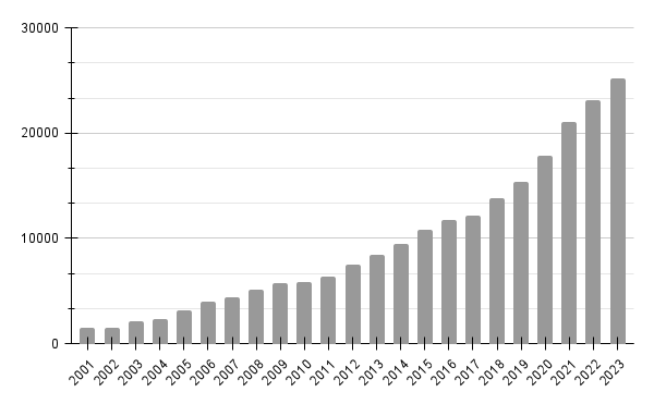
Choosing between frequentist and Bayesian approaches is the great debate of the last century, with a recent surge in Bayesian adoption in the sciences.
Number of articles referring Bayesian statistics in sciencedirect.com (April 2024) — Graph by the author
What’s the difference?
The philosophical difference is actually quite subtle, where some propose that the great bayesian critic, Fisher, was himself a bayesian in some regard. While there are countless articles that delve into formulaic differences, what are the practical benefits? What does Bayesian analysis offer to the lay data scientist that the vast plethora of highly-adopted frequentist methods do not already? This article aims to give a practical introduction to the motivation, formulation, and application of Bayesian methods. Let’s dive in.
Prior Beliefs
While frequentists deal with describing the exact distributions of any data, the bayesian viewpoint is more subjective. Subjectivity and statistics?! Yes, it’s actually compatible.
Let’s start with something simple, like a coin flip. Suppose you flip a coin 10 times, and get heads 7 times. What is the probability of heads?
P(heads) = 7/10 (0.7)?
Obviously, here we are riddled with low sample size. In a Bayesian POV however, we are allowed to encode our beliefs directly, asserting that if the coin is fair, the chance of heads or tails must be equal i.e. 1/2. While in this example the choice seems pretty obvious, the debate is more nuanced when we get to more complex, less obvious phenomenon.
Yet, this simple example is a powerful starting point, highlighting both the greatest benefit and shortcoming of Bayesian analysis:
Benefit: Dealing with a lack of data. Suppose you are modeling spread of an infection in a country where data collection is scarce. Will you use the low amount of data to derive all your insights? Or would you want to factor-in commonly seen patterns from similar countries into your model i.e. informed prior beliefs. Although the choice is clear, it leads directly to the shortcoming.
Shortcoming: the prior belief is hard to formulate. For example, if the coin is not actually fair, it would be wrong to assume that P (heads) = 0.5, and there is almost no way to find true P (heads) without a long run experiment. In this case, assuming P (heads) = 0.5 would actually be detrimental to finding the truth. Yet every statistical model (frequentist or Bayesian) must make assumptions at some level, and the ‘statistical inferences’ in the human mind are actually a lot like bayesian inference i.e. constructing prior belief systems that factor into our decisions in every new situation. Additionally, formulating wrong prior beliefs is often not a death sentence from a modeling perspective either, if we can learn from enough data (more on this in later articles).
Bayes’ Rule
So what does all this look like mathematically? Bayes’ rule lays the groundwork. Let’s suppose we have a parameter θ that defines some model which could describe our data (eg. θ could represent the mean, variance, slope w.r.t covariate, etc.). Bayes’ rule states that
P (θ = t|data) represents the conditional probability that θ is equal to t, given our data (a.k.a the posterior).
Conversely, P (data|θ) represents the probability of observing our data, if θ = t (a.k.a the ‘likelihood’).
Finally, P (θ=t) is simply the probability that θ takes the value t (the infamous ‘prior’).
So what’s this mysterious t? It can take many possible values, depending on what θ means. In fact, you want to try a lot of values, and check the likelihood of your data for each. This is a key step, and you really really hope that you checked the best possible values for θ i.e. those which cover the maximum likelihood area of seeing your data (global minima, for those who care).
And that’s the crux of everything Bayesian inference does!
Form a prior belief for possible values of θ,
Scale it with the likelihood at each θ value, given the observed data, and
Return the computed result i.e. the posterior, which tells you the probability of each tested θ value.
Graphically, this looks something like:
Prior (left) scaled with the likelihood (middle) forms the posterior (right) (figures adapted from Andrew Gelmans Book). Here, θ encodes the east-west location coordinate of a plane. The prior belief is that the plane is more towards the east than west. The data challenges the prior and the posterior thus lies somehwere in the middle. [image using data generated by author]
Which highlights the next big advantages of Bayesian stats-
We have an idea of the entire shape of θ’s distribution (eg, how wide is the peak, how heavy are the tails, etc.) which can enable more robust inferences. Why? Simply because we can not only better understand but also quantify the uncertainty (as compared to a traditional point estimate with standard deviation).
Since the process is iterative, we can constantly update our beliefs (estimates) as more data flows into our model, making it much easier to build fully online models.
Easy enough! But not quite…
This process involves a lot of computations, where you have to calculate the likelihood for each possible value of θ. Okay, maybe this is easy if suppose θ lies in a small range like [0,1]. We can just use the brute-force grid method, testing values at discrete intervals (10, 0.1 intervals or 100, 0.01 intervals, or more… you get the idea) to map the entire space with the desired resolution.
But what if the space is huge, and god forbid additional parameters are involved, like in any real-life modeling scenario?
Now we have to test not only the possible parameter values but also all their possible combinations i.e. the solution space expands exponentially, rendering a grid search computationally infeasible. Luckily, physicists have worked on the problem of efficient sampling, and advanced algorithms exist today (eg. Metropolis-Hastings MCMC, Variational Inference) that are able to quickly explore high dimensional spaces of parameters and find convex points. You don’t have to code these complex algorithms yourself either, probabilistic computing languages like PyMC or STAN make the process highly streamlined and intuitive.
STAN
STAN is my favorite as it allows interfacing with more common data science languages like Python, R, Julia, MATLAB etc. aiding adoption. STAN relies on state-of-the-art Hamiltonian Monte Carlo sampling techniques that virtually guarantee reasonably-timed convergence for well specified models. In my next article, I will cover how to get started with STAN for simple as well as not-no-simple regression models, with a full python code walkthrough. I will also cover the full Bayesian modeling workflow, which involves model specification, fitting, visualization, comparison, and interpretation.
The Landscape of Emerging AI Agent Architectures for Reasoning, Planning, and Tool Calling: A Survey
Image by Author
My team and I (Sandi Besen, Tula Masterman, Mason Sawtell, and Alex Chao) recently published a survey research paper that offers a comprehensive look at the current state of AI agent architectures. As co-authors of this work, we set out to uncover the key design elements that enable these autonomous systems to effectively execute complex goals.
This paper serves as a resource for researchers, developers, and anyone interested in staying updated on the cutting-edge progress in the field of AI agent technologies.
Since the launch of ChatGPT, the initial wave of generative AI applications has largely revolved around chatbots that utilize the Retrieval Augmented Generation (RAG) pattern to respond to user prompts. While there is ongoing work to enhance the robustness of these RAG-based systems, the research community is now exploring the next generation of AI applications — a common theme being the development of autonomous AI agents.
Agentic systems incorporate advanced capabilities like planning, iteration, and reflection, which leverage the model’s inherent reasoning abilities to accomplish tasks end-to-end. Paired with the ability to use tools, plugins, and function calls — agents are empowered to tackle a wider range of general-purpose work.
The Importance of Reasoning, Planning, and Effective Tool Calling for Agents
Reasoning is a foundational building block of the human mind. Without reasoning one would not be able to make decisions, solve problems, or refine plans when new information is learned — essentially misunderstanding the world around us. If agents don’t have strong reasoning skills then they might misunderstand their task, generate nonsensical answers, or fail to consider multi-step implications.
We find that most agent implementations contain a planning phase which invokes one of the following techniques to create a plan: task decomposition, multi-plan selection, external module-aided planning, reflection and refinement and memory-augmented planning [1].
Another benefit of utilizing an agent implementation over just a base language model is the agent’s ability to solve complex problems by calling tools. Tools can enable an agent to execute actions such as interacting with APIs, writing to third party applications, and more. Reasoning and tool calling are closely intertwined and effective tool calling has a dependency on adequate reasoning. Put simply, you can’t expect an agent with poor reasoning abilities to understand when is the appropriate time to call its tools.
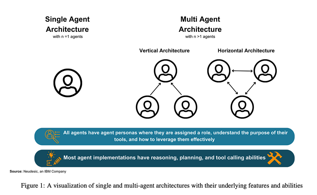
Single vs Multi Agent Architecture
Our findings emphasize that both single-agent and multi-agent architectures can be used to solve challenging tasks by employing reasoning and tool calling steps.
For single agent implementations, we find that successful goal execution is contingent upon proper planning and self-correction [1, 2, 3, 4]. Without the ability to self-evaluate and create effective plans, single agents may get stuck in an endless execution loop and never accomplish a given task or return a result that does not meet user expectations [2]. We find that single agent architectures are especially useful when the task requires straightforward function calling and does not need feedback from another agent.
However, we note that single agent patterns often struggle to complete a long sequence of sub tasks or tool calls [5, 6]. Multi-agent patterns can address the issues of parallel tasks and robustness since multiple agents within the architecture can work on individual subproblems. Many multi-agent patterns start by taking a complex problem and breaking it down into several smaller tasks. Then, each agent works independently on solving each task using their own independent set of tools.
Architectures involving multiple agents present an opportunity for intelligent labor division based on capabilities as well as valuable feedback from diverse agent personas. Numerous multi-agent architectures operate in stages where teams of agents are dynamically formed and reorganized for each planning, execution, and evaluation phase [7, 8, 9]. This reorganization yields superior outcomes because specialized agents are utilized for specific tasks and removed when no longer required. By matching agent roles and skills to the task at hand, agent teams can achieve greater accuracy and reduce the time needed to accomplish the goal. Crucial features of effective multi-agent architectures include clear leadership within agent teams, dynamic team construction, and efficient information sharing among team members to prevent important information from getting lost amidst superfluous communication.
Our research highlights notable single agent methods such as ReAct, RAISE, Reflexion, AutoGPT + P, LATS, and multi agent implementations such as DyLAN, AgentVerse, and MetaGPT, which are explained more in depth in the full text.
Our Key Findings
Single Agent Patterns:
Single agent patterns are generally best suited for tasks with a narrowly defined list of tools and where processes are well-defined. They don’t face poor feedback from other agents or distracting and unrelated chatter from other team members. However, single agents may get stuck in an execution loop and fail to make progress towards their goal if their reasoning and refinement capabilities aren’t robust.
Multi Agent Patterns:
Multi agent patterns are well-suited for tasks where feedback from multiple personas is beneficial in accomplishing the task. They are useful when parallelization across distinct tasks or workflows is required, allowing individual agents to proceed with their next steps without being hindered by the state of tasks handled by others.
Feedback and Human in the Loop
Language models tend to commit to an answer earlier in their response, which can cause a ‘snowball effect’ of increasing diversion from their goal state [10]. By implementing feedback, agents are much more likely to correct their course and reach their goal. Human oversight improves the immediate outcome by aligning the agent’s responses more closely with human expectations, yielding more reliable and trustworthy results [11, 8]. Agents can be susceptible to feedback from other agents, even if the feedback is not sound. This can lead the agent team to generate a faulty plan which diverts them from their objective [12].
Information Sharing and Communication
Multi-agent patterns have a greater tendency to get caught up in niceties and ask one another things like “how are you”, while single agent patterns tend to stay focused on the task at hand since there is no team dynamic to manage. This can be mitigated by robust prompting. In vertical architectures, agents can fail to send critical information to their supporting agents not realizing the other agents aren’t privy to necessary information to complete their task. This failure can lead to confusion in the team or hallucination in the results. One approach to address this issue is to explicitly include information about access rights in the system prompt so that the agents have contextually appropriate interactions.
Impact of Role Definition and Dynamic Teams
Clear role definition is critical for both single and multi-agent architectures. Role definition ensures that the agents understands their assigned role, stay focused on the provided task, execute the proper tools, and minimizes hallucination of other capabilities. Establishing a clear group leader improves the overall performance of multi-agent teams by streamlining task assignment. Dynamic teams where agents are brought in and out of the system based on need have also been shown to be effective. This ensures that all agents participating in the tasks are strong contributors.
Summary of Key Insights
The key insights discussed suggest that the best agent architecture varies based on use case. Regardless of the architecture selected, the best performing agent systems tend to incorporate at least one of the following approaches: well defined system prompts, clear leadership and task division, dedicated reasoning / planning- execution — evaluation phases, dynamic team structures, human or agentic feedback, and intelligent message filtering. Architectures that leverage these techniques are more effective across a variety of benchmarks and problem types.
Conclusion
Our meta-analysis aims to provide a holistic understanding of the current AI agent landscape and offer insight for those building with existing agent architectures or developing custom agent architectures. There are notable limitations and areas for future improvement in the design and development of autonomous AI agents such as a lack of comprehensive agent benchmarks, real world applicability, and the mitigation of harmful language model biases. These areas will need to be addressed in the near-term to enable reliable agents.
Note: The opinions expressed both in this article and paper are solely those of the authors and do not necessarily reflect the views or policies of their respective employers.
If you still have questions or think that something needs to be further clarified? Drop me a DM on Linkedin! I‘m always eager to engage in food for thought and iterate on my work.
References
[1] Timo Birr et al. AutoGPT+P: Affordance-based Task Planning with Large Language Models. arXiv:2402.10778 [cs] version: 1. Feb. 2024. URL: http://arxiv.org/abs/2402.10778.
[2] Shunyu Yao et al. ReAct: Synergizing Reasoning and Acting in Language Models. arXiv:2210.03629 [cs]. Mar. 2023. URL: http://arxiv.org/abs/2210.03629.
[3] Na Liu et al. From LLM to Conversational Agent: A Memory Enhanced Architecture with Fine-Tuning of Large Language Models. arXiv:2401.02777 [cs]. Jan. 2024. URL: http://arxiv.org/abs/2401.02777.
[4] Noah Shinn et al. Reflexion: Language Agents with Verbal Reinforcement Learning. arXiv:2303.11366 [cs]. Oct. 2023. URL: http://arxiv.org/abs/2303.11366.
[5]Zhengliang Shi et al. Learning to Use Tools via Cooperative and Interactive Agents. arXiv:2403.03031 [cs]. Mar. 2024. URL: http://arxiv.org/abs/2403.03031.
[6] Silin Gao et al. Efficient Tool Use with Chain-of-Abstraction Reasoning. arXiv:2401.17464 [cs]. Feb. 2024. URL: http://arxiv.org/abs/2401.17464
[7] Weize Chen et al. AgentVerse: Facilitating Multi-Agent Collaboration and Exploring Emergent Behaviors. arXiv:2308.10848 [cs]. Oct. 2023. URL: http://arxiv.org/abs/2308.10848.
[8] Xudong Guo et al. Embodied LLM Agents Learn to Cooperate in Organized Teams. 2024. arXiv: 2403.12482 [cs.AI].
[9] Zijun Liu et al. Dynamic LLM-Agent Network: An LLM-agent Collaboration Framework with Agent Team Optimization. 2023. arXiv: 2310.02170 [cs.CL].
[10] Muru Zhang et al. How Language Model Hallucinations Can Snowball. arXiv:2305.13534 [cs]. May 2023. URL: http://arxiv.org/abs/2305.13534.
[11] Xueyang Feng et al. Large Language Model-based Human-Agent Collaboration for Complex Task Solving. 2024. arXiv: 2402.12914 [cs.CL].
[12] Weize Chen et al. AgentVerse: Facilitating Multi-Agent Collaboration and Exploring Emergent Behaviors. arXiv:2308.10848 [cs]. Oct. 2023. URL: http://arxiv.org/abs/2308.10848.
A tutorial to demonstrate how to use Burr, using simple OpenAI client calls to GPT4, and FastAPI to create a custom email assistant agent.
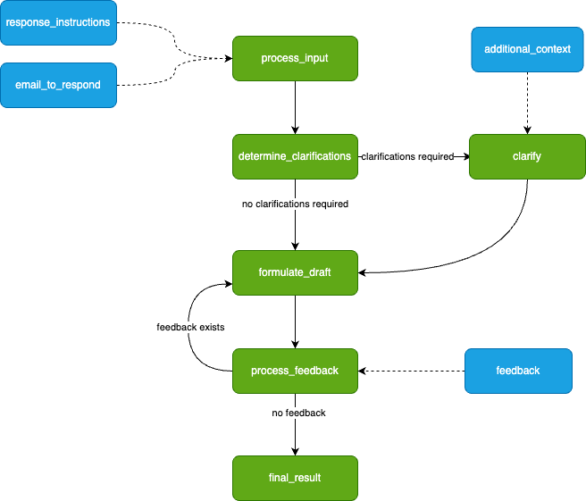
The control flow of the agent application we’ll create. Image by author.
In this tutorial, I will demonstrate how to use Burr, an open source framework (disclosure: I helped create it), using simple OpenAI client calls to GPT4, and FastAPI to create a custom email assistant agent. We’ll describe the challenge one faces and then how you can solve for them. For the application frontend we provide a reference implementation but won’t dive into details for it.
Why are interactive agents applications a challenge?
LLMs rarely achieve complex goals on their own, and almost never on the first try. While it is in vogue to claim that ChatGPT given an internet connection can solve the world’s problems, the majority of high-value tools we’ve encountered use a blend of AI ingenuity and human guidance. This is part of the general move towards building building agents — an approach where the AI makes decisions from information it receives — this could be information it queries, information a user provides, or information another LLM gives it.
A simple example of this is a tool to help you draft a response to an email. You put the email and your response goals, and it writes the response for you. At a minimum, you’ll want to provide feedback so it can adjust the response. Furthermore, you will want it to give a chance to ask clarifying questions (an overly confident yet incorrect chatbot helps no one).
In designing this interaction, your system will, inevitably, become a back-and-forth between user/LLM control. In addition to the standard challenges around AI applications (unreliable APIs, stochastic implementations, etc…), you will face a suite of new problems, including:
Logically modeling a set of interaction points/flows
Persisting the state so the user can pick up the interaction/application from where it left off
Monitoring the decisions the LLM made (E.G. whether to ask the user questions or not)
And so on… In this post we’re going to walk through how to approach solving these — we’ll use the Burr library as well as FastAPI to build a web service to address these challenges in an extensible, modular manner; so you can then use this as a blue print for your own agent assistant needs.
The Tools
Burr
Burr is a lightweight python library you use to build applications as state machines. You construct your application out of a series of actions (these can be either decorated functions or objects), which declare inputs from state, as well as inputs from the user. These specify custom logic (delegating to any framework), as well as instructions on how to update state. State is immutable, which allows you to inspect it at any given point. Burr handles orchestration, monitoring and persistence.
@action(reads=["counter"], writes=["counter"])
def count(state: State) -> Tuple[dict, State]:
    current = state["counter"] + 1
    result = {"counter": current}
    return result, state.update(counter=counter)
Note that the action above has two returns — the results (the counter), and the new, modified state (with the counter field incremented).
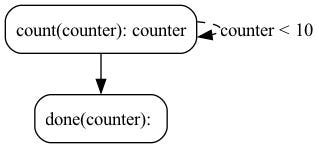
You run your Burr actions as part of an application — this allows you to string them together with a series of (optionally) conditional transitions from action to action.
from burr.core import ApplicationBuilder, default, expr
app = (
    ApplicationBuilder()
    .with_state(counter=0) # initialize the count to zero
    .with_actions(
        count=count,
        done=done # implementation left out above
    ).with_transitions(
        ("count", "count", expr("counter < 10")), # Keep counting if the counter is less than 10
        ("count", "done", default) # Otherwise, we're done
    ).with_entrypoint("count") # we have to start somewhere
    .build()
)
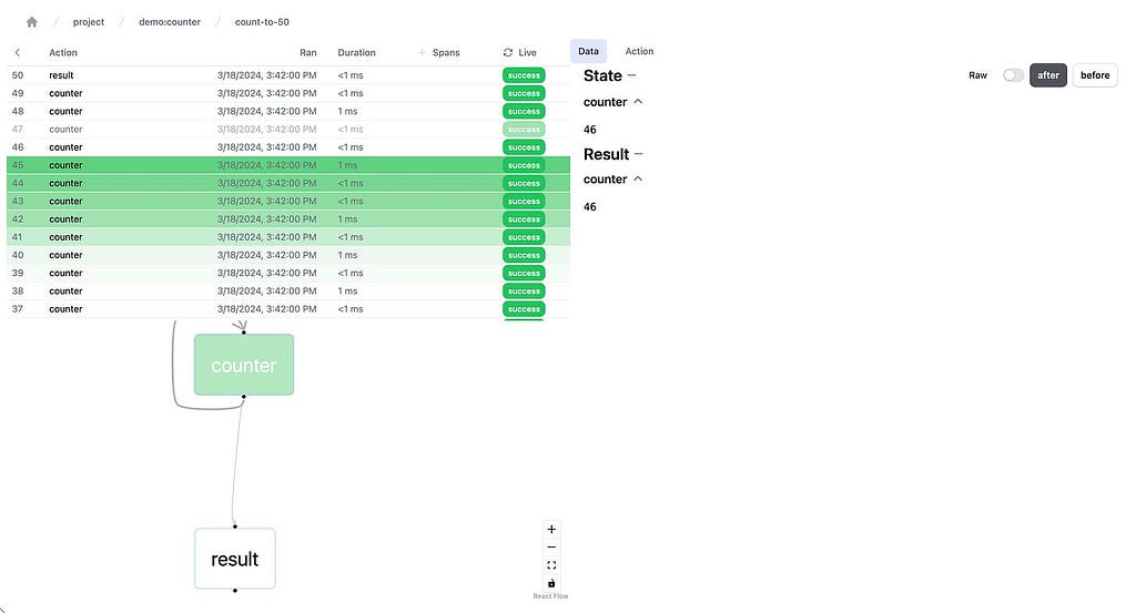
Burr comes with a user-interface that enables monitoring/telemetry, as well as hooks to persist state/execute arbitrary code during execution.
You can visualize this as a flow chart, i.e. graph / state machine:
Image of our application as produced by Burr. Image by author.
And monitor it using the local telemetry debugger:
Burr comes with a UI — this is what it looks like when inspecting a run of our counter example. Image by author.
While we showed the (very simple) counter example above, Burr is more commonly used for building chatbots/agents (we’ll be going over an example in this post).
FastAPI
FastAPI is a framework that lets you expose python functions in a REST API. It has a simple interface — you write your functions then decorate them, and run your script — turning it into a server with self-documenting endpoints through OpenAPI.
@app.get("/items/{item_id}") def read_item(item_id: int, q: Union[str, None] = None): """A very simpler example of an endpoint that takes in arguments.""" return {"item_id": item_id, "q": q}
FastAPI is easy to deploy on any cloud provider — it is infrastructure-agnostic and can generally scale horizontally (so long as consideration into state management is done). See this page for more information.
React (or any frontend framework)
You can use any frontend framework you want — react-based tooling, however, has a natural advantage as it models everything as a function of state, which can map 1:1 with the concept in Burr. In the demo app we use react, react-query, and tailwind, but we’ll be skipping over this largely (it is not central to the purpose of the post).
Building
Let’s dig a bit more into the conceptual model. At a high-level, our email assistant will do the following:
Accept an email + instructions to respond
Come up with a set of clarifying questions (if the LLM deems it required)
Generates a draft using the answer to those questions
Accept feedback to that draft and generates another one, repeating until the user is happy
Return the final draft (done)
Modeling Control Flow
As Burr requires you to build a control flow from actions and transitions, we can initially model this as a simple flowchart.
What our application will look like. Image by author.
We drafted this before actually writing any code — you will see it transforms to code naturally.
The green nodes represent actions (these take state in and modify it), and the blue nodes represent inputs (these are points at which the app has to pause and ask the user for information). Note that there is a loop (formulate_draft ⇔process_feedback) — we iterate on feedback until we’re happy with the results.
This diagram is simply a stylized version of what Burr shows you — the modeling is meant to be close to the actual code. We have not displayed state information (the data the steps take in/return), but we’ll need to track the following (that may or may not be populated at any given point) so we can make decisions about what to do next:
The initial inputs: {email_to_respond: str, response_instructions: str}
The questions the LLM asks and the user responses (if any):{clarifications: list[str], response_instructions: list[str]}
The list of drafts + feedback: {drafts: list[str], feedback_history: list[str]}
The final result: {final_result: str}
Implementing/Testing
Looking at the requirements above, we can build a straightforward burr application since we can very closely match our code with our diagram above. Let’s take a look at the determine_clarifications step, for example:
@action( reads=["response_instructions", "incoming_email"], writes=["clarification_questions"] ) def determine_clarifications(state: State) -> Tuple[dict, State]: """Determines if the response instructions require clarification."""
result = client.chat.completions.create( model="gpt-4", messages=[ { "role": "system", "content": ("You are a chatbot that has the task of " "generating responses to an email on behalf " "of a user. "), }, { "role": "user", "content": ( f"The email you are to respond to is: {incoming_email}." # ... left out, see link above "The questions, joined by newlines, must be the only " "text you return. If you do not need clarification, " "return an empty string." ), }, ], ) content = result.choices[0].message.content all_questions = content.split("n") if content else [] return {"clarification_questions": all_questions}, state.update( clarification_questions=all_questions)
Note that this uses simple OpenAI calls — you can replace this with Langchain, LlamaIndex, Hamilton (or something else) if you prefer more abstraction, and delegate to whatever LLM you like to use. And, you should probably use something a little more concrete (E.G. instructor) to guarantee output shape.
To tie these together, we put them into the application builder — this allows us to set conditional transitions (e.g. len(clarification_questions>0) and therefore connect actions, recreating the diagram above.
To iterate on this, we used a jupyter notebook. Running our application is simple — all you do is call the .run() method on the Application, with the right halting conditions. We’ll want it to halt before any action that requires user input (clarify_instructions and process_feedback), and after final_result. We can then run it in a while loop, asking for user input and feeding it back to the state machine:
def request_answers(questions):
    """Requests answers from the user for the questions the LLM has"""
    answers = []
    print("The email assistant wants more information:n")
    for question in questions:
        answers.append(input(question))
    return answers

def request_feedback(draft):
    """Requests feedback from the user for a draft"""
    print(
        f"here's a draft!: n {draft} n n What feedback do you have?",
    )
    return input("Write feedback or leave blank to continue (if you're happy)")
inputs = {
    "email_to_respond" : EMAIL,
    "response_instructions" : INSTRUCTIONS
}

# in our notebook cell:
while True:
    action, result, state = app.run(
        halt_before=["clarify_instructions", "process_feedback"],
        halt_after=["final_result"],
        inputs=inputs
    )
    if action.name == "clarify_instructions":
        questions = state["clarification_questions"]
        answers = request_answers(questions)
        inputs = {
            "clarification_inputs" : answers
        }
    if action.name == "process_feedback":
        feedback = request_feedback(state["current_draft"])
        inputs = {"feedback" : feedback}
    if action.name == "final_result":
        print("final result is:", state["current_draft"])
        break
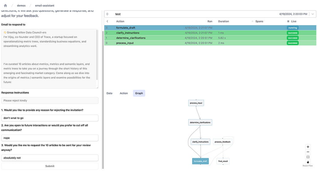
You can then use the Burr UI to monitor your application as it runs!
Example of using the Burr UI (with the email app UI) and then seeing it’s execution. Image by author.
Persistence
We’re going to persist our results to an SQLite server (although as you’ll see later on this is customizable). To do this, we need to add a few lines to the ApplicationBuilder.
app = ( ApplicationBuilder(). ... # the code we had above .initialize( initializer=state_persister, resume_at_next_action=True, default_state={"chat_history" : []}, default_entrypoint="process_input" ) .with_identifiers(app_id=app_id) .build() )
This ensures that every email draft we create will be saved and can be loaded at every step. When you want to resume a prior draft of an email, all you have to do is rerun the code and it will start where it left off.
Integrating in a web server
To expose this in a web server we’ll be using FastAPI to create endpoints and Pydantic to represent types. Before we get into the details, we’ll note that Burr naturally provides an application_id (either generated or specified) for every instance of an application. In this case the application_id would correspond to a particular email draft. This allows us to uniquely access it, query from the db, etc… It also allows for a partition key (E.G. user_id) so you can add additional indexing in your database. We center the API around inputs/outputs
Endpoints
We will construct the following endpoints:
POST /create: This will create a new application and return the ID
PUT /initialize_draft/{id}/: This calls out to process_input, passing in the email and instructions
PUT /clarify_instructions/{id}: This will give answers back to the LLM
PUT /process_feedback/{id}: This will give feedback back to the LLM
GET /{id}/state: This will return the current state of the application
The GET endpoint allows us to get the current state of the application — this enables the user to reload if they quit the browser/get distracted. Each of these endpoints will return the full state of the application, which can be rendered on the frontend. Furthermore, it will indicate the next API endpoint we call, which allows the UI to render the appropriate form and submit to the right endpoint.
Using FastAPI + Pydantic, this becomes very simple to implement. First, let’s add a utility to get the application object. This will use a cached version or instantiate it:
All this does is call our function application in email_assistant that recreates the application. We have not included the create function here, but it calls out to the same API.
Data Model
Let’s then define a Pydantic model to represent the state, and the app object in FastAPI:
class EmailAssistantState(pydantic.BaseModel):
    app_id: str
    email_to_respond: Optional[str]
    response_instructions: Optional[str]
    questions: Optional[List[str]]
    answers: Optional[List[str]]
    drafts: List[str]
    feedback_history: List[str]
    final_draft: Optional[str]
    # This stores the next step, which tells the frontend which ones to call
    next_step: Literal[
        "process_input", "clarify_instructions",
        "process_feedback", None]

@staticmethod
    def from_app(app: Application):
        # implementation left out, call app.state and translate to
        # pydantic model we can use `app.get_next_action()` to get
        #the next step and return it to the user
        ...
Note that every endpoint will return this same pydantic model!
Endpoints
Given that each endpoint returns the same thing (a representation of the current state as well as the next step to execute), they all look the same. We can first implement a generic run_throughfunction, which will progress our state machine forward, and return the state.
This represents a simple but powerful architecture. We can continue calling these endpoints until we’re at a “terminal” state, at which point we can always ask for the state. If we decide to add more input steps, we can modify the state machine and add more input steps. We are not required to hold state in the app (it is all delegated to Burr’s persistence), so we can easily load up from any given point, allowing the user to wait for seconds, minutes, hours, or even days before continuing.
As the frontend simply renders based on the current state and the next step, it will always be correct, and the user can always pick up where they left off. With Burr’s telemetry capabilities you can debug any state-related issues, ensuring a smooth user experience.
Adding a UI
Now that we have a set of endpoints, the UI is simple. In fact, it mirrors the API almost exactly. We won’t dig into this too much, but the high-level is that you’ll want the following capabilities:
Render the current state (show the history, latest draft)
Include a form for the next action’s inputs (provide feedback, answer clarifications)
Post the results to your FastAPI endpoints, pause for response, GOTO (1)
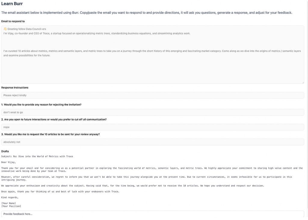
You can see the UI here. Here’s an example of it in action:
Note that there are many tools that make this easier/simpler to prototype, including chainlit, streamlit, etc… The backend API we built is amenable to interacting with them as well.
Additional Capabilities
Customizing Persistence
While we used the simple SQLLite persister, you can use any of the others that come with Burr or implement your own to match your schema/db infrastructure. To do this you implement the BaseStatePersister class, and add it in with the ApplicationBuilder, instead of the SQLLite persister we used above.
Additional Monitoring/Visibility
Using the Burr UI to monitor is not the only way. You can integrate your own by leveraging lifecycle hooks, enabling you to log data in a custom format to, say, datadog, langsmith, or langfuse.
Furthermore, you can leverage additional monitoring capabilities to track spans/traces, either logging them directly to the Burr UI or to any of the above providers. See the list of available hooks here.
Async/Streaming
While we kept the APIs we exposed synchronous for simplicity, Burr supports asynchronous execution as well. Burr also supports streaming responses for those who want to provide a more interactive UI/reduce time to first token.
So how does it do in practice?
As with any LLM application, the entire prompt matters. If you can provide the right guidance, the results are going to be better than if you don’t. Much like if you are going to instruct a human, more guidance is always better. That said, if you find yourself always correcting some aspect, then changing the base prompt is likely the best course of action. For example, using a single-shot or few-shot approach might be a good choice to try to help instruct the LLM as to what you’d like to see given your specific context.
Post Summary
In this post we discussed how to address some of the challenges around building human-in-the-loop agentic workflows. We ran through an example of making an email assistant using Burr to build and run it as a state machine, and FastAPI to run Burr in a web service. We finally showed how you can extend the tooling we used here for a variety of common production needs — e.g. monitoring & storage.
Additional Resources
Join Burr’s Discord for help or if you have questions!
Speaker diarization, an essential process in audio analysis, segments an audio file based on speaker identity. This post delves into integrating Hugging Face’s PyAnnote for speaker diarization with Amazon SageMaker asynchronous endpoints. We provide a comprehensive guide on how to deploy speaker segmentation and clustering solutions using SageMaker on the AWS Cloud.
Organizations across industries are using automatic text summarization to more efficiently handle vast amounts of information and make better decisions. In the financial sector, investment banks condense earnings reports down to key takeaways to rapidly analyze quarterly performance. Media companies use summarization to monitor news and social media so journalists can quickly write stories on […]
The fundamental principles of math that data scientists use in their day-to-day work may have been around for centuries, but that doesn’t mean we should approach the topic as if we only learn it once and then store away our knowledge in some dusty mental attic. Practical approaches, tools, and use cases evolve all the time—and with them comes the need to stay up-to-date.
This week, we’re thrilled to share a strong lineup of recent math and stats must-reads, covering a wide range of questions and applications. From leveraging (very) small datasets to presenting linear regressions in accessible, engaging ways, we’re sure you’ll find something new and useful to explore. Let’s dive in!
N-of-1 Trials and Analyzing Your Own Fitness Data The idea behind N-of-1 studies is that you can draw meaningful insights even when the data you’re using is based on input from a single person. It has far-reaching potential for designing individualized healthcare strategies, or, in the case of Merete Lutz’s fascinating project, establishing meaningful connections between alcohol consumption and sleep quality.
How Reliable Are Your Time Series Forecasts, Really? Making long-term predictions is easy; making accurate long-term predictions is, well, less so. Bradley Stephen Shaw recently shared a useful guide to help you determine the reliability horizon of your forecasts through the effective use of cross-validation, visualization, and statistical hypothesis testing.
Building a Math Application with LangChain Agents Despite the major strides LLMs have made in the past couple of years, math remains an area they struggle with. In her latest hands-on tutorial, Tahreem Rasul unpacks the challenges we face when we try to make these models execute mathematical and statistical operations, and outlines a solution for building an LLM-based math app using LangChain agents, OpenAI, and Chainlit.
A Proof of the Central Limit Theorem It’s always a joy to see an abstract concept take concrete shape and, along the way, become much more accessible and intuitive for learners. That’s precisely what Sachin Date accomplishes in his latest deep dive, which shows us the inner workings of the central limit theorem, “one of the most far-reaching and delightful theorems in statistical science,” through the example of… candy!
8 Plots for Explaining Linear Regression to a Layman Even if you, a professional data scientist or ML engineer, fully grasp the implications of your statistical analyses, chances are many of your colleagues and other stakeholders won’t. This is where strong visualizations can make a major difference, as Conor O’Sullivan demonstrates with eight different residual, weight, effect, and SHAP plots that explain linear regression models effectively.
Looking to branch out beyond math and stats this week? We hope so! Here are some of our best recent reads on other topics:
If you’re thinking of giving back to the community by contributing to an open-source project, don’t miss Mike Clayton’s terrific recap of his experience fixing bugs on the ever-popular Pandas library.
It’s no secret that the current job market is challenging for many data professionals. Erin Wilson’s visual recap of her recent journey offers a healthy dose of inspiration—and pragmatic insights—to support you on your job search.
Thank you for supporting the work of our authors! We love publishing articles from new authors, so if you’ve recently written an interesting project walkthrough, tutorial, or theoretical reflection on any of our core topics, don’t hesitate to share it with us.
How to improve your ML model with three lines of code
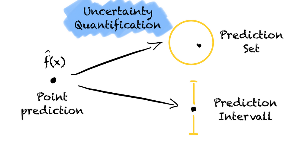
Turning a point prediction into a prediction region to quantify the model’s uncertainty to give us more information (Image by the author).
Prediction models are trained to predict well and give us point forecasts.
Let’s assume we want to buy a house. Before we do so, we want to verify that the advertised price of 400,000 € is reasonable. For this, we use a model that, based on the number of rooms, the size and the location of the house, predicts that the house is worth 500,232.12 €.
Should we buy this house? It seems like a good deal, doesn’t it? But would our decision be different if the model instead had predicted a price of 340,021.34 €? Probably, right?
Hence, should we trust the model when making the decision to buy this house? What is the probability that the house is worth exactly 500,232.12 € or 340,021.34 €?
As the probability is close to zero, we should rather see the prediction as a best guess of the true outcome. Moreover, there is a risk for us when making a decision based on the model.
In the housing example, we could pay too much, resulting in a financial loss. If a self-driving car does not classify a person crossing the street as an obstacle, the result might be deadly.
Hence, we should not trust the model’s prediction and we need to consider the risk associated with wrong predictions.
What would help us to take a better informed decision and gain trust in our model?
We need more information.
What about if our housing price model gives us an interval instead of a point prediction? The model tells us the house is worth between 400k € to 550k € with a 95 % probability. That would help, right?
An interval from 400k € to 550k € is better than from 200k € to 600k €. Based on the interval we can see how certain the model is. We quantify the model’s uncertainty. The wider the interval, the less certain the model.
By knowing how certain the model is about its prediction, we can make better-informed decisions and assess the risk. Without quantifying the model’s uncertainty, an accurate prediction and a wild guess look the same.
How does a good prediction region look like?
We want a prediction region that
is efficient,
is adaptive,
is valid / has guaranteed coverage.
Efficiency means that the prediction region should be as small as possible. If the prediction region is unnecessarily large, we loose important information about the model’s uncertainty. Is the region large because the model is uncertain or because our uncertainty quantification method does not work well? Only an efficient prediction region is helpful.
Adaptability means that the prediction region should be smaller for easier predictions and wider for difficult predictions. We can easily see when we can trust the model and when we should be careful.
Validity and guaranteed coverage mean that the true label lies in the prediction region at least x % of the time. If we choose a probability of 90%, we want to have the true label in the prediction region in 9 out of 10 cases. Not more, not less. However, usually we are fine if the coverage is only guaranteed to be equal to or higher than our chosen probability.
Why is aiming for guaranteed coverage of 100% a bad idea?
If we want a guaranteed coverage of 100 %, it leaves no room for error in our uncertainty quantification method. We must ensure that the prediction set always contains the true label.
This is only possible if the prediction region contains all possible values, such as all possible classes or infinite prediction intervals. But then the prediction region is not efficient anymore. It becomes useless. There is no information for us.
Hence, we must give the uncertainty quantification method some room for error. Depending on how the method makes the error, we can get three different types of coverage:
no coverage
marginal coverage
conditional coverage
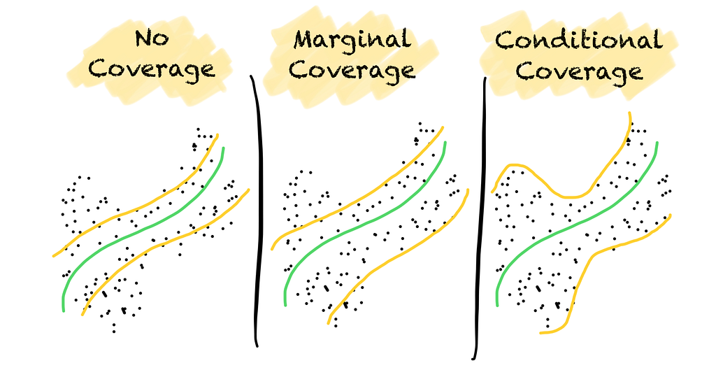
No coverage, marginal coverage, and conditional coverage for classification (left) and regression (right) problems. (Image by the author).
No coverage means that coverage is not guaranteed. The prediction region does not hold the true label with a predefined probability.
Marginal coverage means that coverage is guaranteed over all data points on average. The prediction region contains the true label at least with the stated probability. As coverage is only guaranteed over all data points, more errors may occur in one part of the space than in another. For example, the coverage might be small for minority classes in an imbalanced classification problem.
Conditional coverage means that coverage is guaranteed over all classes or data points. Errors occur in a balanced way. Conditional coverage, however, can only be approximated but not guaranteed.
Now we know why we need uncertainty quantification for ML and how helpful prediction regions look like.
But how can we quantify the uncertainty of a ML model?
Let’s assume we work for a company that classifies pictures of animals to understand how often a certain species appears in a given region. In the past, a person looked at each picture to identify the animal. This process took a long time. Hence, we build a model that classifies the animal in each picture. To be helpful, the model must be right in at least 90 % of the cases.
But the task is tricky. Our multiclass classification model only reaches an accuracy of 85% on our test set.
Hence, we want the model to tell us how certain it is about a picture. If the model is certain that its prediction is correct with a probability of more than 90 %, we use the model’s predicted class. Otherwise, we will have a human look at the picture.
But how can we tell if the model is certain or not? Let’s start with a naïve approach first.
Many classification models output the probability score of each class. Let’s take these and trust them. Every time, the model classifies a picture with a probability larger than 0.9 we trust the model. If the probability is lower, we give the picture to a human.
We give the model a picture of a dog. The model thinks this is a dog with a probability of 0.95. The model seems to be very certain. So, we trust the model.
For a picture of a cat the model, however, thinks the picture shows a giraffe with a probability of 0.8. Since the model’s probability is below our target of 90% probability, we discard the picture and give it to a human.
We do this with many pictures the model has not seen before.
Finally, we test the coverage of this approach for all pictures we classified. Unfortunately, we must realize that we have a smaller coverage than our aim of 90%. There are too many wrong predictions.
What did we do wrong?
Well, we trusted the probability score of the model.
But the score is not calibrated and does not guarantee the correct coverage for new data. The score would be calibrated if all classifications with a score of 0.9 would contain the true class 90% of the time. But this is not the case for the “probability” score of classification models.
Many approaches have the same problem, e.g., Platt scaling, isotonic regression, Bayesian predictive intervals, or bootstrapping. These are either not calibrated or rely on strong distribution assumptions.
But how can we achieve guaranteed coverage?
It seems like we only need to choose a better threshold.
Hence, we keep using the model’s “probability” score. But this time we change the score into a measure of uncertainty. In this case, one minus the model’s “probability” score for a class, i.e., 1 — s(x). The smaller the value, the more certain the model is about its prediction being the true class.
To determine the threshold, we use data the model has not seen during training. We calculate the non-conformity score of the true class for each sample in the set. Then we sort these scores from low (the model being certain) to high (the model being uncertain).
Sorting non-conformity scores of the true class for all samples in the calibration set (Image by the author).
Note that in this stage we only calculate the non-conformity score for the true class. We do not care about wether the model was rigth or wrong.
We use the resulting distribution to compute the threshold q_hat where 90% of the scores are lower. Our 90th percentile of the distribution. A score below this threshold will cover the true class with a probability of 90 %.
The threshold is determined by the 0.9 quantile of the distribution of non-conformity scores (Image by the author).
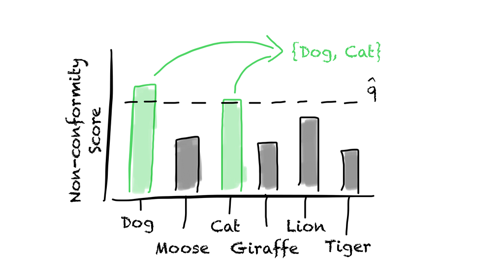
Now, every time we make a new prediction, we calculate the non-conformity score for all classes. Then we put all classes with a score lower than the threshold into our prediction set. That’s it.
With this, we can guarantee that the true class will be in the prediction set with a probability of 90 %.
All classes that have a non-conformity score above the threshold are put into the prediction set (Image by the author).
For our animal classification, we trust all predictions that only contain one animal in the prediction set. If the prediction set contains more than one class, we let a person check our classification.
Turning the theory into code
Not only is the approach easy to understand. The approach is also straightforward to implement. It only takes us three lines of code. It is that simple.
We follow the same steps, we did above.
We calculate the probability score for every sample in a calibration set that the model has not seen during training.
We determine the probability score of the true class for every sample.
We derive the threshold q_hat of our non-conformity score 1-s(x) based on the 0.9 quantile.
The only thing we have to account for is that we have a finite calibration set. Thus, we need to apply finite sample correction and multiply the 0.9 with (n+1)/n, in which n is the number of samples we use to calibrate out model.
Now, every time we run the model on unseen data, we can quantify the uncertainty of our model. This knowledge helps us in assessing the risk we are taking when making decisions based on our model.
In this article, I have shown you why you should care about quantifying your model’s uncertainty. I have also shown you how easy it is. However, I have only touched on the surface of uncertainty quantification. There is much more to learn.
Thus, I will dive deeper into uncertainty quantification in future articles. In the meantime, please feel free to leave some comments. Otherwise, see you in my next article.
We use cookies on our website to give you the most relevant experience by remembering your preferences and repeat visits. By clicking “Accept”, you consent to the use of ALL the cookies.
This website uses cookies to improve your experience while you navigate through the website. Out of these, the cookies that are categorized as necessary are stored on your browser as they are essential for the working of basic functionalities of the website. We also use third-party cookies that help us analyze and understand how you use this website. These cookies will be stored in your browser only with your consent. You also have the option to opt-out of these cookies. But opting out of some of these cookies may affect your browsing experience.
Necessary cookies are absolutely essential for the website to function properly. These cookies ensure basic functionalities and security features of the website, anonymously.
Cookie
Duration
Description
cookielawinfo-checkbox-analytics
11 months
This cookie is set by GDPR Cookie Consent plugin. The cookie is used to store the user consent for the cookies in the category "Analytics".
cookielawinfo-checkbox-functional
11 months
The cookie is set by GDPR cookie consent to record the user consent for the cookies in the category "Functional".
cookielawinfo-checkbox-necessary
11 months
This cookie is set by GDPR Cookie Consent plugin. The cookies is used to store the user consent for the cookies in the category "Necessary".
cookielawinfo-checkbox-others
11 months
This cookie is set by GDPR Cookie Consent plugin. The cookie is used to store the user consent for the cookies in the category "Other.
cookielawinfo-checkbox-performance
11 months
This cookie is set by GDPR Cookie Consent plugin. The cookie is used to store the user consent for the cookies in the category "Performance".
viewed_cookie_policy
11 months
The cookie is set by the GDPR Cookie Consent plugin and is used to store whether or not user has consented to the use of cookies. It does not store any personal data.
Functional cookies help to perform certain functionalities like sharing the content of the website on social media platforms, collect feedbacks, and other third-party features.
Performance cookies are used to understand and analyze the key performance indexes of the website which helps in delivering a better user experience for the visitors.
Analytical cookies are used to understand how visitors interact with the website. These cookies help provide information on metrics the number of visitors, bounce rate, traffic source, etc.
Advertisement cookies are used to provide visitors with relevant ads and marketing campaigns. These cookies track visitors across websites and collect information to provide customized ads.


