Tag: AI

  • Capture and Unlock Knowledge: A guide to foster your AI Business Plan

    Raul Vizcarra Chirinos

    Photo by Pawel Czerwinski on Unsplash

    AI solutions aren’t just a tool approach; it’s about well-understood use cases and ways to measure their impact

    The world we are shaping around AI includes different types of organizations: those building sophisticated AI technologies, others developing AI-based solutions, and finally, organizations that aim to use AI for positive impact or to support their businesses. When initiatives to deploy AI in the last group take place, capacity building and training are mostly oriented towards technical infrastructure, data ecosystems or technical skills; and although its significance is indisputable, we fail to understand that in most cases, AI solutions aren’t just a tool approach; it’s about well-understood use cases and ways to measure their impact. This guide aims to be useful to anyone leading AI initiatives and to complement any strategy aimed to enhance innovation capabilities through AI.

    “AI is not about its capabilities and promises, but also about how its used…” (The age of AI: And our Human Future -Kissinger, Schmidt, Huttenlocher)

    Every process of innovation through artificial intelligence consists of two parts: capturing knowledge and utilizing knowledge. This guide aims to demonstrate the strong relationship between both and the five dimensions that compose them (Use Cases, Early Wins, People, Technology, and Governance). Although they can independently coexist, together, they can significantly improve the chances of identifying and deploying AI-based solutions to make a substantial impact.

    I would like to clarify the intended scope of this guide. There is a lot of good work on this topic by consulting firms (Deloitte, McKinsey, BCG, Gartner, to name a few) and companies in the private sector or independent research ( Catalyst Fund,Profit.co,Dorien Herremans , to name a few). Therefore, it’s not my intention to present another bespoke conceptual framework or reinvent the wheel. In fact, some of the steps presented may sound very familiar to anyone leading an AI practice in a B2B tech consulting company. My intention is to move away from the abstraction of a conceptual framework and attempt to operationalize a set of steps with some tools that can help companies significantly improve their chances of identifying and deploying AI-based solutions to make a substantial impact.

    01: It’s all about Use Cases

    It’s not an AI tool approach; it’s all about USE CASES. This means that to increase our success rate on our AI project, we must identify real problems that affect our end users or the company we are working with. This really isn’t anything new, as most frameworks around AI strategy emphasize the importance of identifying good business cases as a starting point.

    This part is what I call “capturing knowledge”, and although everyone recognizes it as an important step, there is little information about the “How?” to do it. For this guide, I divide this capturing knowledge step into two dimensions: The identifying process and the prioritization process, which specifies parameters to help select which use case could be more relevant to engage with, and achieve Early Wins.

    Figure 01 Source: Author’s own creation

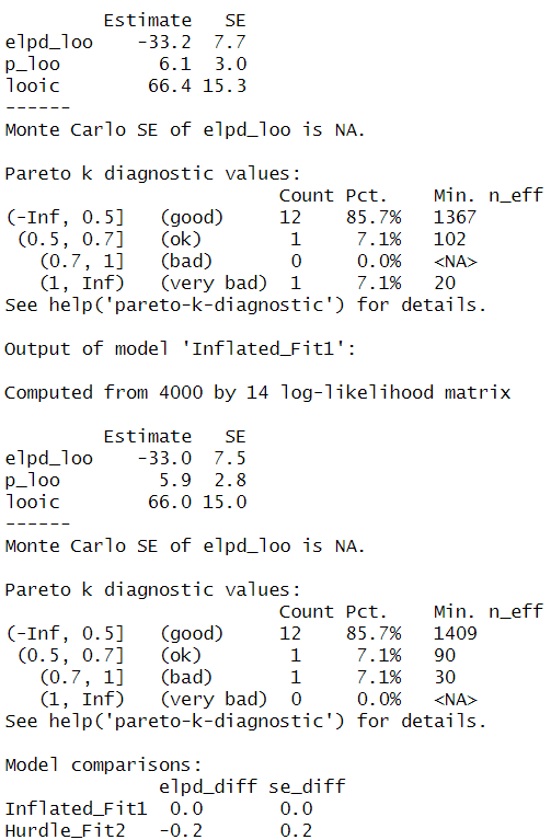
    How to identify good opportunities to deploy AI?

    01) Initiatives: What challenges does the industry you are in face?
    02) Use Cases: How is the company attempting to solve such challenges?
    03) Stakeholders: Which division/business unit does the challenge belong to? Who decides? Sponsors? Detractors?
    04) Insights: With what insights in the company are the challenges identified? Where do they come from?
    05) Data: What data do you have available to solve the challenge? Is it validated? Do you need more data?
    06) Tools: What tools (technology) does the company use to solve the challenge?

    02: Early Wins & Gains

    Every development follows an adoption curve; technology moves faster than the capacity of human beings to adopt it, and much faster than companies’ adaptation to this new customer behavior. This is kind of the essence of the “Collingridge Dilemma”, but it’s also relevant for understanding success in AI initiatives.

    Trajectories differ among companies; large corporations may have more tolerance for research, testing, and failure at the beginning in order to achieve significant results or radical innovations around AI. However, as mentioned before, many organizations are willing to use AI to support their businesses but face different dynamics, such as limited budgets and less tolerance for waiting for results. But Early wins aren’t just about profit or quick success, extracting some concepts from Kotter’s Change Management Framework, it’s about building momentum that excites people to pursue a common vision, to do things they’ve never done before, and to inspire discovery.

    Figure 02 Source: Author’s own creation

    Early wins and gains can be viewed from two different perspectives. From a business goal perspective, basic ideas have stayed the same in companies over time, any project that generates increased sales or reduces costs is always a good fit. Therefore, any AI initiative that demonstrates (meaning evidence with measurable data) the ability to drive efficiency, enable automation, or make predictions to accelerate decision-making processes would be a good place to start. From a Use Case perspective, it’s important to consider that NOT everything needs to be solved with AI, projects that can’t be addressed through traditional means, are data-rich, or involve large amounts of labor are likely to be well received. Finally, don’t forget that early executive buy-in is important; a strong endorsement can be the difference between reaching the deployment stage or getting stuck in the middle of the journey.

    “Wins are the molecules of results. They must be recognized, collected, and communicated — early and often — to track progress and energize volunteers to persist”. (The 8 Steps for Leading Change-John Kotter)

    03: A Team Committed to Continuous Learning

    Although it may sound like a cliché, people and skills are important, and almost every framework emphasizes it. However, while the size and expertise of the team will depend on the size of the company or budget, the velocity at which the team identifies potential AI initiatives to pursue and deploy them will exclusively depend on what I call “Continuous Learning”, inspired by the continuity concept behind practices like DevOps or MLOps and Peter Senge’s “The Learning Organization”. Let’s deconstruct the concept:

    Figure 03 Source: Author’s own creation

    The Skills You Have Vs. the Skills You Need: The artificial intelligence field encompasses a diverse range of skills and roles. As you begin to identify good AI initiatives, you may find situations where your team lacks the necessary skills to execute them. In the early stages of developing an AI Business Plan, focus on leveraging the skills that enable you to design, validate, and deploy “Early Wins”. Then, as these Early Wins are deployed, credibility is gained, and AI initiatives become more challenging, transition to acquire or develop more sophisticated skills.

    Awareness and Rituals: AI initiatives are neither a one-shot game nor a one-man show. It’s about continuously feeding the team with ideas to evaluate and pursue; some will succeed, and some may fail, but you need a pipeline of ideas continuously flowing. Primarily, you should have AI Initiatives flowing through three types of stages: Planting (stage of research, where the company’s Pains/Gains that could be resolved with AI are discussed), Growth (initiatives approved to proceed to a design, testing, or validation process), and Harvest (initiatives deployed and ready to scale or be replicated).

    To establish a funnel of AI initiatives continuously flowing through each stage, include in your AI business plan an assessment to identify:

    01) How does the team capture AI initiatives?
    02) How do the teams collaborate with other teams in the company, customers or end users to identify AI initiatives?
    03) How are relevant initiatives prioritized? Who determines their relevance?
    04) How are new AI initiatives tested or validated? How is the acquired knowledge documented and shared?

    Figure 04 Source: Author’s own creation

    The message is, Get out of the building! Organize daily meetings within the team and workshops with other business units, schedule visits with your customers and end users (not to sell them, but to understand their business pains) and conduct workshops with them as well.

    Remember that a funnel of AI initiatives is like a muscle; a continuous learning culture isn’t built in just one day. With that said, practices shouldn’t be done just once, but frequently, in order to transform awareness and rituals into attitudes and beliefs. In the long run, attitudes and beliefs are the ones that inspire discovery and push you to develop new capabilities and explore new grounds where you haven’t yet applied AI. One thing is for sure, if you don’t train the muscle frequently, ideas will stop flowing.

    04: Technology

    In technology, budget will be a limitation but not a restriction. Fortunately, we are living in exciting times in AI development, so for computing, modeling, testing, and deployment, you could benefit from either the open-source ecosystem built around AI or the free tiers offered by some service providers (Google, AWS, Azure, IBM cloud, Oracle cloud). While these come with restrictions, they can help with the research, design, and testing stages, which we aim to accelerate to validate good use cases for deployment.

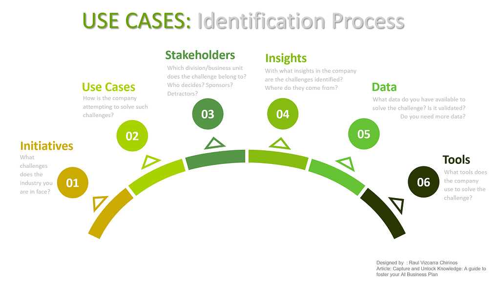
    So, what we aim to achieve is convenience; either building something from scratch to have full control over the architecture or leveraging pre-developed use cases and consuming them as a service, either entirely or as part of a mixed architecture. Inspired by the multi-step strategy playbook for managing digital disruption developed by the IMD-Digital Business Transformation Center, the following dimensions could help you choose the best technology to start with and how to scale:

    Figure 05 Source: Author’s own creation

    If you lead a small AI business unit or building one that needs to achieve “Erly Wins” quickly, perhaps your best option would be to leverage the open-source ecosystem, pre-built models, or prebuilt solutions. Rather than aiming for radical disruption with AI, aim for incremental benefits by using what has already been proven and tested. This approach is faster for validating ideas and designing, testing, and deploying AI initiatives, which is essential in the early stages to build confidence among your stakeholders for pursuing later disruptive challenges.

    Figure 06 Source: Author’s own creation

    If there is some flexibility in waiting for early successes (Early Wins), your best bet could be to start from scratch rather than using pre-existing solutions. While this approach can offer significant rewards in the long term, it also presents challenges in terms of managing feasibility, time constraints, and value. Results can wait, but they must be visible when the time comes.

    Figure 07 Source: Author’s own creation

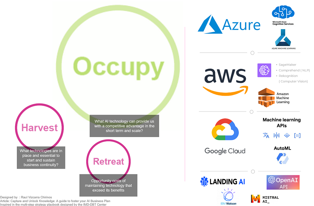
    Keep in mind that you can also achieve “Early Wins” when building AI initiatives from scratch (It’s all about use cases). For example, Python has lots of resources for developing supervised machine learning models, such as forecasting time series or predicting the probability of events like customer purchases, bill payments, or churn models for customer retention (Take into account that implementing these models will require your team to be stronger in statistical inference and modeling rather than technology). If your AI initiative involves unstructured data like text or videos, tools like PyTorch or the Hugging Face community offer open-source models for projects requiring text processing or video and image recognition. (If you’re interested, here are some examples: this one involves using Python for text processing and sentiment analysis, while this one utilizes Hugging Face resources for video analysis)

    Finally, while carrying out your technology assessment for your AI Business Plan, there are two considerations you must take into account:

    01) Balance between Skills and Technology: The technical skills that your team currently has, as well as those being developed, must align with the technology needed in the short term for Early Wins and the technology planned for future use. It goes both ways, if you intend to utilize a specific technology, ensure that your team has the appropriate skills to manage it or the ability to learn it quickly. Technical skills can be found in the labor market (depending on the technical skills required, they may come at a price) or developed internally, but requires time, and time is a constraint when pursuing Early Wins.

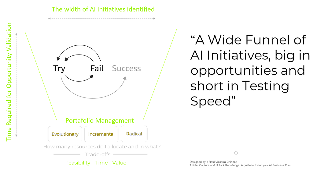
    02) Wide Funnel-Fast Testing: The balance between validated AI initiatives, People, and Technology should result in a broad funnel of AI initiatives, big in opportunities and efficient in testing speed. The portfolio should continuously include a mix of AI initiatives: Incremental AI initiatives for early wins and a steady stream of income, Evolutionary AI initiatives to replicate successful deployments in other markets, and Disruptive AI initiatives to remain at the forefront and anticipate future trends. The portfolio-mix depends on the tolerance for waiting for early wins. AI is not a solitary endeavor; it involves managing a portfolio of AI initiatives. The key is to continually expand the funnel and shorten the testing process so that AI initiatives can be tested and deployed quickly at low cost.(For further insights on managing an innovation portfolio, consider reading this article)

    Figure 08 Source: Author’s own creation

    05: Governance

    A famous quote states, “Normal is an illusion; what is normal for the spider is chaos for the fly”. Recent years have highlighted the reality that we live in uncertain and dynamic business environments, where resilience and the ability to adapt quickly are essential assets. Applied to AI initiatives, this means that in order to deploy and scale rapidly, we need Machine Learning pipelines that are efficient, support frequent execution, and are reliable. For data management, good work has been done with frameworks like DAMA-DMBOK and DataOps, and for AI, we have MLOps.

    Figure 09 Source: Author’s own creation

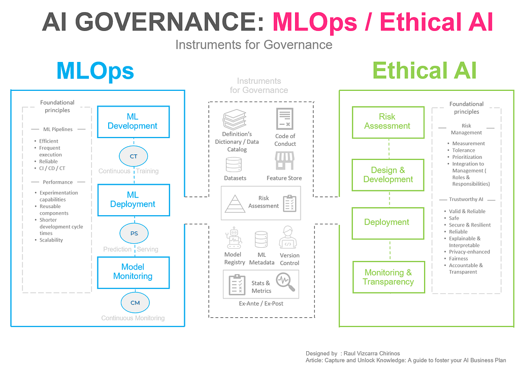
    MLOps: Deployment presents challenges such as potential issues with the handoff between Data Scientists and IT teams, tracking of the development stage, and impacts produced by changes in data or model drifting. With MLOps, we gain several benefits. First, in the Development stage, it’s all about “experimentation” (data exploration, feature engineering, model prototyping, and validation) while keeping records and knowledge of this process. Second, in version controlling, we answer questions like who?, why?, and how? for future compliance and reusable components (such as a feature store for data). Lastly, in monitoring for changes in data or model deviations and ensuring model fairness. You can find a useful guide in Google’s Practitioners Guide to MLOps.

    Ethical AI Governance: Another issue related to AI governance is compliance. While the debate on regulatory frameworks is ongoing (with some in the final stages of implementation), companies can begin with self-regulated frameworks for risk assessment, controlled testing environments, development protocols, and ongoing monitoring to achieve ethical and responsible AI deployments. In this article, I share some ideas of a self-regulated framework based on the EU AI Act that could be useful for your AI business plan. Another valuable resource that is essential to read for guidance is the Artificial Intelligence Risk Management Framework from the US National Institute of Standards and Technology (NIST).

    FINAL THOUGHT

    The idea of human-like machines has always fascinated humanity, as described in a 2022 essay by Erik Brynjolfsson from Stanford University, where he also discusses its economic impacts, emphasizing the benefits of augmenting human capabilities over mere automation. Both automation and augmentation foster productivity; the difference is that the latter pushes humankind to do things they never could before, inspiring discovery and boosting living standards.

    It’s certain that we will continue to search for technology that replicates human behavior. The difference lies in how we perceive concepts like automation and AI. Focusing only on mimicking the world as it is, overlooks all the new things that we can make with AI to shape a better tomorrow.

    Thank you for reading!, Did I miss anything? Your suggestions are always welcome and keep the conversation going.


    Capture and Unlock Knowledge: A guide to foster your AI Business Plan was originally published in Towards Data Science on Medium, where people are continuing the conversation by highlighting and responding to this story.

    Originally appeared here:
    Capture and Unlock Knowledge: A guide to foster your AI Business Plan

    Go Here to Read this Fast! Capture and Unlock Knowledge: A guide to foster your AI Business Plan

  • Feature Engineering that Makes Business Sense

    Feature Engineering that Makes Business Sense

    Guillaume Colley

    The author outlines three ways to expand your machine learning feature set with features that represent explainable behaviors and that…

    Originally appeared here:
    Feature Engineering that Makes Business Sense

    Go Here to Read this Fast! Feature Engineering that Makes Business Sense

  • Public Transport Accessibility in Python

    Public Transport Accessibility in Python

    Milan Janosov

    In this piece, I explore the availability of public transport by using GTFS data and Python-based spatial analytics libraries.

    Originally appeared here:
    Public Transport Accessibility in Python

    Go Here to Read this Fast! Public Transport Accessibility in Python

  • Improving the Analysis of Object (or Cell) Counts with Lots of Zeros

    Improving the Analysis of Object (or Cell) Counts with Lots of Zeros

    Daniel Manrique-Castano

    An approach using hurdle and zero-inflated models with brms

    NeuN and GFAP staining in a mouse brain following cerebral ischemia. Manrique-Castano et al. (2024) (CC-BY).

    Counting is a fundamental task in biomedical research, particularly when analyzing cell populations. Imagine staring at countless cells within a tiny brain region — sometimes numbering in the hundreds or thousands. Yet, in other areas, these numbers may dwindle to few or even none.

    The challenge arises in how we analyze these counts. For large numbers, linear models, which assume a normal distribution, often serve as a reasonable approximation. Though not optimal, they provide a logical framework for initial analysis. However, the scenario shifts dramatically when cell counts are low or predominantly zeros. Here, traditional linear models (like those t-tests we run in GraphPad) falter, losing their effectiveness and relevance.

    As researchers, we must strive for better, going beyond t-tests and ANOVAs. This post aims to explore alternative statistical methods that more accurately reflect the realities of our data, especially when dealing with low or zero counts. By embracing more fitted approaches, we can enhance the precision of our findings and deepen our understanding of our cell populations.

    First, let’s load the necessary libraries and create a visual theme for our plots.

    library(ggplot2)
    library(brms)
    library(ggdist)
    library(easystats)
    library(dplyr)
    library(modelr)
    library(patchwork)
    library(tibble)
    library(tidybayes)

    logit2prob <- function(logit){
    odds <- exp(logit)
    prob <- odds / (1 + odds)
    return(prob)
    }

    Plot_theme <- theme_classic() +
    theme(
    plot.title = element_text(size=18, hjust = 0.5, face="bold"),
    plot.subtitle = element_text(size = 10, color = "black"),
    plot.caption = element_text(size = 12, color = "black"),
    axis.line = element_line(colour = "black", size = 1.5, linetype = "solid"),
    axis.ticks.length=unit(7,"pt"),

    axis.title.x = element_text(colour = "black", size = 16),
    axis.text.x = element_text(colour = "black", size = 16, angle = 0, hjust = 0.5),
    axis.ticks.x = element_line(colour = "black", size = 1),

    axis.title.y = element_text(colour = "black", size = 16),
    axis.text.y = element_text(colour = "black", size = 16),
    axis.ticks.y = element_line(colour = "black", size = 1),

    legend.position="right",
    legend.direction="vertical",
    legend.title = element_text(colour="black", face="bold", size=12),
    legend.text = element_text(colour="black", size=10),

    plot.margin = margin(t = 10, # Top margin
    r = 2, # Right margin
    b = 10, # Bottom margin
    l = 10) # Left margin
    )

    What is the issue with counting zeros?

    In many studies, like the one shown in the graph by (1), we encounter the challenge of low cell counts, particularly where one group — marked here in black — appears to be dominated by zero counts. This scenario is not uncommon in biomedical literature, where straightforward linear models are frequently applied to analyze such data.

    Figure 1: CD3+ cells by Baraibar et. al (2020) (CC-BY)

    However, the use of these models in cases of low or zero counts can be problematic. Without access to the original datasets — which researchers often do not share — it’s difficult to evaluate the efficacy of the analysis fully. To better understand this issue, let’s consider a separate dataset from my own research. Several years ago, I undertook the task of counting BrdU+ cells following an ischemic event in a specific brain area called the subventricular zone (SVZ). This particular experience inclined me to evaluate more suitable statistical approaches.

    These are the data:

    Svz_data <- read.csv("Data/CellCounts.csv")
    Svz_data$Hemisphere <- factor(Svz_data$Hemisphere, levels = c("Contralateral", "Ipsilateral"))
    head(Svz_data)

    We can visualize that the contralateral hemisphere has a lot of null cell counts. We can have a better angle if we use a boxplot:

    ggplot(Svz_data, aes(x = Hemisphere, y = Cells)) +
    geom_boxplot() +
    labs(x = "Hemisphere", y = "Number of cells", title = "Cells by hemisphere") +
    Plot_theme +
    theme(legend.position = "top", legend.direction = "horizontal")
    Figure 2: Cell counts by hemisphere

    Figure 2 vividly illustrates the substantial disparities in cell counts across hemispheres. To examine what happens when we apply a typical (and horrific) linear model to such data, we’ll proceed with a practical demonstration using the brms. This will help us understand the effects of these variations when analyzed under a traditional framework predicated on normal distribution assumptions.

    In this example, I’ll fit a linear model where the factor variable “hemisphere” is the sole predictor of the cell counts:

    lm_Fit <- brm(Cells ~ Hemisphere, 
    data = Svz_data,
    # seed for reproducibility purposes
    seed = 8807,
    control = list(adapt_delta = 0.99),
    # this is to save the model in my laptop
    file = "Models/2024-04-19_CountsZeroInflated/lm_Fit.rds",
    file_refit = "never")

    # Add loo for model comparison
    lm_Fit <-
    add_criterion(lm_Fit, c("loo", "waic", "bayes_R2"))

    Are you willing to bet on what the results will be? Let’s find out:

    If you like, you can fit a frequentist (OLS) model with lm and you will certainly get the same results. In these results, the intercept represents an estimate of cell counts for the contralateral hemisphere, which serves as our reference group. However, a significant inconsistency arises when employing a normal distribution for data that includes numerous zero counts or values close to zero. In such cases, the model is inappropriately “forced” to predict that cell counts in our hemisphere could be negative, such as -1 to -2 cells, with a confidence interval ranging from -1.5 to 3.7. This prediction is fundamentally flawed because it disregards the intrinsic nature of cells as entities that can only assume non-negative integer values.

    This issue stems from the fact that our model, in its current form, does not comprehend the true characteristics of the data it’s handling. Instead, it merely follows our directives — albeit incorrectly — to fit the data to a linear model. This common oversight often leads researchers to further exacerbate the problem by applying t-tests and ANOVAs, thereby superimposing additional analysis onto a model that is fundamentally unsound. It is imperative that we, as researchers, recognize and harness our capabilities and tools to develop and utilize more appropriate and logically sound modeling methods that respect the inherent properties of our data.

    Let’s plot the results using the great TidyBayes package (2) by the great Matthew Kay

    Svz_data %>%
    data_grid(Hemisphere) %>%
    add_epred_draws(lm_Fit) %>%
    ggplot(aes(x = .epred, y = Hemisphere)) +
    labs(x = "Number of cells") +
    stat_halfeye() +
    geom_vline(xintercept = 0) +
    Plot_theme
    Figure 3: Posterior distribution for cell counts by hemisphere

    We can also see this inconsistency if we perform pp_check to compare the observations with the model predictions:

    Figure 4: Posterior predictive checks gaussian model

    Once again, we encounter irrational predictions of cell counts falling below zero. As scientists, it’s crucial to reflect on the suitability of our models in relation to the data they are intended to explain. This consideration guides us toward generative models, which are build under the premise that they could plausibly have generated the observed data. Clearly, the linear model currently in use falls short of this criterion. It predicts impossible negative values for cell counts. Let’s try to find out a better model.

    Working with lots of zeros

    A zero-inflated model effectively captures the nuances of datasets characterized by a preponderance of zeros. It operates by distinguishing between two distinct processes: 1) Determining whether the result is zero, and 2) predicting the values for non-zero results. This dual approach is particularly apt for asking questions like, “Are there any cells present, and if so, how many?”

    For handling datasets with an abundance of zeros, we employ models such as hurdle_poisson() and Zero_inflated_poisson, both designed for scenarios where standard count models like the Poisson or negative binomial models prove inadequate (3).Loosely speaking, a key difference between hurdle_poisson() and Zero_inflated_poisson is that the latter incorporates an additional probability component specifically for zeros, enhancing their ability to handle datasets where zeros are not merely common but significant. We’ll see the impact these features have in our modeling strategy using brms.

    Fitting a hurdle_poisson model

    Let’s start by using the hurdle_poisson() distribution in our modeling scheme:

    Hurdle_Fit1 <- brm(Cells ~ Hemisphere, 
    data = Svz_data,
    family = hurdle_poisson(),
    # seed for reproducibility purposes
    seed = 8807,
    control = list(adapt_delta = 0.99),
    # this is to save the model in my laptop
    file = "Models/2024-04-19_CountsZeroInflated/Hurdle_Fit1.rds",
    file_refit = "never")

    # Add loo for model comparison
    Hurdle_Fit1 <-
    add_criterion(Hurdle_Fit1, c("loo", "waic", "bayes_R2"))

    Let’s see the results using the standard summary function.

    summary(Hurdle_Fit1)

    Given this family distribution, the estimates are shown in the log scale (mu = log). In practical terms, this means that the number of cells in the contralateral subventricular zone (SVZ) can be expressed as exp(1.11) = 3.03. Similarly, the ipsilateral hemisphere is estimated to have exp(1.07) = 2.91 times the number of cells. These results align well with our expectations and offer a coherent interpretation of the cell distribution between the two hemispheres.

    Additionally, the hu parameter within the “Family Specific Parameters” sheds light on the likelihood of observing zero cell counts. It indicates a 38% probability of zero occurrences. This probability highlights the need for a zero-inflated model approach and justifies its use in our analysis.

    To better visualize the implications of these findings, we can leverage the conditional_effects function. This tool in the brms package allows us to plot the estimated effects of different predictors on the response variable, providing a clear graphical representation of how the predictors influence the expected cell counts.

    Hurdle_CE <- 
    conditional_effects(Hurdle_Fit1)

    Hurdle_CE <- plot(Hurdle_CE,
    plot = FALSE)[[1]]

    Hurdle_Com <- Hurdle_CE +
    Plot_theme +
    theme(legend.position = "bottom", legend.direction = "horizontal")


    Hurdle_CE_hu <-
    conditional_effects(Hurdle_Fit1, dpar = "hu")

    Hurdle_CE_hu <- plot(Hurdle_CE_hu,
    plot = FALSE)[[1]]

    Hurdle_hu <- Hurdle_CE_hu +
    Plot_theme +
    theme(legend.position = "bottom", legend.direction = "horizontal")

    Hurdle_Com | Hurdle_hu
    Figure 5: Conditional effects for the hurdle fit

    These plots draw a more logical picture than our first model. The graph on the left shows the two parts of the model (“mu” and “hu”). Also, if this model is suitable, we should see more aligned predictions when using pp_check:

    pp_check(Hurdle_Fit1, ndraws = 100) +
    labs(title = "Hurdle regression") +
    theme_classic()
    Figure 6: Posterior predictive checks hurdle model

    As expected, our model predictions have a lower boundary at 0.

    Modeling the dispersion of the data

    Observing the data presented in the right graph of Figure 5 reveals a discrepancy between our empirical findings and our theoretical understanding of the subject. Based on established knowledge, we expect a higher probability of non-zero cell counts in the subventricular zone (SVZ) of the ipsilateral hemisphere, especially following an injury. This is because the ipsilateral SVZ typically becomes a hub of cellular activity, with significant cell proliferation post-injury. Our data, indicating prevalent non-zero counts in this region, supports this biological expectation.

    However, the current model predictions do not fully align with these insights. This divergence underscores the importance of incorporating scientific understanding into our statistical modeling. Relying solely on standard tests without contextual adaptation can lead to misleading conclusions.

    To address this, we can refine our model by specifically adjusting the hu parameter, which represents the probability of zero occurrences. This allows us to more accurately reflect the expected biological activity in the ipsilateral hemisphere’s SVZ. We build then a second hurdle model:

    Hurdle_Mdl2 <- bf(Cells ~ Hemisphere, 
    hu ~ Hemisphere)

    Hurdle_Fit2 <- brm(
    formula = Hurdle_Mdl2,
    data = Svz_data,
    family = hurdle_poisson(),
    # seed for reproducibility purposes
    seed = 8807,
    control = list(adapt_delta = 0.99),
    # this is to save the model in my laptop
    file = "Models/2024-04-19_CountsZeroInflated/Hurdle_Fit2.rds",
    file_refit = "never")

    # Add loo for model comparison
    Hurdle_Fit2 <-
    add_criterion(Hurdle_Fit2, c("loo", "waic", "bayes_R2"))

    Let’s see first if the results graph aligns with our hypothesis:

    Hurdle_CE <- 
    conditional_effects(Hurdle_Fit2)

    Hurdle_CE <- plot(Hurdle_CE,
    plot = FALSE)[[1]]

    Hurdle_Com <- Hurdle_CE +
    Plot_theme +
    theme(legend.position = "bottom", legend.direction = "horizontal")


    Hurdle_CE_hu <-
    conditional_effects(Hurdle_Fit2, dpar = "hu")

    Hurdle_CE_hu <- plot(Hurdle_CE_hu,
    plot = FALSE)[[1]]

    Hurdle_hu <- Hurdle_CE_hu +
    Plot_theme +
    theme(legend.position = "bottom", legend.direction = "horizontal")

    Hurdle_Com | Hurdle_hu
    Figure 7: Conditional effects for the hurdle fit 2

    This revised modeling approach seems to be a substantial improvement. By specifically accounting for the higher probability of zero counts (~75%) in the contralateral hemisphere, the model now aligns more closely with both the observed data and our scientific knowledge. This adjustment not only reflects the expected lower cell activity in this region but also enhances the precision of our estimates. With these changes, the model now offers a more nuanced interpretation of cellular dynamics post-injury. Let’s see the summary and the TRANSFORMATION FOR THE hu parameters (do not look at the others) to visualize them in a probability scale using the logit2prob function we created at the beginning.

    logit2prob(fixef(Hurdle_Fit2))

    Although the estimates for the number of cells are similar, the hu parameters (in the logit scale) tells us that the probability for seeing zeros in the contralateral hemisphere is:

    Conversely:

    Depicts a drastic reduction to about 0.23% probability of observing zero cell counts in the injured (ipsilateral) hemisphere. This is a remarkable change in our estimates.

    Now, let’s explore if a zero_inflated_poisson() distribution family changes these insights.

    Fitting a zero-inflated Poisson model

    As we modeled the broad variations in cell counts between the ipsilateral and contralateral hemispheres using the hu parameter, we’ll fit as well these two parts of the model in our zero_inflated_poisson(). Here, the count part of the model uses a “log” link, and the excess of zeros is modeled with a “logit” link. These are linked functions associated to the distribution family that we’ll not discuss here.

    Inflated_mdl1 <- bf(Cells ~ Hemisphere,
    zi ~ Hemisphere)

    Inflated_Fit1 <- brm(
    formula = Inflated_mdl1,
    data = Svz_data,
    family = zero_inflated_poisson(),
    # seed for reproducibility purposes
    seed = 8807,
    control = list(adapt_delta = 0.99),
    # this is to save the model in my laptop
    file = "Models/2024-04-19_CountsZeroInflated/Inflated_Fit.rds",
    file_refit = "never")

    # Add loo for model comparison
    Inflated_Fit1 <-
    add_criterion(Inflated_Fit1, c("loo", "waic", "bayes_R2"))

    Before we look at the results, let’s do some basic diagnostics to compare the observations and the model predictions.

    set.seed(8807)

    pp_check(Inflated_Fit1, ndraws = 100) +
    labs(title = "Zero-inflated regression") +
    theme_classic()
    Figure 8: Model diagnostics for the zero-inflated regression

    From Figure 8, we can see that the predictions deviate from the observed data in a similar way to the hurdle model. So, we have no major changes up to this point.

    Let’s see the numerical results:

    logit2prob(fixef(Inflated_Fit1))

    Here, we do see tiny changes in the estimates. The estimate for the number of cells is similar with small changes in the credible intervals. Otherwise, the parameter for the number of zeros seems to experience a larger shift. Let’s see if this has any effect on our conclusions:

    Indicates that there is approximately a 77% probability of observing zero counts in the reference hemisphere. Now, for the injured hemisphere, we have:

    Again, this signals a drastic reduction in observing zero cell counts in the injured (ipsilateral) hemisphere. Evaluating the results using scientific knowledge, I would say that both models provide similarly sound predictions. The graphical results for our zero_inflated_poisson model are as follows:

    Inflated_CE <- 
    conditional_effects(Inflated_Fit1)

    Inflated_CE <- plot(Inflated_CE,
    plot = FALSE)[[1]]

    Inflated_Com <- Inflated_CE +
    Plot_theme +
    theme(legend.position = "bottom", legend.direction = "horizontal")


    Inflated_CE_zi <-
    conditional_effects(Inflated_Fit1, dpar = "zi")

    Inflated_CE_zi <- plot(Inflated_CE_zi,
    plot = FALSE)[[1]]

    Inflated_zi <- Inflated_CE_zi +
    Plot_theme +
    theme(legend.position = "bottom", legend.direction = "horizontal")

    Inflated_Com | Inflated_zi
    Figure 9: Conditional effects for the Inflated fit

    The results seem analogous to those of the hurdle model. However, we can observe that the estimates for the probability of 0 in the contralateral hemisphere is more restrictive for the zero_inflated_poisson. The reason is, as I explained at the beginning, that the zero-inflated model locates a larger probability of zeros than the hurdle_poisson distribution. Let’s compare the models to finish this post.

    Model comparison

    We carry out leave-one-out cross-validation using the the loo package (4, 5). WAIC (6) is another approach you can explore in this post.

    loo(Hurdle_Fit2, Inflated_Fit1)

    Even though if our model predictions are alike, the “pareto-k-diagnostic” indicates that the hurdle_poisson model has 1 very bad value, whereas this value shifts to bad in the zero_inflated_poisson(). I judge that this “bad and very bad” value may be a product of the extreme observation that we see as a black dot in the contralateral count in Figure 2. We could fit another model excluding this value and re-evaluate the results. However, this procedure would only aim to evaluate the effect of this extreme observation and inform the audience of a possible bias in the estimates (which should be fully reported). This is a thorough and transparent way to interpret the data. I wrote another post concerning extreme values that may be of interest to you.

    I conclude that the modeling performed in this post is a more appropriate approach than a naive linear model based on a Gaussian distribution. It is an ethical and professional responsibility of scientists to use the most appropriate statistical modeling tools available. Fortunately, brms exists!

    I would appreciate your comments or feedback letting me know if this journey was useful to you. If you want more quality content on data science and other topics, you might consider becoming a medium member.

    In the future, you can find an updated version of this post on my GitHub site.

    • All images, unless otherwise stated, were generated using the displayed R code.

    References

    1.I. Baraibar, M. Roman, M. Rodríguez-Remírez, I. López, A. Vilalta, E. Guruceaga, M. Ecay, M. Collantes, T. Lozano, D. Alignani, A. Puyalto, A. Oliver, S. Ortiz-Espinosa, H. Moreno, M. Torregrosa, C. Rolfo, C. Caglevic, D. García-Ros, M. Villalba-Esparza, C. De Andrea, S. Vicent, R. Pío, J. J. Lasarte, A. Calvo, D. Ajona, I. Gil-Bazo, Id1 and PD-1 Combined Blockade Impairs Tumor Growth and Survival of KRAS-mutant Lung Cancer by Stimulating PD-L1 Expression and Tumor Infiltrating CD8+ T Cells. Cancers. 12, 3169 (2020).

    2. M. Kay, tidybayes: Tidy data and geoms for Bayesian models (2023; http://mjskay.github.io/tidybayes/).

    3. C. X. Feng, A comparison of zero-inflated and hurdle models for modeling zero-inflated count data. Journal of Statistical Distributions and Applications. 8 (2021), doi:10.1186/s40488–021–00121–4.

    4. A. Vehtari, J. Gabry, M. Magnusson, Y. Yao, P.-C. Bürkner, T. Paananen, A. Gelman, Loo: Efficient leave-one-out cross-validation and WAIC for bayesian models (2022) (available at https://mc-stan.org/loo/).

    5. A. Vehtari, A. Gelman, J. Gabry, Practical Bayesian model evaluation using leave-one-out cross-validation and WAIC. Statistics and Computing. 27, 1413–1432 (2016).

    6. A. Gelman, J. Hwang, A. Vehtari, Understanding predictive information criteria for Bayesian models. Statistics and Computing. 24, 997–1016 (2013).


    Improving the Analysis of Object (or Cell) Counts with Lots of Zeros was originally published in Towards Data Science on Medium, where people are continuing the conversation by highlighting and responding to this story.

    Originally appeared here:
    Improving the Analysis of Object (or Cell) Counts with Lots of Zeros

    Go Here to Read this Fast! Improving the Analysis of Object (or Cell) Counts with Lots of Zeros

  • The Math Behind Recurrent Neural Networks

    Cristian Leo

    Dive into RNNs, the backbone of time series, understand their mathematics, implement them from scratch, and explore their applications

    Originally appeared here:
    The Math Behind Recurrent Neural Networks

    Go Here to Read this Fast! The Math Behind Recurrent Neural Networks