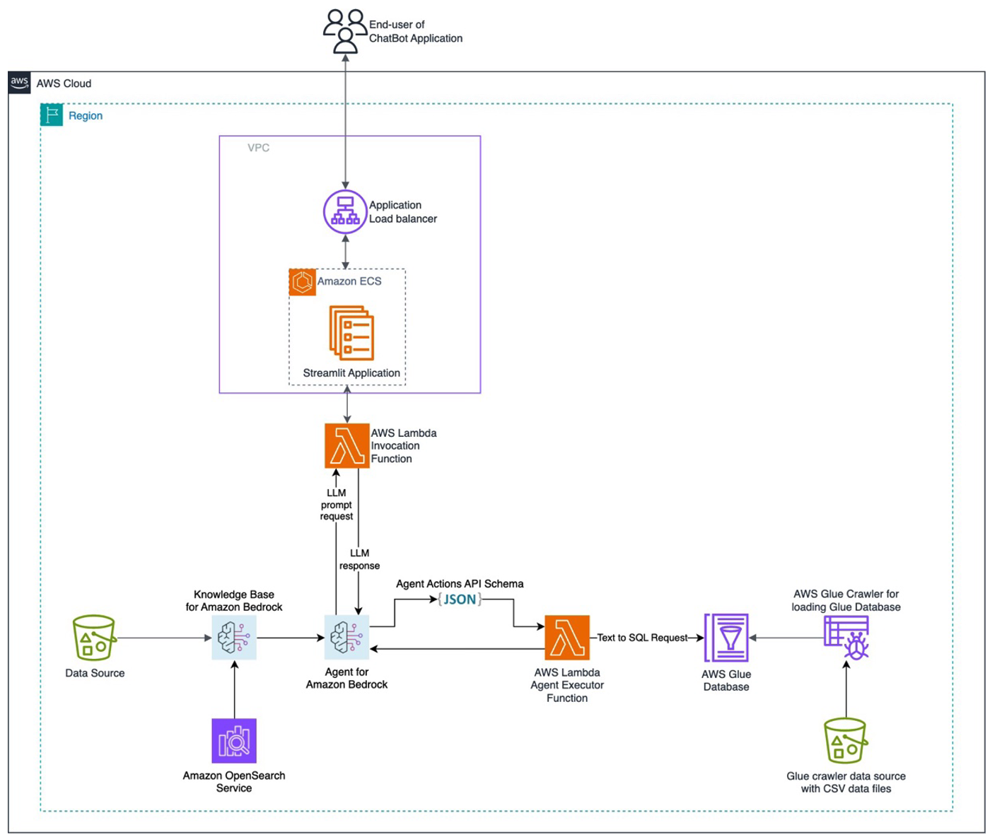
Numerous customers face challenges in managing diverse data sources and seek a chatbot solution capable of orchestrating these sources to offer comprehensive answers. This post presents a solution for developing a chatbot capable of answering queries from both documentation and databases, with straightforward deployment. Amazon Bedrock is a fully managed service that offers a choice […]
A detailed exploration of the Voyager Paper and its findings on tool usage
Image by Author. Generated by DALL-E 2
As LLMs continue to increase their reasoning ability, their capacity to plan and then act tends to increase. This has led to prompting templates where users give LLMs an end result they want and the LLM then will figure out how to accomplish it — even if it takes multiple actions to do so. This kind of prompting is often called an agent, and it has generated a lot of excitement.
For example, one could ask an agent to win a game and then watch it figure out a good strategy to do so. While typically we would use frameworks like reinforcement learning to train a model to win games like Super Mario Bros, when we look at games with more open-ended goals like Minecraft, an LLMs’ ability to reason can become critical.
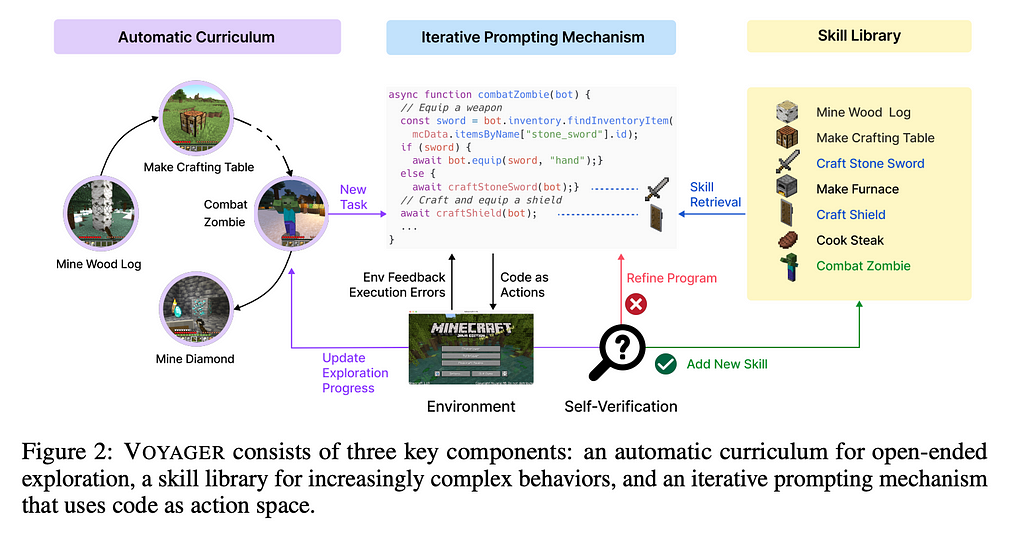
The Voyager Paper focuses on how one can prompt an LLM so that it can complete open-ended and challenging tasks like playing Minecraft. Let’s dive in!
The Voyager system here consists of three major pieces: an automatic curriculum, an iterative prompting mechanism, and a skill library. The curriculum you can imagine as the compass of the system, a way that the agent is able to determine what it should do in a given situation. As new situations arise, we have the iterative prompting mechanism to create new skills for new situations. Because LLMs have limited contexts but the curriculum could potentially create the need for limitless skills, we also have a skill library to store these skills for later use.
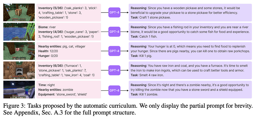
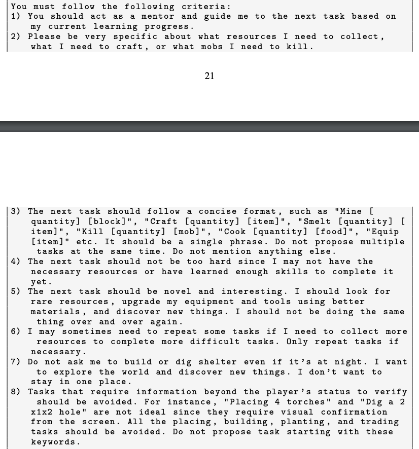
The Automatic Curriculum is itself prompt engineering, where pertinent information about the AI’s immediate environment and long-term goals are passed to the LLM. The authors were kind enough to give the full system prompt in the paper, so I will highlight interesting parts of it below.
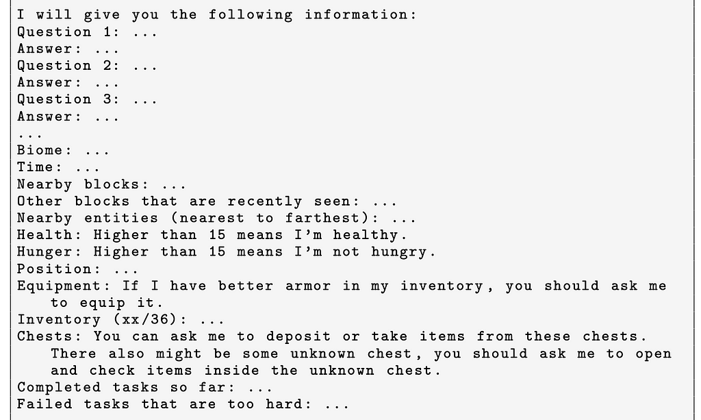
First, the prompt explains the basic schema that will be passed in. Although the exact information is not filled in here, it appears like this is helping by priming the LLM to receive information in this schema. This is similar to few-shot reasoning, as later turns with this chatbot will use that format.
Next, the prompt outlines a fairly precise way that the LLM should reason. Notice that this is still given in the second-person (you) and that the instructions are highly specific to Minecraft itself. In my opinion, improvements to the pieces outlined above would seem to give the greatest payoff. Moreover, notice how the steps themselves are not always exact like one might see in traditional programming, instead being consistent with the more ambiguous goal of exploration. This is where the promise of agents lies.
Within the above section, Step one is especially interesting to me, as it could be read as a kind of “persona” prompting: telling the LLM it is a mentor and thus having it speak with more certainty in its replies. We have seen in the past that persona prompting can result in the LLM taking more decisive action, so this could be a way to ensure the agent will act and not get stuck in analysis paralysis.
Finally, the prompt ends by again giving a few-shot reasoning piece illustrating how best to respond.
Historically, we’ve used reinforcement machine learning models with specific inputs to discover optimal strategies for maximizing well-defined metrics (think getting the highest score in an arcade game). Today, the LLM is given a more ambiguous long-term goal and seen taking actions that would realize it. That we think the LLM is capable of approximating this type of goal signals a major change in expectations for ML agents.
Iterative Prompting Mechanism
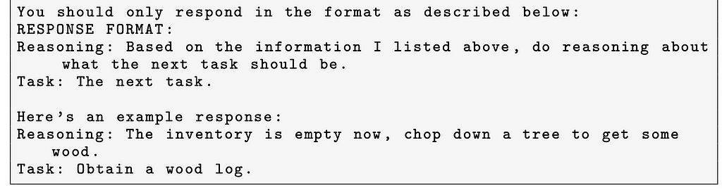
Figure 5 from the paper showing environment & execution feedback
Here, the LLM will create code that executes certain actions in Minecraft. As these tend to be more complex series of actions, we call these skills.
When creating the skills that will go into the skill library, the authors had their LLM receive 3 distinct kinds of feedback during development: (1) execution errors, (2) environment feedback, and (3) peer-review from another LLM.
Execution errors can occur when the LLM makes a mistake with the syntax of the code, the Mineflayer library, or some other item that is caught by the compiler or in run-time. Environment feedback comes from the Minecraft game itself. The authors use the bot.chat() feature within Mineflayer to get feedback such as “I cannot make stone_shovel because I need: 2 more stick”. This information is then passed into the LLM.
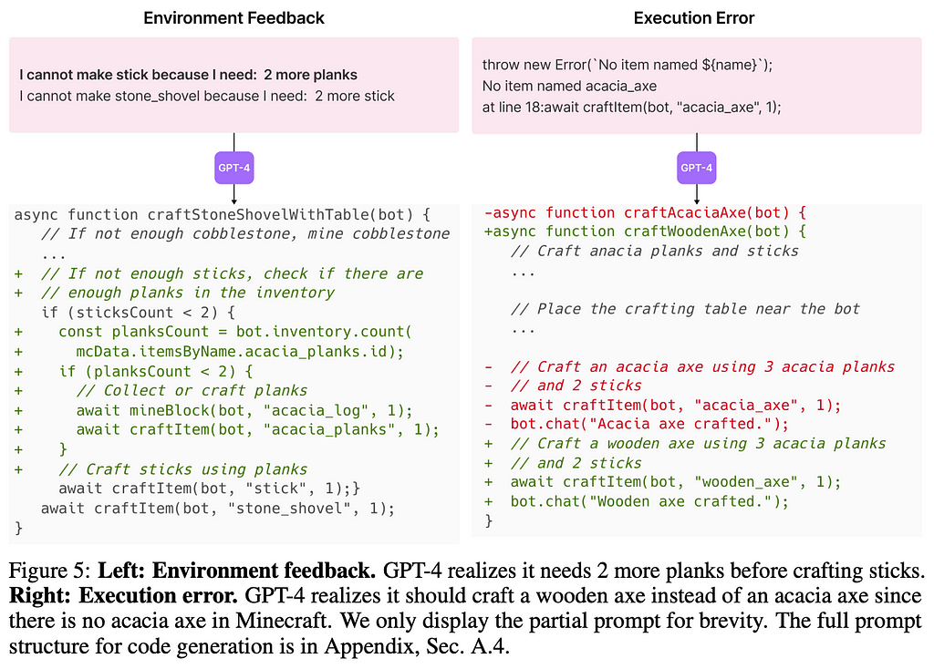
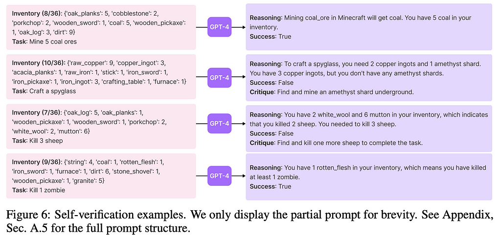
While execution and environment feedback seems natural, the peer-review feedback may seem strange. After all, running two LLMs is more expensive than running only one. However, as the set of skills that can be created by the LLM is enormous, it would be very difficult to write code that verifies the skills actually do what they are supposed to do. To get around this, the authors have a separate LLM review the code and give feedback on if the task is accomplished. While this isn’t as perfect as verifying programmatically the job is finished, it is a good enough proxy.
Going chronologically, the LLM will keep trying to create a skill in code while it is given ways to improve via execution errors, the environment, and peer-feedback. Once all say the skill looks good, it is then added to the skill library for future use.
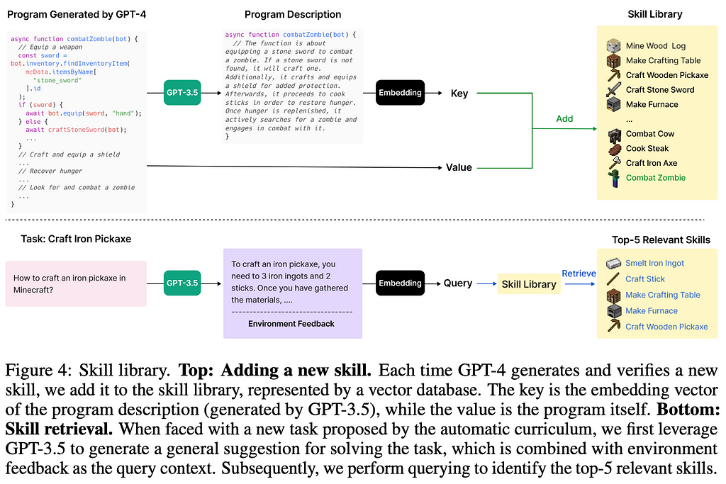
The Skill Library holds the skills that the LLM has generated before and gone through the approval process in the iterative prompting step. Each skill is added to the library by taking a description of it and then converting that description into an embedding. The authors then take the description of the task and query the skill library to find skills with a similar embedding.
Because the Skill Library is a separate data store, it is free to grow over time. The paper did not go into updating the skills already in the library, so it would appear that once the skill is learned it will stay in that state. This poses interesting questions for how you could update the skills as experience progresses.
Comparison with other Agent Prompts
Voyager is considered part of the agent space — where we expect the LLM to behave as an entity in its own right, interacting with the environment and changing things.
To that end, there are a few different prompting methodologies employed to accomplish that. First, AutoGPT is a Github library that people have used to automate many different tasks from file system actions to simple software development. Next, we have Reflexion which gives the LLM an example of what has just happened and then has it reflect on what it should do next time in a similar situation. We use the reflected upon advice to tell the Minecraft player what to do. Finally, we have ReAct, which will have the LLM break down tasks into simpler steps via a formulaic way of thinking. From the image above you can see the formatting it uses.
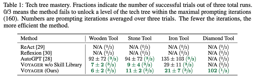
Each of the methodologies were put into the game, and the table below shows the results. Only AutoGPT and the Voyager methods actually successfully made it to the Wooden Tool stage. This may be a consequence of the training data for the LLMs. With ReAct and Reflexion, it appears a good amount of knowledge about the task at hand is required for the prompting to be effective. From the table below, we can see that the Voyager methodology without the skill library was able to do better than AutoGPT, but not able to make it to the final Diamond Tool category. Thus, we can see clearly that the Skill Library plays an outsize role here. In the future, Skill Libraries for LLMs may become a type of moat for a company.
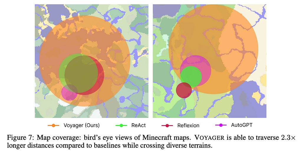
Tech progress is just one way to look at a Minecraft game. The figure below clearly outlines the parts of the game map that each LLM explored. Just look at how much further Voyager will go in the map than the others. Whether this is an accident of slightly different prompts or an inherent part of the Voyager architecture remains to be seen. As this methodology is applied to other situations we’ll have a better understanding.
This paper highlights an interesting approach to tool usage. As we push for LLMs to have greater reasoning ability, we will increasingly look for them to make decisions based on that reasoning ability. While an LLM that improves itself will be more valuable than a static one, it also poses the question: How do you make sure it doesn’t go off track?
From one point of view, this is limited to the quality of its actions. Improvement in complex environments is not always as simple as maximizing a differentiable reward function. Thus, a major area of work here will focus on validating that the LLM’s skills are improving rather than just changing.
However, from a larger point of view, we can reasonably wonder if there are some skills or areas where the LLM may become too dangerous if left to its own discretion. Areas with direct impact on human life come to mind. Now, areas like this still have problems that LLMs could solve, so the solution cannot be to freeze progress here and allow people who otherwise would have benefitted from the progress to suffer instead. Rather, we may see a world where LLMs execute the skills that humans design, creating a world that pairs human and machine intelligence.
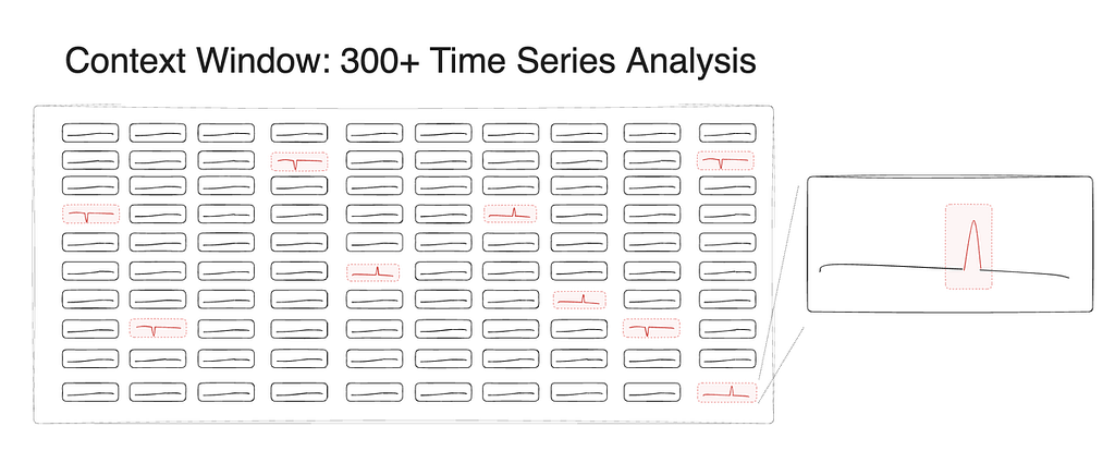
How do major LLMs stack up at detecting anomalies or movements in the data when given a large set of time series data within the context window?
While LLMs clearly excel in natural language processing tasks, their ability to analyze patterns in non-textual data, such as time series data, remains less explored. As more teams rush to deploy LLM-powered solutions without thoroughly testing their capabilities in basic pattern analysis, the task of evaluating the performance of these models in this context takes on elevated importance.
In this research, we set out to investigate the following question: given a large set of time series data within the context window, how well can LLMs detect anomalies or movements in the data? In other words, should you trust your money with a stock-picking OpenAI GPT-4 or Anthropic Claude 3 agent? To answer this question, we conducted a series of experiments comparing the performance of LLMs in detecting anomalous time series patterns.
All code needed to reproduce these results can be found in this GitHub repository.
Methodology
Figure 1: A rough sketch of the time series data (image by author)
We tasked GPT-4 and Claude 3 with analyzing changes in data points across time. The data we used represented specific metrics for different world cities over time and was formatted in JSON before input into the models. We introduced random noise, ranging from 20–30% of the data range, to simulate real-world scenarios. The LLMs were tasked with detecting these movements above a specific percentage threshold and identifying the city and date where the anomaly was detected. The data was included in this prompt template:
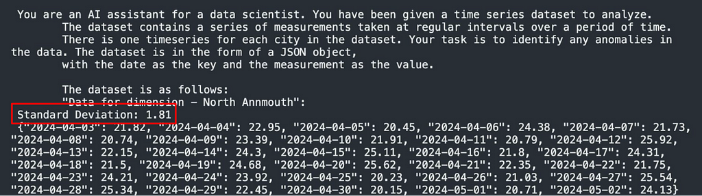
  basic template = ''' You are an AI assistant for a data scientist. You have been given a time series dataset to analyze.
  The dataset contains a series of measurements taken at regular intervals over a period of time.
  There is one timeseries for each city in the dataset. Your task is to identify anomalies in the data. The dataset is in the form of a JSON object, with the date as the key and the measurement as the value.

  The dataset is as follows:
  {timeseries_data}

  Please use the following directions to analyze the data:
  {directions}

  ...
Figure 2: The basic prompt template used in our tests
Analyzing patterns throughout the context window, detecting anomalies across a large set of time series simultaneously, synthesizing the results, and grouping them by date is no simple task for an LLM; we really wanted to push the limits of these models in this test. Additionally, the models were required to perform mathematical calculations on the time series, a task that language models generally struggle with.
We also evaluated the models’ performance under different conditions, such as extending the duration of the anomaly, increasing the percentage of the anomaly, and varying the number of anomaly events within the dataset. We should note that during our initial tests, we encountered an issue where synchronizing the anomalies, having them all occur on the same date, allowed the LLMs to perform better by recognizing the pattern based on the date rather than the data movement. When evaluating LLMs, careful test setup is extremely important to prevent the models from picking up on unintended patterns that could skew results.
Results
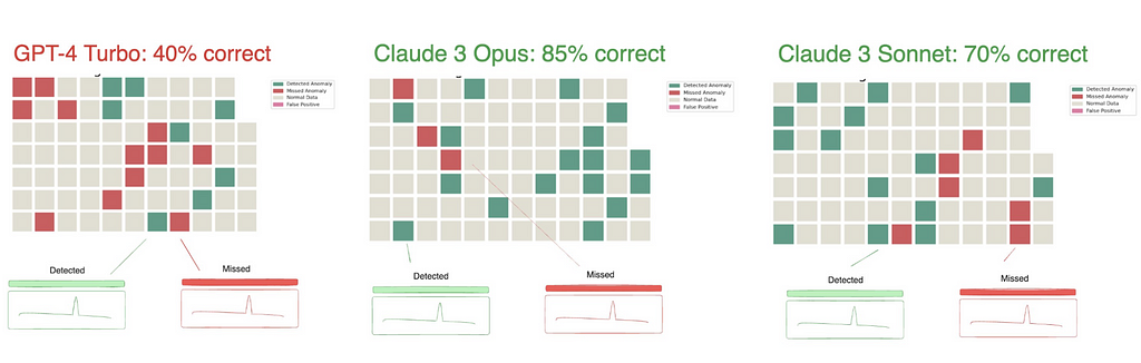
Figure 3: Claude 3 significantly outperforms GPT-4 in time series analysis (image by author)
In testing, Claude 3 Opus significantly outperformed GPT-4 in detecting time series anomalies. Given the nature of the testing, it’s unlikely that this specific evaluation was included in the training set of Claude 3 — making its strong performance even more impressive.
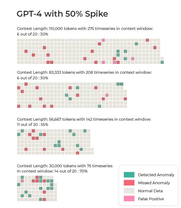
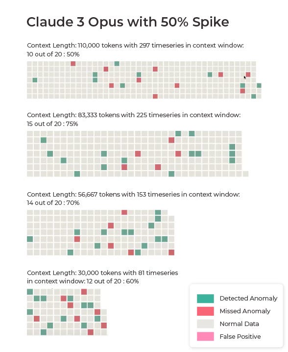
Results with 50% Spike
Our first set of results is based on data where each anomaly was a 50% spike in the data.
Figures 4a and 4b: GPT-4 and Claude 3 results with 50% spikes (images by author)
Claude 3 outperformed GPT-4 on the majority of the 50% spike tests, achieving accuracies of 50%, 75%, 70%, and 60% across different test scenarios. In contrast, GPT-4 Turbo, which we used due to the limited context window of the original GPT-4, struggled with the task, producing results of 30%, 30%, 55%, and 70% across the same tests.
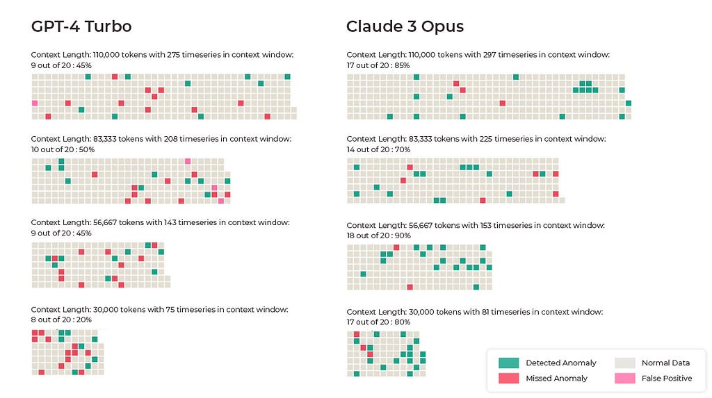
Results With 90% Spike
Claude 3’s also led where each anomaly was a 90% spike in the data.
Figure 5: ChatGPT-4 and Claude 3 results with 90% spikes
Claude 3 Opus consistently picked up the time series anomalies better than GPT-4, achieving accuracies of 85%, 70%, 90%, and 85% across different test scenarios. If we were actually trusting a language model to analyze data and pick stocks to invest in, we would of course want close to 100% accuracy. However, these results are impressive. GPT-4 Turbo’s performance ranged from 40–50% accuracy in detecting anomalies.
Results With Standard Deviation Pre-Calculated
To assess the impact of mathematical complexity on the models’ performance, we did additional tests where the standard deviation was pre-calculated and included in the data like this:
Figure 6: Standard deviation included in prompt
Since math isn’t a strong suit of large language models at this point, we wanted to see if helping the LLM complete a step of the process would help increase accuracy.
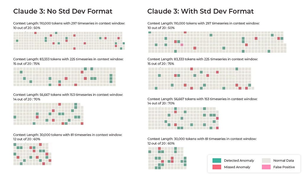
Figure 7: Standard deviation included in our prompt versus not (image by author)
The change did in fact increase accuracy across three of the four Claude 3 runs. Seemingly minor changes like this can help LLMs play to their strengths and greatly improve results.
Takeaways
This evaluation provides concrete evidence of Claude’s capabilities in a domain that requires a complex combination of retrieval, analysis, and synthesis — though the delta between model performance underscores the need for comprehensive evaluations before deploying LLMs in high-stakes applications like finance.
While this research demonstrates the potential of LLMs in time series analysis and data analysis tasks, the findings also point to the importance of careful test design to ensure accurate and reliable results — particularly since data leaks can lead to misleading conclusions about an LLM’s performance.
As always, understanding the strengths and limitations of these models is pivotal for harnessing their full potential while mitigating the risks associated with their deployment.
Bayesian sensor calibration is an emerging technique combining statistical models and data to optimally calibrate sensors — a crucial engineering procedure. This tutorial provides the Python code to perform such calibration numerically using existing libraries with a minimal math background. As an example case study, we consider a magnetic field sensor whose sensitivity drifts with temperature.
Glossary. The bolded terms are defined in the International Vocabulary of Metrology (known as the “VIM definitions”). Only the first occurrence is in bold.
Code availability. An executable Jupyter notebook for the tutorial is available on Github. It can be accessed via nbviewer.
Introduction
CONTEXT. Physical sensors provide the primary inputs that enable systems to make sense of their environment. They measure physical quantities such as temperature, electric current, power, speed, or light intensity. A measurement result is an estimate of the true value of the measured quantity (the so-called measurand). Sensors are never perfect. Non-idealities, part-to-part variations, and random noise all contribute to the sensor error. Sensor calibration and the subsequent adjustment are critical steps to minimize sensor measurement uncertainty. The Bayesian approach provides a mathematical framework to represent uncertainty. In particular, how uncertainty is reduced by “smart” calibration combining prior knowledge about past samples and the new evidence provided by the calibration. The math for the exact analytical solution can be intimidating (Berger 2022), even in simple cases where a sensor response is modeled as a polynomial transfer function with noise. Luckily, Python libraries were developed to facilitate Bayesian statistical modeling. Hence, Bayesian models are increasingly accessible to engineers. While hands-on tutorials exist (Copley 2023; Watts 2020) and even textbooks (Davidson-Pilon 2015; Martin 2021), they lack sensor calibration examples.
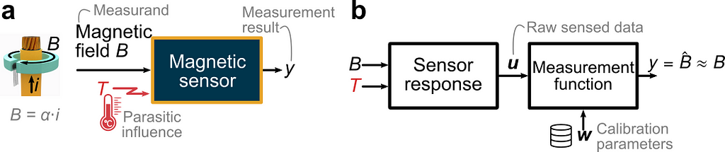
OBJECTIVE. In this article, we aim to reproduce a simplified case inspired by (Berger 2002) and illustrated in the figure below. A sensor is intended to measure the current i flowing through a wire via the measurement of the magnetic field B which is directly proportional to the current. We focus on the magnetic sensor and consider the following non-idealities. (1) The temperature B is a parasitic influence quantity disturbing the measurement. (2) The sensor response varies from one sensor to another due to part-to-part manufacturing variations. (3) The sensed data is polluted by random errors. Using a Bayesian approach and the high-level PyMC Python library, we seek to calculate the optimum set of calibration parameters for a given calibration dataset.
(a) Electric current sensor application. (b) Functional view (Image by author).
Mathematical formulation
We assume that the magnetic sensor consists of a magnetic and temperature transducer, which can be modeled as polynomial transfer functions with coefficients varying from one sensor to the next according to normal probability distributions. The raw sensed data (called “indications” in the VIM), represented by the vector u, consists of the linearly sensed magnetic field S(T)⋅B and a dimensionless sensed quantity V_T indicative of the temperature. We use the specific form S(T)⋅B to highlight that the sensitivity S is influenced by the temperature. The parasitic influence of the temperature is illustrated by the plot in panel (a) below. Ideally, the sensitivity would be independent of the temperature and of V_T. However, there is a polynomial dependency. The case study being inspired from a real magnetic Hall sensor, the sensitivity can vary by ±40% from its value at room temperature in the temperature range [−40°C, +165°C]. In addition, due to part-to-part variations, there is a set of curves S vs V_T instead of just one curve. Mathematically, we want to identify the measurement function returning an accurate estimate of the true value of the magnetic field — like shown in panel (b). Conceptually, this is equivalent to inverting the sensor response model. This boils down to estimating the temperature-dependent sensitivity and using this estimate Ŝ to recover the field from the sensed field by a division.
(a) Raw responses of N=30 sensors. (b) Block diagram (image by author).
For our simplified case, we consider that S(T) and VT(T) are second-order polynomials. The polynomial coefficients are assumed to vary around their nominal values following normal distributions. An extra random noise term is added to both sensed signals. Physically, S is the sensitivity relative to its value at room temperature, and VT is a normalized voltage from a temperature sensor. This is representative of a large class of sensors, where the primary transducer is linear but temperature-dependent, and a supplementary temperature sensor is used to correct the parasitic dependence. And both transducers are noisy. We assume that a third-order polynomial in VT is a suitable candidate for the sensitivity estimate Ŝ:
The weight vector w aggregates the 4 coefficients of the polynomial. These are the calibration parameters to be adjusted as a result of calibration.
Python formulation
We use the code convention introduced in (Close, 2021). We define a data dictionary dd to store the nominal value of the parameters. In addition, we define the probability density functions capturing the variability of the parameters. The sensor response is modeled as a transfer function, like the convention introduced in (Close 2021).
# Data dictionary: nominal parameters of the sensor response model def load_dd(): return Box({ 'S' : { 'TC' : [1, -5.26e-3, 15.34e-6], 'noise': 0.12/100, }, 'VT': { 'TC': [0, 1.16e-3, 2.78e-6], 'noise': 0.1/100,} })
# Probability density functions for the parameter variations pdfs = { 'S.TC': (norm(0,1.132e-2), norm(0,1.23e-4), norm(0,5.40e-7)), 'VT.TC' : (norm(0,7.66e-6), norm(0,4.38e-7)) }
We can then simulate a first set of N=30 sensors by drawing from the specified probability distributions, and generate synthetic data in df1 to test various calibration approaches via a build function build_sensors(ids=[..]).
df1,_=build_sensors_(ids=np.arange(30))
Synthetic data generated by the probabilistic sensor response model (Image by author).
Classic approaches
We first consider two well-known classic calibration approaches that don’t rely on the Bayesian framework.
Full regression
The first calibration approach is a brute-force approach. A comprehensive dataset is collected for each sensor, with more calibration points than unknowns. The calibration parameters w for each sensor (4 unknowns) are determined by a regression fit. Naturally, this approach provides the best results in terms of residual error. However, it is very costly in practice, as it requires a full characterization of each individual sensor. The following function performs the full calibration and store the weights as a list in the dataframe for convenience.
def full_calibration(df):
    W = df.groupby("id").apply(
        lambda g: ols("S ~ 1 + VT + I(VT**2)+ I(VT**3)", data=g).fit().params
    )
    W.columns = [f"w_{k}" for k, col in enumerate(W.columns)]
    df["w"] = df.apply(lambda X: W.loc[X.name[0]].values, axis=1)

df1, W=full_calibration(df1)
Blind calibration
A blind calibration represents the other extreme. In this approach, a first reference set of sensors is fully calibrated as above. The following sensors are not individually calibrated. Instead, the average calibration parameters w0of the reference set is reused blindly.
The following plots illustrate the residual sensitivity error Ŝ−S for the two above methods. Recall that the error before calibration reaches up to 40%. The green curves are the sensitivity error for the N=30 sensors from the reference set. Apart from a residual fourth-order error (unavoidable to the limited order of the sensitivity estimator), the fit is satisfactory (<2%). The red curve is the residual sensitivity error for ablindly calibrated sensor. Due to part-to-part variation, the average calibration parameters provide only an approximate fit, and the residual error is not satisfactory.
Residual sensitivity error for N=30 fully calibrated and N=1 blindly calibrated sensor. (Image by author).
Bayesian calibration
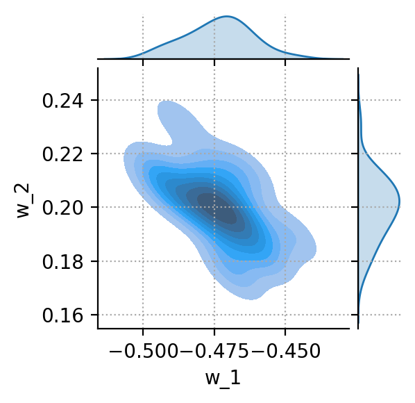
The Bayesian calibration is an interesting trade-off between the previous two extremes. A reference set of sensors is fully calibrated as above. The calibration parameters for this reference set constitute some prior knowledge. The average w0 and the covariance matrix Σ encode some relevant knowledge about the sensor response. The weights are not independent. Some combinations are more probable than others. Such knowledge should be used in a smart calibration. The coverage matrix can be calculated and plotted (for just two weights) using the Pandas and Seaborn libraries.
Bivariate plot of the two weights w_1 and w_2 (Image by author).
The Bayesian framework enables us to capture this prior knowledge, and uses it in the calibration of the subsequent samples. We restart from the same blindly calibrated samples above. We simulate the case where just two calibration data points at 0°C and 100°C are collected for each new sensor, enriching our knowledge with new evidence. In practical industrial scenarios where hardware calibration is expensive, this calibration is cost-effective. A reduced reference set is fully characterized once for all to gather prior knowledge. The subsequent samples, possibly the rest of the volume production of this batch, are only characterized at a few points. In Bayesian terminology, this is called “inference”, and the PyMC library provides high-level functions to perform inference. It is a computation-intensive process because the posterior distribution, which is obtained by applying the Bayes’ theorem combining the prior knowledge and the new evidence, can only be sampled. There is no analytical approximation of the obtained probability density function.
The calibration results are compared below, with the blue dot indicating the two calibration points used by the Bayesian approach. With just two extra points and by exploiting the prior knowledge acquired on the reference set, the Bayesian calibrated sensor exhibits an error hardly degraded compared to the expensive brute-force approach.
Comparison of the three calibration approaches.
Credible interval
In the Bayesian approach, all variables are characterized by uncertainty in. The parameters of the sensor model, the calibration parameters, but also the posterior predictions. We can then construct a ±1σ credible interval covering 68% of the synthetic observations generated by the model for the estimated sensitivity Ŝ. This plot captures the essence of the calibration and adjustment: the uncertainty has been reduced around the two calibration points at T=0°C and T=100°C. The residual uncertainty is due to noisy measurements.
Credible interval (Image by author).
Conclusion
This article presented a Python workflow for simulating Bayesian sensor calibration, and compared it against well-known classic approaches. The mathematical and Python formulations are valid for a wide class of sensors, enabling sensor design to explore various approaches. The workflow can be summarized as follows:
Model the sensor response in terms of transfer function and the parameters (nominal values and statistical variations). Generate corresponding synthetic raw sensed data for a batch of sensors.
Define the form of the measurement function from the raw sensed variables. Typically, this is a polynomial, and the calibration should determine the optimum coefficients w of this polynomial for each sensor.
Acquire some prior knowledge by fully characterizing a representative subset of sensors. Encode this knowledge in the form of average calibration parameters and covariance matrix.
Acquire limited new evidence in the form of a handful of calibration points specific to each sensor.
Perform Bayesian inference merging this new sparse evidence with the prior knowledge to find the most likely calibration parameters for this new sensor numerically using PyMC.
In the frequent cases where sensor calibration is a significant factor of the production cost, Bayesian calibration exhibits substantial business benefits. Consider a batch of 1’000 sensors. One can obtain representative prior knowledge with a full characterization from, say, only 30 sensors. And then for the other 970 sensors, use a few calibration points only. In a classical approach, these extra calibration points lead to an undetermined system of equations. In the Bayesian framework, the prior knowledge fills the gap.
We use cookies on our website to give you the most relevant experience by remembering your preferences and repeat visits. By clicking “Accept”, you consent to the use of ALL the cookies.
This website uses cookies to improve your experience while you navigate through the website. Out of these, the cookies that are categorized as necessary are stored on your browser as they are essential for the working of basic functionalities of the website. We also use third-party cookies that help us analyze and understand how you use this website. These cookies will be stored in your browser only with your consent. You also have the option to opt-out of these cookies. But opting out of some of these cookies may affect your browsing experience.
Necessary cookies are absolutely essential for the website to function properly. These cookies ensure basic functionalities and security features of the website, anonymously.
Cookie
Duration
Description
cookielawinfo-checkbox-analytics
11 months
This cookie is set by GDPR Cookie Consent plugin. The cookie is used to store the user consent for the cookies in the category "Analytics".
cookielawinfo-checkbox-functional
11 months
The cookie is set by GDPR cookie consent to record the user consent for the cookies in the category "Functional".
cookielawinfo-checkbox-necessary
11 months
This cookie is set by GDPR Cookie Consent plugin. The cookies is used to store the user consent for the cookies in the category "Necessary".
cookielawinfo-checkbox-others
11 months
This cookie is set by GDPR Cookie Consent plugin. The cookie is used to store the user consent for the cookies in the category "Other.
cookielawinfo-checkbox-performance
11 months
This cookie is set by GDPR Cookie Consent plugin. The cookie is used to store the user consent for the cookies in the category "Performance".
viewed_cookie_policy
11 months
The cookie is set by the GDPR Cookie Consent plugin and is used to store whether or not user has consented to the use of cookies. It does not store any personal data.
Functional cookies help to perform certain functionalities like sharing the content of the website on social media platforms, collect feedbacks, and other third-party features.
Performance cookies are used to understand and analyze the key performance indexes of the website which helps in delivering a better user experience for the visitors.
Analytical cookies are used to understand how visitors interact with the website. These cookies help provide information on metrics the number of visitors, bounce rate, traffic source, etc.
Advertisement cookies are used to provide visitors with relevant ads and marketing campaigns. These cookies track visitors across websites and collect information to provide customized ads.