We are excited to announce the general availability of two advanced recipes in Amazon Personalize, User-Personalization-v2 and Personalized-Ranking-v2 (v2 recipes), which are built on the cutting-edge Transformers architecture to support larger item catalogs with lower latency. In this post, we summarize the new enhancements, and guide you through the process of training a model and providing recommendations for your users.
Embeddings are integral to various natural language processing (NLP) applications, and their quality is crucial for optimal performance. They are commonly used in knowledge bases to represent textual data as dense vectors, enabling efficient similarity search and retrieval. In Retrieval Augmented Generation (RAG), embeddings are used to retrieve relevant passages from a corpus to provide […]
Some months, our community appears to be drawn to a very tight cluster of topics: a new model or tool pops up, and everyone’s attention zooms in on the latest, buzziest news. Other times, readers seem to be moving in dozens of different directions, diving into a wide spectrum of workflows and themes. Last month definitely belongs to the latter camp, and as we looked at the articles that resonated the most with our audience, we were struck (and impressed!) by their diversity of perspectives and focal points.
We hope you enjoy this selection of some of our most-read, -shared, and -discussed posts from April, which include a couple of this year’s most popular articles to date, and several top-notch (and beginner-friendly) explainers.
Monthly Highlights
The Math Behind Neural Networks By now, few of you need an introduction to Cristian Leo’s series of guides to the essential concepts of machine learning. Perhaps none of these building blocks are more essential than neural networks, of course, so it comes as no surprise that this deep dive into their underlying math became such a success among our readers.
Pandas: From Messy To Beautiful It’s always a joy to see an author’s first TDS article strike a chord with a wide audience; this is precisely what happened with Anna Zawadzka’s practical guide to improving your Pandas code, providing actionable tips for keeping it “clean and infallible.”
A New Coefficient of Correlation True breakthroughs in statistics don’t arrive very often these days—which explains why Tim Sumner’s article on a recent paper, which introduced a “new way to measure the relationship between two variables just like correlation except possibly better,” generated a massive response from data professionals.
How to Build a Local Open-Source LLM Chatbot With RAG Several months after making their initial splash in ML circles, RAG approaches seem to have lost none of their shine. Dr. Leon Eversberg’s tutorial is a case in point: it adds a novel solution to a growing list of tools that allow us to “talk” to our PDF documents.
Deep Dive into Transformers by Hand Transformers guides and technical walkthroughs aren’t exactly hard to find. What sets Srijanie Dey, PhD’s contribution apart is its accessibility and clarity —which, along with its well-executed illustrations, made it a particularly strong resource for beginners and visual learners.
From Data Scientist to ML / AI Product Manager Making a career transition is never a trivial endeavor, and even less so during a difficult period for job seekers. Anna Via offered a generous dose of inspiration, along with more than a few actionable tips and insights, based on her own successful role switch to become a machine learning product manager.
The 4 Hats of a Full-Stack Data Scientist What does it take to become a genuine “full-stack” data professional? Shaw Talebi recently launched a series exploring (and answering) this question in detail; this post, the first in the sequence, provides a high-level perspective into the core skills of a data scientist who can “see the big picture and dive into specific aspects of a project as needed.”
Meet the NiceGUI: Your Soon-to-be Favorite Python UI Library It’s tough to keep track of all the exciting new libraries, packages, and platforms announced every day—which is why a detailed, opinionated, firsthand review can be so useful. That’s precisely what Youness Mansar sets out to accomplish with his intro to NiceGUI, an open-source Python-based UI framework.
Linear Regressions for Causal Conclusions More often than not, keeping things simple is the key to success. That’s a point that Mariya Mansurova drives home again and again in her guide to drawing causal conclusions in the context of product analytics, which avoids fancy algorithms and complex equations in favor of tried-and-true linear regressions.
Thank you for supporting the work of our authors! We love publishing articles from new authors, so if you’ve recently written an interesting project walkthrough, tutorial, or theoretical reflection on any of our core topics, don’t hesitate to share it with us.
My students and I measuring the retreat of the Cotopaxi glacier.
I was born and raised in Ecuador. In this country, weather and climate shape our lives. For example, our energy supply relies on sufficient rainfall for hydroelectric power. As a child, I remember having continuous blackouts. Unfortunately, Ecuador has not been resilient. At the time of writing this article, we are experiencing blackouts again. Paradoxically, El Niño Southern Oscillation brings us flooding every year. I love hiking, and with great sadness, I saw how our glaciers have retreated.
Ten years ago, I decided to study for a PhD in meteorology. Climate change and its implications troubled me. It is a daunting challenge that humanity faces in this century. There has been enormous progress in our scientific understanding of this problem. But we still need more action.
When I started my PhD, few researchers used artificial intelligence (AI) techniques. Nowadays, there is a consensus that harnessing the potential of AI can make a difference. In particular, in mitigating and adapting to climate change.
ML and in particular computer vision (CV) empower us to make sense of the massive amounts of available data. This power will allow us to take action. Uncovering hidden patterns in visual data (eg. satellite data) is a critical task in tackling climate change.
This article introduces CV and its intersection with climate change. It is the first of a series on this topic. The article has five sections. First, it presents an introduction. Next, the article defines some basic concepts related to CV. Then, it explores the capabilities of CV to tackle climate change with case studies. After that, the article discusses challenges and future directions. Finally, a summary provides an overview.
Understanding Computer Vision
CV uses computational methods to learn patterns from images. Earth Observation (EO) relies mainly on satellite images. Thus, CV is a well-suited tool for climate change analysis. To understand climate patterns from images, several techniques are necessary. Some of the most important are classification, object detection, and segmentation.
Classification: involves categorizing (single) images based on predefined classes (single labels). Fire detection and burned area mapping use image classification techniques on satellite images. These images provide spectral signatures linked to burned vegetation. Using these unique patterns researchers can track the impact of wildfires.
Object detection: comprises locating objects in an area of interest. The track of hurricanes and cyclones uses this technique. Detecting its cloud patterns helps to mitigate their impact in coastal zones.
Image segmentation: assigns a class to each pixel in an image. This technique helps to identify regions and their boundaries. Segmentation is also referred to as “semantic segmentation”. Since each region (target class) receives a label its definition includes “semantic”. For example, tracking a glacier’s retreat uses this technique. Segmenting satellite images from glaciers allows for tracking their changes. For instance, monitoring glacier’s extent, area, and volume over time.
This section provided some examples of CV in action to tackle climate change. The following section will analyze them as case studies.
Case Study 1: Wildfire detection
Credit: Issy Bailey (Unsplash)
Climate change has several implications for wildfires. For example, increasing the likelihood of extreme events. Also, extending the timeframe of fire seasons. Likewise, it will exacerbate fire intensity. Thus, investing resources in innovative solutions to prevent catastrophic wildfires is imperative.
This type of research depends on the analyses of images for early detection of wildfires. ML methods, in general, proved to be effective in predicting these events.
However, advanced AI deep learning algorithms yield the best results. An example of these advanced algorithms is Neural Networks (NNs). NNs are an ML technique inspired by human cognition. This technique relies on one or more convolutional layers to detect features.
Convolutional Neural Networks (CNN) are popular in Earth Science applications. CNN shows the greatest potential to increase the accuracy of fire detection. Several models use this algorithm, such as VGGNet, AlexNet, or GoogleNet. These models present improved accuracy in CV tasks.
Fire detection through CV algorithms requires image segmentation. Yet, before segmenting the data, it needs preprocessing. For instance, to reduce noise, normalize values, and resize. Next, the analysis labels pixels that represent fire. Thus distinguishing them from other image information.
Case Study 2: Cyclone Tracking
Credit:NASA (Unsplash)
Climate change will increase the frequency and intensity of cyclones. In this case, a massive amount of data is not processed by real-time applications. For instance, data from models, satellites, radar, and ground-based weather stations. CV demonstrates to be efficient in processing these data. It has also reduced the biases and errors linked with human intervention.
For example, numerical weather prediction models use only 3%–7% of data. In this case, observations from Geostationary Operational Environmental Satellites (GOES). The data assimilation processes use even less of these data. CNN models select among this vast quantity of images the most relevant observations. These observations refer to cyclone-active (or soon-to-be active) regions of interest (ROI).
Identifying this ROI is a segmentation task. There are several models used in Earth Sciences to approach this problem. Yet, the U-Net CNN is one of the most popular choices. The model design relates to medical segmentation tasks. But it has proven useful in solving meteorological problems as well.
Case Study 3:Tracking Glacial Retreat
Credit: Ryan Stone (Unsplash)
Glaciers are thermometers of climate change. The effects of climate variations on glaciers are visual (retreat of outlines). Thus, they symbolize the consequences of climate variability and change. Besides the visual impacts, the glacier retreat has other consequences. For example, adverse effects on water resource sustainability. Destabilization of hydropower generation. Affecting drinking water quality. Reductions in agricultural production. Unbalancing ecosystems. On a global scale, even the increase in sea level threatens coastal regions.
The process of monitoring glaciers used to be time-consuming. The interpretation of satellite images needs experts to digitalize and analyze them. CV can help to automate this process. Additionally, computer vision can make the process more efficient. For example, allowing the incorporation of more data into the modeling. CNN models such as GlacierNet harness the power of deep learning to track glaciers.
There are several techniques to detect glacier boundaries. For example, segmentation, object detection, and also edge detection. CV can perform even more complex tasks. Comparing glacier images over time is one example. Likewise, determining the velocity of movement of glaciers and even their thickness. These are powerful tools to track glacier dynamics. These processes can extract valuable information for adaptation purposes.
Challenges and Future Directions
There are particular challenges in tackling climate change using CV. Discussing each of them may need an entire book. However, the aim here is modest. I will attempt to bring them to the table for a reference.
Data complexity: The need, and the inherent complexity, of using many sources of data. For example, satellite and aerial imagery, lidar data, and ground-based sensors. Data fusion is an evolving technique that attempts to address this challenging issue.
Model interpretability: a current challenge is developing hybrid models. It means reconciling a statistical data-driven model with a physical one. The interpretability of CV algorithms increases incorporating our knowledge of the climate system. Thus, these models excel in fitting complex functions. But also should provide an understanding of the underlying causal relations.
Labeled samples: The availability of high-quality labeled samples. These samples should be specific to EO problems to train CV models. Generating them is a time-consuming and costly task. Addressing this challenge is an active area of research.
Ethics: Is a challenge to incorporate ethical considerations in AI development. Privacy, fairness, and accountability play a key role in ensuring trust with stakeholders. Considering environmental justice is also a sound strategy in the context of climate change.
Summary
CV is a powerful tool to tackle climate change. From detecting wildfires to tracking cyclone formation and glacier retreats. CV is transforming how to monitor, predict, and project climate impacts. The study of these impacts relies on CV techniques. For example, classification, object detection, and segmentation. Finally, several challenges arise in the intersection between CV and climate change. For instance, managing multiple sources of data. Enhancing the interpretability of machine learning models. Generating high-quality labeled samples to train CV models. And incorporating ethical considerations when designing an AI system. A subsequent article will present a guide to collecting and curating image datasets. In particular, those relevant to climate change.
References
Kumler-Bonfanti, C., Stewart, J., Hall, D., & Govett, M. (2020). Tropical and extratropical cyclone detection using deep learning. Journal of Applied Meteorology and Climatology, 59(12), 1971–1985.
Maslov, K. A., Persello, C., Schellenberger, T., & Stein, A. (2024). Towards Global Glacier Mapping with Deep Learning and Open Earth Observation Data. arXiv preprint arXiv:2401.15113.
Moumgiakmas, S. S., Samatas, G. G., & Papakostas, G. A. (2021). Computer vision for fire detection on UAVs — From software to hardware. Future Internet, 13(8), 200.
Rolnick, D., Donti, P. L., Kaack, L. H., Kochanski, K., Lacoste, A., Sankaran, K., … & Bengio, Y. (2022). Tackling climate change with machine learning. ACM Computing Surveys (CSUR), 55(2), 1–96.
Tuia, D., Schindler, K., Demir, B., Camps-Valls, G., Zhu, X. X., Kochupillai, M., … & Schneider, R. (2023). Artificial intelligence to advance Earth observation: a perspective. arXiv preprint arXiv:2305.08413.
Window functions are key to writing SQL code that is both efficient and easy to understand. Knowing how they work and when to use them will unlock new ways of solving your reporting problems.
The objective of this article is to explain window functions in SQL step by step in an understandable way so that you don’t need to rely on only memorizing the syntax.
Here is what we will cover:
An explanation on how you should view window functions
Go over many examples in increasing difficulty
Look at one specific real-case scenario to put our learnings into practice
Review what we’ve learned
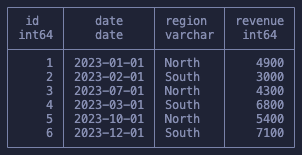
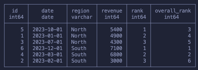
Our dataset is simple, six rows of revenue data for two regions in the year 2023.
Window Functions Are Sub Groups
If we took this dataset and ran a GROUP BY sum on the revenue of each region, it would be clear what happens, right? It would result in only two remaining rows, one for each region, and then the sum of the revenues:
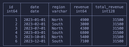
The way I want you to view window functions is very similar to this but, instead of reducing the number of rows, the aggregation will run “in the background” and the values will be added to our existing rows.
First, an example:
SELECT
 id,
    date,
    region,
    revenue,
    SUM(revenue) OVER () as total_revenue
FROM
    sales
Notice that we don’t have any GROUP BY and our dataset is left intact. And yet we were able to get the sum of all revenues. Before we go more in depth in how this worked let’s just quickly talk about the full syntax before we start building up our knowledge.
The Window Function Syntax
The syntax goes like this:
SUM([some_column]) OVER (PARTITION BY [some_columns] ORDER BY [some_columns])
Picking apart each section, this is what we have:
An aggregation or window function: SUM, AVG, MAX, RANK, FIRST_VALUE
The OVER keyword which says this is a window function
The PARTITION BY section, which defines the groups
The ORDER BY section which defines if it’s a running function (we will cover this later on)
Don’t stress over what each of these means yet, as it will become clear when we go over the examples. For now just know that to define a window function we will use the OVER keyword. And as we saw in the first example, that’s the only requirement.
Building Our Understanding Step By Step
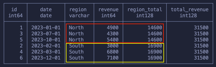
Moving to something actually useful, we will now apply a group in our function. The initial calculation will be kept to show you that we can run more than one window function at once, which means we can do different aggregations at once in the same query, without requiring sub-queries.
SELECT
    id,
    date,
    region,
    revenue,
    SUM(revenue) OVER (PARTITION BY region) as region_total,
    SUM(revenue) OVER () as total_revenue
FROM sales
As said, we use the PARTITION BY to define our groups (windows) that are used by our aggregation function! So, keeping our dataset intact we’ve got:
The total revenue for each region
The total revenue for the whole dataset
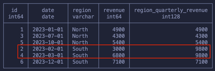
We’re also not restrained to a single group. Similar to GROUP BY we can partition our data on Region and Quarter, for example:
SELECT
    id,
    date,
    region,
    revenue,
    SUM(revenue) OVER (PARTITION BY
          region,
          date_trunc('quarter', date)
    ) AS region_quarterly_revenue
FROM sales
In the image we see that the only two data points for the same region and quarter got grouped together!
At this point I hope it’s clear how we can view this as doing a GROUP BY but in-place, without reducing the number of rows in our dataset. Of course, we don’t always want that, but it’s not that uncommon to see queries where someone groups data and then joins it back in the original dataset, complicating what could be a single window function.
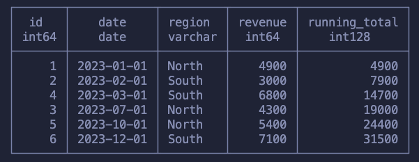
Moving on to the ORDER BY keyword. This one defines a running window function. You’ve probably heard of a Running Sum once in your life, but if not, we should start with an example to make everything clear.
SELECT
    id,
    date,
    region,
    revenue,
    SUM(revenue) OVER (ORDER BY id) as running_total
FROM sales
What happens here is that we’ve went, row by row, summing the revenue with all previous values. This was done following the order of the id column, but it could’ve been any other column.
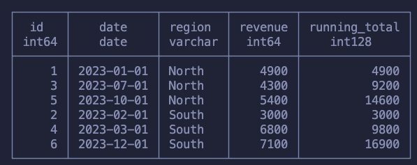
This specific example is not particularly useful because we’re summing across random months and two regions, but using what we’ve learned we can now find the cumulative revenue per region. We do that by applying the running sum within each group.
SELECT
    id,
    date,
    region,
    revenue,
    SUM(revenue) OVER (PARTITION BY region ORDER BY date) as running_total
FROM sales
Take the time to make sure you understand what happened here:
For each region we’re walking up month by month and summing the revenue
Once it’s done for that region we move to the next one, starting from scratch and again moving up the months!
It’s quite interesting to notice here that when we’re writing these running functions we have the “context” of other rows. What I mean is that to get the running sum at one point, we must know the previous values for the previous rows. This becomes more obvious when we learn that we can manually chose how many rows before/after we want to aggregate on.
SELECT
    id,
    date,
    region,
    revenue,
    SUM(revenue) OVER (ORDER BY id ROWS BETWEEN 1 PRECEDING AND 2 FOLLOWING)
    AS useless_sum
FROM
    sales
For this query we specified that for each row we wanted to look at one row behind and two rows ahead, so that means we get the sum of that range! Depending on the problem you’re solving this can be extremely powerful as it gives you complete control on how you’re grouping your data.
Finally, one last function I want to mention before we move into a harder example is the RANK function. This gets asked a lot in interviews and the logic behind it is the same as everything we’ve learned so far.
SELECT
    *,
    RANK() OVER (PARTITION BY region ORDER BY revenue DESC) as rank,
    RANK() OVER (ORDER BY revenue DESC) as overall_rank
FROM
    sales
ORDER BY region, revenue DESC
Just as before, we used ORDER BY to specify the order which we will walk, row by row, and PARTITION BY to specify our sub-groups.
The first column ranks each row within each region, meaning that we will have multiple “rank one’s” in the dataset. The second calculation is the rank across all rows in the dataset.
Forward Filling Missing Data
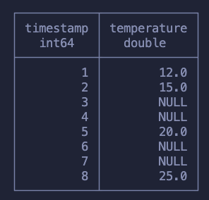
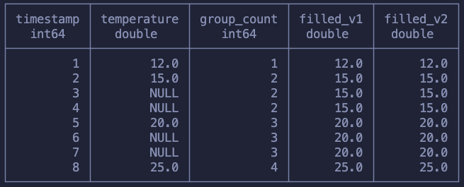
This is a problem that shows up every now and then and to solve it on SQL it takes heavy usage of window functions. To explain this concept we will use a different dataset containing timestamps and temperature measurements. Our goal is to fill in the rows missing temperature measurements with the last measured value.
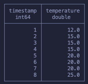
Here is what we expect to have at the end:
Before we start I just want to mention that if you’re using Pandas you can solve this problem simply by running df.ffill() but if you’re on SQL the problem gets a bit more tricky.
The first step to solve this is to, somehow, group the NULLs with the previous non-null value. It might not be clear how we do this but I hope it’s clear that this will require a running function. Meaning that it’s a function that will “walk row by row”, knowing when we hit a null value and when we hit a non-null value.
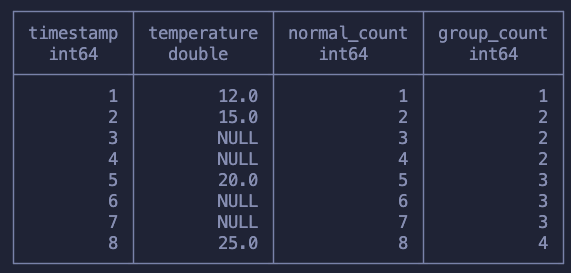
The solution is to use COUNT and, more specifically, count the values of temperature measurements. In the following query I run both a normal running count and also a count over the temperature values.
SELECT
    *,
    COUNT() OVER (ORDER BY timestamp) as normal_count,
    COUNT(temperature) OVER (ORDER BY timestamp) as group_count
from sensor
In the first calculation we simply counted up each row increasingly
On the second one we counted every value of temperature we saw, not counting when it was NULL
The normal_count column is useless for us, I just wanted to show what a running COUNT looked like. Our second calculation though, the group_count moves us closer to solving our problem!
Notice that this way of counting makes sure that the first value, just before the NULLs start, is counted and then, every time the function sees a null, nothing happens. This makes sure that we’re “tagging” every subsequent null with the same count we had when we stopped having measurements.
Moving on, we now need to copy over the first value that got tagged into all the other rows within that same group. Meaning that for the group 2 needs to all be filled with the value 15.0.
Can you think of a function now that we can use here? There is more than one answer for this, but, again, I hope that at least it’s clear that now we’re looking at a simple window aggregation with PARTITION BY .
SELECT
    *,
    FIRST_VALUE(temperature) OVER (PARTITION BY group_count) as filled_v1,
    MAX(temperature) OVER (PARTITION BY group_count) as filled_v2
FROM (
    SELECT
        *,
        COUNT(temperature) OVER (ORDER BY timestamp) as group_count
    from sensor
) as grouped
ORDER BY timestamp ASC
We can use both FIRST_VALUE or MAX to achieve what we want. The only goal is that we get the first non-null value. Since we know that each group contains one non-null value and a bunch of null values, both of these functions work!
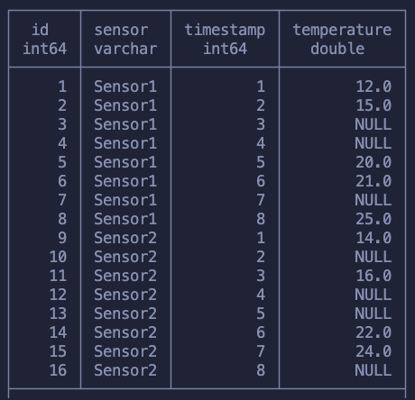
This example is a great way to practice window functions. If you want a similar challenge try to add two sensors and then forward fill the values with the previous reading of that sensor. Something similar to this:
Could you do it? It doesn’t use anything that we haven’t learned here so far.
By now we know everything that we need about how window functions work in SQL, so let’s just do a quick recap!
Recap Time
This is what we’ve learned:
We use the OVER keyword to write window functions
We use PARTITION BY to specify our sub-groups (windows)
If we provide only the OVER() keyword our window is the whole dataset
We use ORDER BY when we want to have a running function, meaning that our calculation walks row by row
Window functions are useful when we want to group data to run an aggregation but we want to keep our dataset as is
I hope this helped you understand how window functions work and helps you apply it in the problems you need to solve.
When we think of algorithms, we often describe them as similar to a recipe: a series of steps we follow to complete some task. We frequently use that definition when writing code, breaking down what must be done into smaller steps and writing code that executes them.
Although that intuitive notion of algorithm serves us well most of the time, having a formal definition allows us to do even more. With it, we can prove that some problems are fundamentally unsolvable, have a common ground for comparing and analyzing algorithms, and develop new ones. Nowadays, the Turing Machine is what typically fills that spot.
The Birth of the Turing Machine
Until the beginning of the 20th century, even mathematicians didn’t have a formal definition of what an algorithm was. Much like most of us do today, they relied on that same intuitive concept: a finite number of steps by which a function could be effectively calculated.
This became a limiting factor for mathematics in the last century. In 1928, David Hilbert, alongside Wilhelm Ackermann, proposed the decision problem, or the Entscheidungsproblem in German. The problem went as follows:
Is there an algorithm that can definitely answer “yes” or “no” to any mathematical statement?
This question couldn’t be answered without a proper definition of algorithm. Even before this, in 1900, Hilbert had also proposed 23 problems as challenges for the century to come, one of which ran into the same issue. The lack of a formal notion had already been plaguing mathematicians for a while.
Around 1936, two separate solutions to the Entscheidungsproblem were published independently. To solve it, they each proposed a method for how to define an algorithm. Alan Turing gave birth to the Turing Machine and Alonzo Church invented λ-Calculus. Both reached the same conclusion: the algorithm hypothesized by Hilbert and Ackermann couldn’t exist.
The two descriptions were equivalent in terms of power. That is, anything that could be described by a Turing machine could be described by λ-calculusand vice-versa. We tend to prefer Turing’s definition when discussing computer theory but assume both to be perfectly sufficient methods of describing an algorithm. This is known as the Church-Turing thesis.
A function can only be calculated by an effective method if it is computable by a Turing machine (or λ-calculus).
How Turing Machines Work
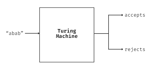
In simple terms, one can think of a Turing machine as a black box that receives a string of characters, processes it in some way, and returns whether it either accepts or denies the input.
A black-box diagram of a Turing machine. Image by author.
This may seem strange at first, but it’s common in low-level languages like C, C++, or even bash script. When writing code in one of these languages, we often return 0 at the end of our script to signify a successful execution. We may have it instead return a 1 in case of a generic error.
#include <stdio.h>

int main()
{
  printf("Hello World!");
  return 0;
}
These values can then be checked by the operating system or other programs. Programming languages also allow for the return of numbers greater than 1 to specify a particular type of error but the general gist is still the same. As for what it means for a machine to accept or reject a certain input, that’s entirely up to the one who designed it.
Behind the curtain, the machine is made up of two core components: a control block and a tape. The tape is infinite and corresponds to the model’s memory. The control block can interact with the tape through a moving head that can both read from and write into the tape. The head can move left and right across the tape. It can go infinitely into the right but can’t go further left than the tape’s starting element as the tape only expands indefinitely towards one side.
A simplified diagram of the Turing machine. Image by author.
At first, the tape is empty, filled only with blank symbols (⊔). When the machine reads the input string, it gets placed at the leftmost part of the tape. The head is also moved to the leftmost position, allowing the machine to start reading the input sequence from there. How it goes about reading the input, whether it writes over it, and any other implementation details are defined in the control block.
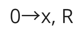
The control block is made up of a set of states interconnected by a transition function. The transitions defined in the transition function specify how to move between states depending on what is read from the tape, as well as what to write onto it and how to move its head.
A single transition in a Turing machine. Image by author.
In the transition above, the first term refers to what is being read from the tape. Following the arrow, the next term will be written on the tape. Not only does the tape allow for any of the characters in the input to be written on it, but it also permits the usage of additional symbols present only in the tape. Following the comma, the last term is the direction in which to move the head: R means right and L means left.
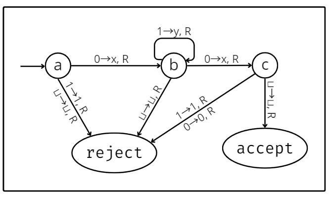
The diagram below describes the inner workings of a Turing machine that accepts any string of at least 2 in length that starts and ends with 0, with an arbitrary amount of 1s in the middle. The transitions are placed next to arrows that point from one state to another. Every time the machine reads a character from the tape, it will check all the transitions that leave its current state. Then, it transitions along the arrow containing that symbol into the next state.
State diagram for a Turing machine that accepts L = 01*0 (1* means a series of n 1s, where n ≥ 0). Image by author.
The Turing machine has 3 special states: a starting, an acceptance, and a rejection state. The starting state is indicated in the diagram by an arrow that only connects on one end and, as the name suggests, is the state the machine starts in. The remaining 2 states are equally straightforward: if the machine reaches the acceptance state, it accepts the input, and if it reaches the rejection state, it rejects it. Note that it may also loop eternally, without ever reaching either of them.
The diagram used was one for a deterministic Turing machine. That means every state had a transition leaving it for every possible symbol it may have read from the tape. In a non-deterministic Turing machine, this wouldn’t be the case. It is one of many Turing machine variations. Some may adopt more than one tape, others may have a “printer” attached, etc. The one thing to keep in mind with variations of the model is that they’re all equivalent in terms of power. That is, anything that any Turing machine variation can compute can also be calculated by the deterministic model.
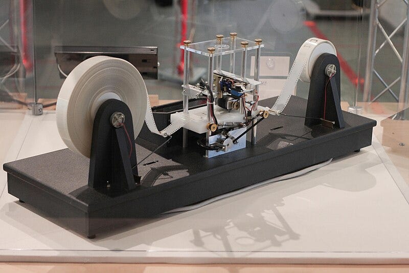
The picture below is of a simple physical model of a Turing machine built by Mike Davey. It has a tape that can be moved left or right by two rotating motors and at its center lies a circuit that can read from and write onto the tape, perfectly capturing Turing’s concept.
Despite being simple, Turing machines are mighty. As the modern definition of an algorithm, it boasts the power to compute anything a modern computer can. After all, modern computers are based on the same principles. One might even refer to them as highly sophisticated real-world implementations of Turing machines.
That said, the problems dealt with by modern computers and the data structures used to tackle them are often much more complex than what we’ve discussed. How do Turing machines solve these problems? The trick behind it is encoding. No matter how complex, any data structure can be represented as a simple string of characters.
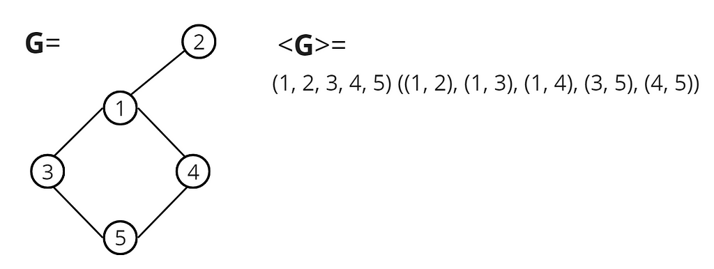
An undirected graph G and its encoding <G>. Image by author.
In the example above, we represent an undirected connected graph as a list of nodes followed by a list of edges. We use parenthesis and commas to isolate the individual nodes and edges. As long as the algorithm implemented by the Turing machine considers this representation, it should be able to perform any graph-related computations done by modern computers.
Data structures are stored in much the same way in real computers — just strings consisting of ones and zeros. In the end, at the barest level, all modern computers do is read and write strings of bits from and onto memory while following some logic. And, in doing so, they allow us to solve all kinds of problems from the barest to the highest complexity.
Conclusion
Understanding Turing machines and how they work provides helpful insight into the capabilities and limitations of computers. Beyond giving us a solid theoretical foundation to understand the underpinnings of complex algorithms, it allows us to determine whether an algorithm can even solve a given problem in the first place.
They are also central to complexity theory, which studies the difficulty of computational problems and how many resources, like time or memory, are required to solve them. Analyzing the complexity of an algorithm is an essential skill for anyone who works with software. Not only does it allow for the development of more efficient models and algorithms, as well as the optimization of existing ones, but it’s also helpful in choosing the right algorithm for the job.
In conclusion, a deep comprehension of Turing machines not only grants us a profound understanding of computers’ capabilities and boundaries but also gives us the foundation and tools necessary to ensure the efficiency of our solutions and drive innovation forward.
Large language models (LLMs) are making a significant impact in the realm of artificial intelligence (AI). Their impressive generative abilities have led to widespread adoption across various sectors and use cases, including content generation, sentiment analysis, chatbot development, and virtual assistant technology. Llama2 by Meta is an example of an LLM offered by AWS. Llama […]
Imagine harnessing the power of advanced language models to understand and respond to your customers’ inquiries. Amazon Bedrock, a fully managed service providing access to such models, makes this possible. Fine-tuning large language models (LLMs) on domain-specific data supercharges tasks like answering product questions or generating relevant content. In this post, we show how Amazon […]
Organizations often offer support in multiple languages, saying “contact us for translations.” However, customers who don’t speak the predominant language often don’t know that translations are available or how to request them. This can lead to poor customer experience and lost business. A better approach is proactively providing information in multiple languages so customers can […]
We use cookies on our website to give you the most relevant experience by remembering your preferences and repeat visits. By clicking “Accept”, you consent to the use of ALL the cookies.
This website uses cookies to improve your experience while you navigate through the website. Out of these, the cookies that are categorized as necessary are stored on your browser as they are essential for the working of basic functionalities of the website. We also use third-party cookies that help us analyze and understand how you use this website. These cookies will be stored in your browser only with your consent. You also have the option to opt-out of these cookies. But opting out of some of these cookies may affect your browsing experience.
Necessary cookies are absolutely essential for the website to function properly. These cookies ensure basic functionalities and security features of the website, anonymously.
Cookie
Duration
Description
cookielawinfo-checkbox-analytics
11 months
This cookie is set by GDPR Cookie Consent plugin. The cookie is used to store the user consent for the cookies in the category "Analytics".
cookielawinfo-checkbox-functional
11 months
The cookie is set by GDPR cookie consent to record the user consent for the cookies in the category "Functional".
cookielawinfo-checkbox-necessary
11 months
This cookie is set by GDPR Cookie Consent plugin. The cookies is used to store the user consent for the cookies in the category "Necessary".
cookielawinfo-checkbox-others
11 months
This cookie is set by GDPR Cookie Consent plugin. The cookie is used to store the user consent for the cookies in the category "Other.
cookielawinfo-checkbox-performance
11 months
This cookie is set by GDPR Cookie Consent plugin. The cookie is used to store the user consent for the cookies in the category "Performance".
viewed_cookie_policy
11 months
The cookie is set by the GDPR Cookie Consent plugin and is used to store whether or not user has consented to the use of cookies. It does not store any personal data.
Functional cookies help to perform certain functionalities like sharing the content of the website on social media platforms, collect feedbacks, and other third-party features.
Performance cookies are used to understand and analyze the key performance indexes of the website which helps in delivering a better user experience for the visitors.
Analytical cookies are used to understand how visitors interact with the website. These cookies help provide information on metrics the number of visitors, bounce rate, traffic source, etc.
Advertisement cookies are used to provide visitors with relevant ads and marketing campaigns. These cookies track visitors across websites and collect information to provide customized ads.