A user guide to mapping golf courses in Google Earth and bringing them to life in R.
In the land of data viz, we are often inundated with bar, line, and pie charts. But it doesn’t have to be that way — in this article, I will demonstrate how to plot golf courses.
Image by the author
Introduction
There are close to 40,000 golf courses worldwide. If you are passionate about golf and/or data like I am then this is for you. After plotting a course, there are some other cool things we can do as well:
Overlaying shots onto course map — this can be donewith some manipulation using the Plotly package, or by downloading individual golf shot “placemarks” from Google Earth and plotting them as points on our map. For that time you first broke 90, 80,70, etc. this could be a good way to commemorate the triumph.
Calculating course metrics— it is generally known that Pebble Beach has tiny “postage stamp” greens. Or that Whistling Straits has tons of bunkers. A secondary benefit that comes with tracing course element polygons is being able to calculate the area of each. This allows us to derive average green sizes, number of bunkers, average width of fairways, etc. for any course that we plot.
The above bullet points are not a comprehensive list by any means, but it gives the project a future roadmap to expand on.
Table of Contents
I will start by introducing the steps of the project, and later go into more detail of each:
trace polygons in Google Earth that represent elements of a golf course (tee boxes, fairways, bunkers, greens, water, hazards)
download polygons from Google Earth as KML file
read KML data into R and do some light data cleaning/manipulation
plot golf course using ggplot2
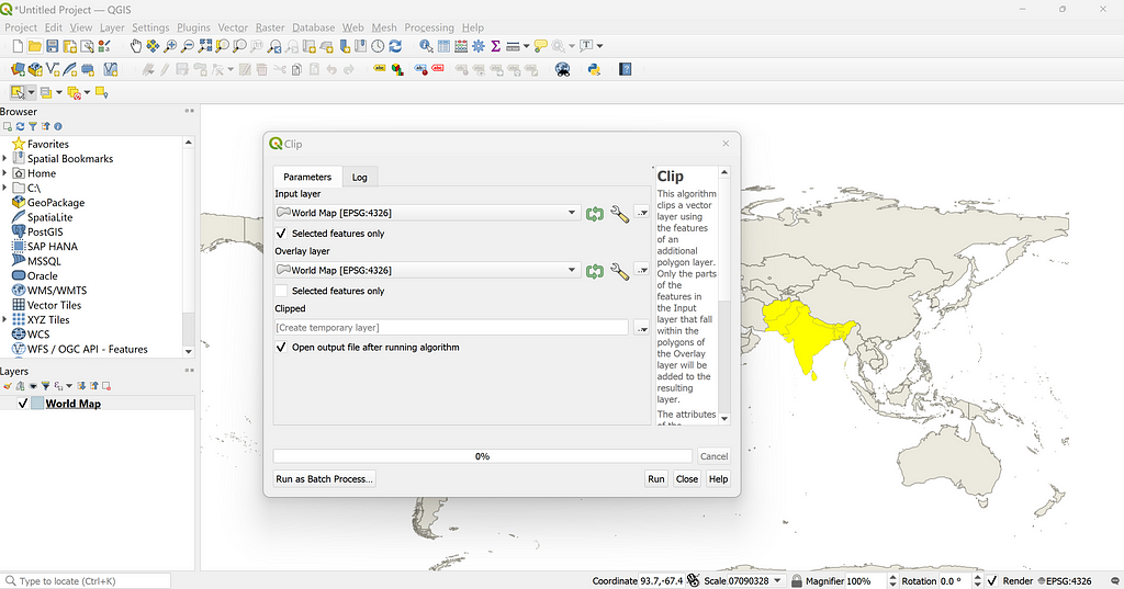
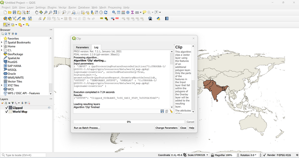
Polygon Tracing in Google Earth
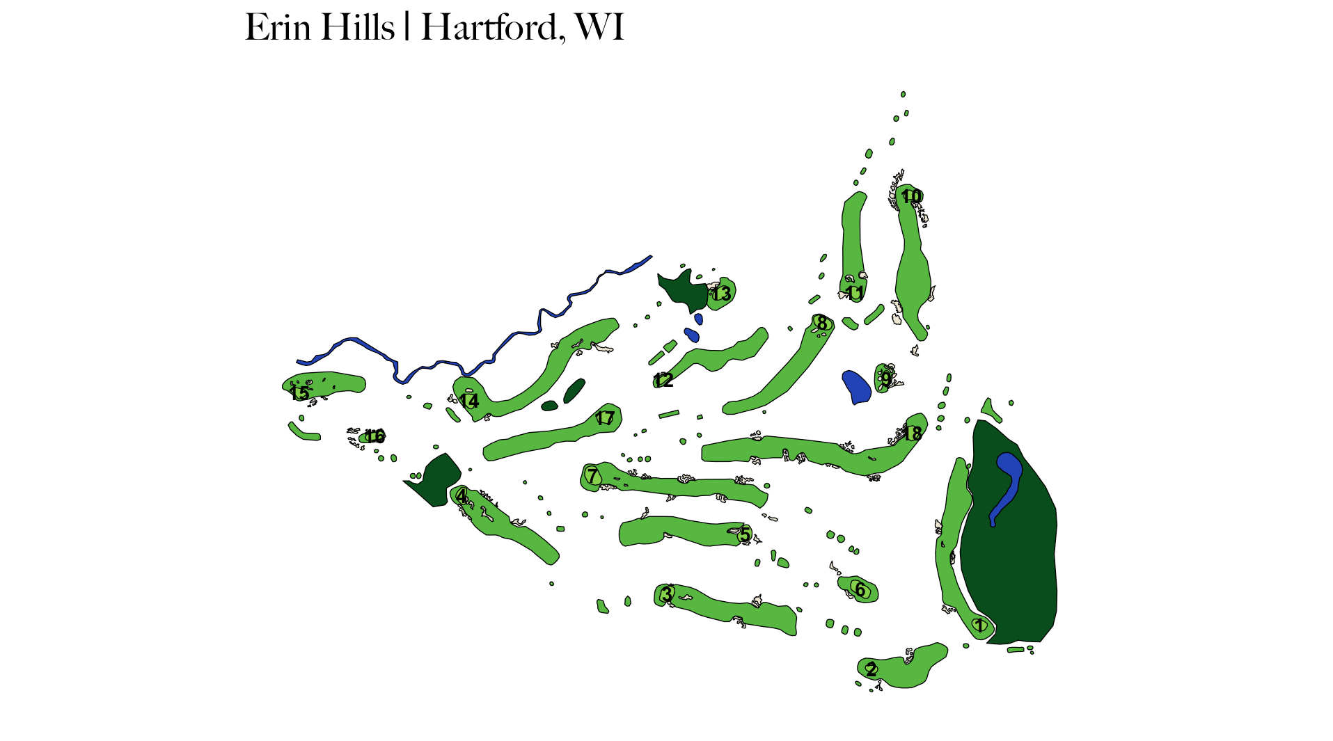
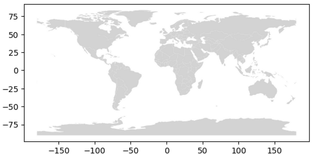
To begin, let’s head to Google Earth with a golf course in mind that we would like to plot. We will use Erin Hills in Wisconsin as a example. It is often helpful to either be familiar with the course layout or have a course map pulled up to more easily identify each hole via satellite imagery.
We will want to create a new project by clicking the blue “+ New” button in the top left corner. Next, we will use a Local KML file and click “Create”. Lastly, give the project a name, likely just the name of the course being mapped. The name of the project will be the name of the KML file we end up downloading upon completion.
Image from Google Earth, edited by the author
Now that our project folder is set up, we can start tracing. Disclaimer that Erin Hills has 138 bunkers, which I found out the hard way can be a bit tedious to trace… Anyway, let’s head to the first tee to start tracing.
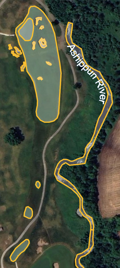
Once at the first tee, start by identifying the key elements of the hole. The first hole at Erin Hills has water and a hazard left of the fairway, a fairway dog-legging to the left, a few bunkers, etc. To begin tracing, click “Add path or polygon” which is the icon with a line and connected dots second from the left in the top toolbar. This will initialize a pencil of sorts that we can trace with.
Additional note: you can rotate your screen by simultaneously holding shift and pressing the left or right arrows.
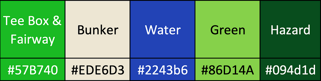
I typically start with the tee boxes, and work my way to the green. It is required that each traced polygon forms a closed shape, meaning you return to the original starting point. After finishing a polygon, save it to your project and give it a name. It is also important to name each polygon with a consistent naming convention, such as course_hole_element, which literally translates in this case to: erin_hills_hole_1_tee, or erin_hills_hole_5_fairway, etc. We will later use string matching in our R code to extract these key pieces of information from each polygon name. This will allow us to create a polygon element-to-color mapping, a.k.a. a way to tell ggplot2 how to color each polygon. So if “bunker” is the element, then we want to color it tan. If “water” is the element, it should be blue. It also allows us to extract the course name and hole numbers which open up additional plotting capabilities.
Below is Hole 15 at Erin Hills (my favorite from when I played there). The left image is the raw Google Earth image, the middle is after we have traced it, and the right image is after it has been rendered with ggplot2. I chose not to plot rough, trees, cart paths, etc.
(Left) Photo from Google Earth, (Middle) Photo from Google Earth, edited by author, (Right) Image by the author
Once we’ve finished mapping our hole or course, it is time to export all that hard work into a KML file. This can be done by clicking the three vertical dots on the left side of the screen where your project resides. This project works best with geoJSON data, which we can easily convert our KML file to in the next steps. Now we’re ready to head to R.
Plotting in R
The packages we will need to prepare us for plotting are: sf (for working with geospatial data), tidyverse (for data cleaning and plotting), stringr (for string matching), and geojsonsf (for converting from KML to geoJSON). Our first step is reading in the KML file, which can be done with the st_read() function from sf.
Great! Now we should have our golf course KML data in R. The data frame should have 2 columns: Name (project name, or course name in our case), and geometry (a list of all individual points comprising the polygons we traced). As briefly mentioned earlier, let’s convert our KML data to geoJSON and also extract the course name and hole numbers.
# convert from KML to geoJSON
geojson_df <- st_as_sf(kml_df, "POLYGON")

# extracting course name and hole number from polygon name
# assuming "course_hole_element" naming convention is used for polygons
geojson_df$course_name <- str_match(geojson_df$Name, “^(.+)_hole”)[,2]
geojson_df$hole_num <- gsub(“.*_hole_(\d+)_.*”, “\1”, geojson_df$Name)
To get our maps to point due north we need to project them in a way that preserves direction. We can do this with the st_transform() function.
# define a CRS for so map always points due north
crs <- "+proj=lcc +lat_1=33 +lat_2=45 +lat_0=39 +lon_0=-96 +x_0=0 +y_0=0 +datum=WGS84 +units=m +no_defs"

# transform data to CRS
geojson_df <- st_transform(geojson_df, crs)
We’re almost ready to plot, but first, we need to tell ggplot2 how each polygon should be colored. Below is the color palette my project is using, but feel free to customize as you wish.
Optional: in this step we can also calculate the centroids of our polygons with the st_centroid() function so we can overlay the hole number onto each green.
We’re officially ready to plot. We can use a combination of geom_sf(), geom_text(), and even geom_point() if we want to get fancy and plot shots on top of our map. I typically remove gridlines, axis labels, and the legend for a cleaner look.
If you followed along, had fun in doing so, or are intrigued, feel free to try mapping your favorite courses and create a Pull Request for the golfMapsR repository that I maintain: https://github.com/abodesy14/golfMapsR With some combined effort, we can create a nice little database of plottable golf courses around the world!
Choosing a college major was difficult for me. It felt like the first step to committing to a career and I wanted a little of everything. I liked math and programming, but I also wanted a job that allowed me to be creative, gave me a platform for communication, and was versatile enough to explore different industries. After some research, the data science program at the Halıcıoğlu Data Science Institute (HDSI) at UC San Diego seemed like a good fit. Despite my decision to pursue this path, I still had doubts and the assumptions I made at the start reflected this skepticism. However, as I work through my final quarters, I am glad (and surprised!) by how the realities of my experience have diverged from those expectations.
Expectation #1: Data science will be a lot of repetitive math and programming classes. The Reality: While math and programming are pillars, there is actually a lot of variety in classes.
Looking back, my classes have had much more variety than I expected. Programming and math classes are a majority but each course offers a different perspective on core topics while equipping us with a myriad of tools. There’s also significantly more diversity in the field, ranging from classes on statistical fairness definitions to bioinformatics. I also found niches I especially enjoyed in healthcare, data ethics, and privacy. This helped widen my perspectives on the roles and industries I could enter as a data scientist early on.
Expectation #2: I’d be working alone most of the time. The Reality: I work a lot with others and I am better for it.
I like working with people. Ideas are generated faster. I feel more creative and it’s just more fun! Nevertheless, I initially gave into the stereotype and pictured myself doing my data science homework hunched over a laptop for the better part of my day, so I was surprised by how much group work there was. Nearly all my programming and math classes encourage us to work with at least one other person. Meeting and working with people I didn’t know pushed me outside my comfort zone and refined my teamwork and communication skills. Even in professional settings when my work was independent, I found that working with other interns made me a better data scientist. Although we each had similar foundational skills, leaning on one another to utilize our different strengths and areas of focus allowed us to be better as a whole.
Expectation #3: Data science is the same as machine learning. The Reality: Machine learning is just a part of the data science project life cycle.
To be fair, I didn’t know much about data science or how machine learning (ML) was defined when I started my journey. Still, coming into the HDSI program, I thought data science was synonymous with ML. I imagined that most of my classes and work would be creating predictive models and delving into neural networks. Instead, the bulk of courses and work in data science focuses on data cleaning, data expiration, and visualization, with the ML analysis taking less time than you’d expect at the end… at least for now.
Expectation #4: My role could be automated. The Reality: Certain responsibilities can be automated but the creativity of data scientists as problem solvers can not.
This concern originated during my first natural language processing class where my professor showed how quickly GPT-3 could write code. It was daunting as an entry-level data scientist — how was I supposed to compete with models that could correctly write SQL queries faster than I could read them? However, this exercise was meant to illustrate that our roles as technologists weren’t just learning to use tools and understand the inherent processes that allow them to function. Large language models still can’t do your homework correctly, but eventually (and inevitably) they will improve, and when they do, I’m optimistic that they’ll be more of an aid rather than a detriment to data scientists. Unlike data scientists, LLMs aren’t problem solvers. They can’t generate original ideas, use creativity to navigate ambiguous problems, or effectively communicate with different audiences. This may change in the future but through my education and professional experiences, I am confident that I can still make a positive impact in the field.
The Takeaway
As a part of my data science journey, I’ve learned to embrace the unexpectedness that comes with reality. I learned that the breadth and depth of data science were ideal for doing a bit of everything: to research, to program, to analyze, and to tell stories. With that, I’m confident in my decision to pursue data science and excited to see what the next phase of my career brings.
Applying machine learning methodology to prompt building
Drawn by the author
LLMs are grounded in data science, but our approach to prompt engineering might strike us as unscientific:
Manual prompt engineering which does not generalize well: LLMs are highly sensitive to how they are prompted for each task, so we need to handcraft long strings of instructions and demonstrations. This requires not only time-consuming prompt writing process, but the given string prompt might not generalize to different pipelines or across different LMs, data domains, or even inputs. To deal with a new problem we often need to handcraft a new prompt.
Lack framework to conduct testing: Instead of the usual train-test regime in typical data science applications to pick the model which maximizes a certain metric like AUC, with LLMs we arrive at the best prompt via trial and error, often without an objective metric to say how well our model is performing. Thus no matter how we try to improve the prompt, we can’t confidently say how reliable our application is.
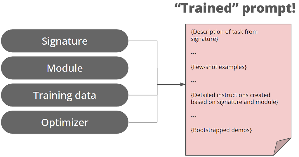
To address these issues, Stanford NLP has published a paper introducing a new approach with prompt writing: instead of manipulating free-form strings, we generate prompts via modularized programming. The associated library, called DSPy, can be found here.
This article aims to show how this “prompt programming” is done, to go deeper in explaining what’s happening behind the optimization process. The code can also be found here.
(Speaking of which, you might also find coaxing LLMs to output properly formatted JSON very unscientific too, I have also written an article about how to address this with Function Calling. Check it out !)
We will spend some time to go over the environment preparation. Afterwards, this article is divided into 3 sections:
Basic concept of DSPy: Signature and Module Basic building blocks in DSPy for describing your task, and the prompt technique used
Optimizer: Train our prompt as with machine learning How DSPy optimizes your prompt with bootstrapping
Full fledged example: Prompt comparison with LLM Applying the rigour of traditional machine learning for prompt testing and selection
We are now ready to start!
Preparation
Head over to Github to clone my code. The contents in my article can be found in the dspy_tutorial Notebook.
Please also create and activate a virtual environment, then pip install -r requirements.txt to install the required packages. If you are on Windows, please also install Windows C++ build tools which are required for the phoneix library with which we will observe how DSPy works
My code uses OpenRouter, which allow us to access OpenAI API in blocked regions. Please set up your OPENROUTER_API_KEY as environment variable, and execute the code under the “Preparation” block. Alternatively, you can use dspy.OpenAI class directly and define Open AI API key if it works for you
Basic concept of DSPy: Signature and Module
They are the building blocks of prompt programming in DSPy. Let’s dive in to see what they are about!
Signatures: Specification of input/output
A signature is the most fundamental building block in DSPy’s prompt programming, which is a declarative specification of input/output behavior of a DSPy module. Signatures allow you to tell the LM what it needs to do, rather than specify how we should ask the LM to do it.
Say we want to obtain the sentiment of a sentence, traditionally we might write such prompt:
Given a sentence {the_sentence_itself}, deduce its sentiment.
But in DSPy, we can achieve the same by defining a signature as below. At its most basic form, a signature is as simple as a single string separating the inputs and output with a ->
Note: Code in this section contains those referred from DSPy’s documentation of Signatures
# Run sentence = "it's a charming and often affecting journey." classify(sentence=sentence).sentiment
--- Output ---
"I'm sorry, but I am unable to determine the sentiment of the sentence without additional context or information. If you provide me with more details or specific criteria for determining sentiment, I would be happy to assist you further."
The prediction is not a good one, but for instructional purpose let’s inspect what was the issued prompt.
# This is how we inpect the last issued prompt to the LM
lm.inspect_history(n=1)
--- Output ---
Given the fields `sentence`, produce the fields `sentiment`.

---

Follow the following format.

Sentence: ${sentence}
Sentiment: ${sentiment}

---

Sentence: it's a charming and often affecting journey.
Sentiment: I'm sorry, but I am unable to determine the sentiment of the sentence without additional context or information. If you provide me with more details or specific criteria for determining sentiment, I would be happy to assist you further.
We can see the above prompt is assembled from the sentence -> sentiment signature. But how did DSPy came up with the Given the fields… in the prompt?
Inspecting the dspy.Predict() class, we see when we pass to it our signature, the signature will be parsed as the signature attribute of the class, and subsequently assembled as a prompt. The instructions is a default one hardcoded in the DSPy library.
# Check the variables of the `classify` object,
# which was created by passing the signature to `dspy.Predict()` class
vars(classify)
What if we want to provide a more detailed description of our objective to the LLM, beyond the basic sentence -> sentiment signature? To do so we need to provide a more verbose signature in form of Class-based DSPy Signatures.
Notice we provide no explicit instruction as to how the LLM should obtain the sentiment. We are just describing the task at hand, and also the expected output.
# Define signature in Class-based form class Emotion(dspy.Signature): # Describe the task """Classify emotions in a sentence."""
sentence = dspy.InputField() # Adding description to the output field sentiment = dspy.OutputField(desc="Possible choices: sadness, joy, love, anger, fear, surprise.")
--- Output ---
Sentence: It's a charming and often affecting journey.
Sentiment: joy
It is now outputting a much better prediction! Again we see the descriptions we made when defining the class-based DSPy signatures are assembled into a prompt.
Sentence: it's a charming and often affecting journey. Sentiment: Sentence: It's a charming and often affecting journey. Sentiment: joy
This might do for simple tasks, but advanced applications might require sophisticated prompting techniques like Chain of Thought or ReAct. In DSPy these are implemented as Modules
Modules: Abstracting prompting techniques
We may be used to apply “prompting techniques” by hardcoding phrases like let’s think step by step in our prompt . In DSPy these prompting techniques are abstracted as Modules. Let’s see below for an example of applying our class-based signature to the dspy.ChainOfThought module
# Apply the class-based signature to Chain of Thought
classify_cot = dspy.ChainOfThought(Emotion)

# Run
classify_cot(sentence=sentence).sentiment

# Inspect prompt
lm.inspect_history(n=1)
--- Output ---
Classify emotions in a sentence.

---

Follow the following format.

Sentence: ${sentence}
Reasoning: Let's think step by step in order to ${produce the sentiment}. We ...
Sentiment: Possible choices: sadness, joy, love, anger, fear, surprise.

---

Sentence: it's a charming and often affecting journey.
Reasoning: Let's think step by step in order to Sentence: It's a charming and often affecting journey.
Reasoning: Let's think step by step in order to determine the sentiment. The use of the words "charming" and "affecting" suggests positive emotions associated with enjoyment and emotional impact. We can infer that the overall tone is positive and heartwarming, evoking feelings of joy and possibly love.
Sentiment: Joy, love
Notice how the “Reasoning: Let’s think step by step…” phrase is added to our prompt, and the quality of our prediction is even better now.
According to DSPy’s documentation, as of time of writing DSPy provides the following prompting techniques in form of Modules. Notice the dspy.Predict we used in the initial example is also a Module, representing no prompting technique!
dspy.Predict: Basic predictor. Does not modify the signature. Handles the key forms of learning (i.e., storing the instructions and demonstrations and updates to the LM).
dspy.ChainOfThought: Teaches the LM to think step-by-step before committing to the signature’s response.
dspy.ProgramOfThought: Teaches the LM to output code, whose execution results will dictate the response.
dspy.ReAct: An agent that can use tools to implement the given signature.
dspy.MultiChainComparison: Can compare multiple outputs from ChainOfThought to produce a final prediction.
It also have some function-style modules:
6. dspy.majority: Can do basic voting to return the most popular response from a set of predictions.
Then we define the RAG class inherited from dspy.Module. It needs two methods:
The __init__ method will simply declare the sub-modules it needs: dspy.Retrieve and dspy.ChainOfThought. The latter is defined to implement our context, question -> answer signature.
The forward method will describe the control flow of answering the question using the modules we have.
# Define a class-based signature class GenerateAnswer(dspy.Signature): """Answer questions with short factoid answers."""
context = dspy.InputField(desc="may contain relevant facts") question = dspy.InputField() answer = dspy.OutputField(desc="often between 1 and 5 words")
# Chain different modules together to retrieve information from Wikipedia Abstracts 2017, then pass it as context for Chain of Thought to generate an answer class RAG(dspy.Module): def __init__(self, num_passages=3): super().__init__() self.retrieve = dspy.Retrieve(k=num_passages) self.generate_answer = dspy.ChainOfThought(GenerateAnswer)
# Define a question and pass it into the RAG class my_question = "When was the first FIFA World Cup held?" rag(question=my_question).answer
--- Output ---
'1930'
Inspecting the prompt, we see that 3 passages retrieved from Wikipedia Abstracts 2017 is interpersed as context for Chain of Thought generation
Answer questions with short factoid answers.

---

Follow the following format.

Context: may contain relevant facts

Question: ${question}

Reasoning: Let's think step by step in order to ${produce the answer}. We ...

Answer: often between 1 and 5 words

---

Context:
[1] «History of the FIFA World Cup | The FIFA World Cup was first held in 1930, when FIFA president Jules Rimet decided to stage an international football tournament. The inaugural edition, held in 1930, was contested as a final tournament of only thirteen teams invited by the organization. Since then, the World Cup has experienced successive expansions and format remodeling to its current 32-team final tournament preceded by a two-year qualifying process, involving over 200 teams from around the world.»
[2] «1950 FIFA World Cup | The 1950 FIFA World Cup, held in Brazil from 24 June to 16 July 1950, was the fourth FIFA World Cup. It was the first World Cup since 1938, the planned 1942 and 1946 competitions having been cancelled owing to World War II. It was won by Uruguay, who had won the inaugural competition in 1930, clinching the cup by beating the hosts Brazil 2–1 in the deciding match of the four-team final group (this was the only tournament not decided by a one-match final). It was also the first tournament where the trophy was referred to as the Jules Rimet Cup, to mark the 25th anniversary of Jules Rimet's presidency of FIFA.»
[3] «1970 FIFA World Cup | The 1970 FIFA World Cup was the ninth FIFA World Cup, the quadrennial international football championship for men's national teams. Held from 31 May to 21 June in Mexico, it was the first World Cup tournament staged in North America, and the first held outside Europe and South America. Teams representing 75 nations from all six populated continents entered the competition, and its qualification rounds began in May 1968. Fourteen teams qualified from this process to join host nation Mexico and defending champions England in the sixteen-team final tournament. El Salvador, Israel, and Morocco made their first appearances at the final stage, and Peru their first since 1930.»

Question: When was the first FIFA World Cup held?

Reasoning: Let's think step by step in order to Answer: 1930

Answer: 1930
The above examples might not seem much. At its most basic application the DSPy seemed only doing nothing that can’t be done with f-string, but it actually present a paradigm shift for prompt writing, as this brings modularity to prompt composition!
First we describe our objective with Signature, then we apply different prompting techniques with Modules. To test different prompt techniques for a given problem, we can simply switch the modules used and compare their results, rather than hardcoding the “let’s think step by step…” (for Chain of Thought) or “you will interleave Thought, Action, and Observation steps” (for ReAct) phrases. The benefit of modularity will be demonstrated later in this article with a full-fledged example.
The power of DSPy is not only limited to modularity, it can also optimize our prompt based on training samples, and test it systematically. We will be exploring this in the next section!
Optimizer: Train our prompt as with machine learning
In this section we try to optimize our prompt for a RAG application with DSPy.
Taking Chain of Thought as an example, beyond just adding the “let’s think step by step” phrase, we can boost its performance with a few tweaks:
Adding suitable examples (aka few-shot learning).
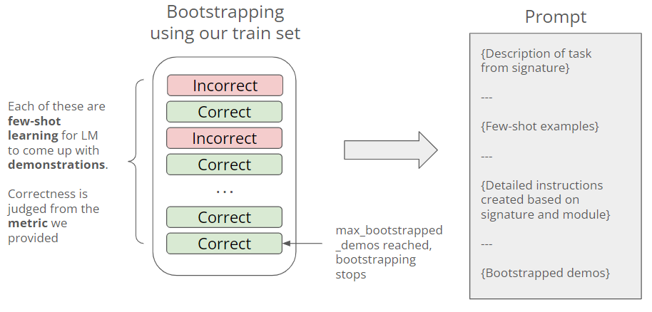
Furthermore, we can bootstrap demonstrations of reasoning to teach the LMs to apply proper reasoning to deal with the task at hand.
Doing this manually would be highly time-consuming and can’t generalize to different problems, but with DSPy this can be done automatically. Let’s dive in!
Preparation
#1: Loading test data: Like machine learning, to train our prompt we need to prepare our training and test datasets. Initially this cell will take around 20 minutes to run.
from dspy.datasets.hotpotqa import HotPotQA

# For demonstration purpose we will use a small subset of the HotPotQA dataset, 20 for training and testing each
dataset = HotPotQA(train_seed=1, train_size=20, eval_seed=2023, dev_size=20, test_size=0)
trainset = [x.with_inputs('question') for x in dataset.train]
testset = [x.with_inputs('question') for x in dataset.dev]

len(trainset), len(testset)
Inspecting our dataset, which is basically a set of question-and-answer pairs
Example({'question': 'At My Window was released by which American singer-songwriter?', 'answer': 'John Townes Van Zandt'}) (input_keys={'question'})
#2 Set up Phoenix for observability: To facilitate understanding of the optimization process, we launch Phoenix to observe our DSPy application, which is a great tool for LLM observability in general! I will skip pasting the code here, but you can execute it in the notebook.
Note: If you are on Windows, please also install Windows C++ Build Tools here, which is necessary for Phoenix
Prompt Optimization
Then we are ready to see what this opimitzation is about! To “train” our prompt, we need 3 things:
A training set. We’ll just use our 20 question–answer examples from trainset.
A metric for validation. Here we use the native dspy.evaluate.answer_exact_match which checks if the predicted answer exactly matches the right answer (questionable but suffice for demonstration). For real-life applications you can define your own evaluation criteria
A specific Optimizer (formerly teleprompter). The DSPy library includes a number of optimization strategies and you can check them out here. For our example we use BootstrapFewShot. Instead of describing it here with lengthy description, I will demonstrate it with code subsequently
Now we train our prompt.
from dspy.teleprompt import BootstrapFewShot
# Simple optimizer example. I am explicitly stating the default values for max_bootstrapped_demos and max_labeled_demos for demonstration purposes optimizer = BootstrapFewShot(metric=dspy.evaluate.answer_exact_match, max_bootstrapped_demos=4)
--- Successful execution should show this output ---
Bootstrapped 4 full traces after n examples in round 0
Before using the compiled_rag to answer a question, let’s see what went behind the scene during the training process (aka compile). We launch the Phoenix console by visiting http://localhost:6006/ in browser
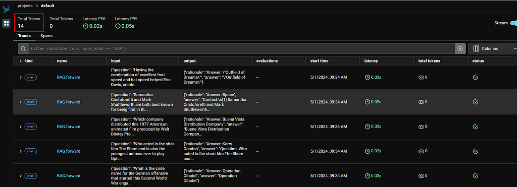
14 calls during “compile”
In my run I have made 14 calls using the RAG class, in each of those calls we post a question to LM to obtain a prediction.
Refer to the result summary table in my notebook, 4 correct answers are made from these 14 samples, thus reaching our max_bootstrapped_demos parameter and stopping the calls.
But what are the prompts DSPy issued to obtain the bootstrapped demos? Here’s the prompt for question #14. We can see as DSPy tries to generate one bootstrapped demo, it would randomly add samples from our trainset for few-short learning.
Answer questions with short factoid answers.

---

{Pairs of question-and-answer as samples}

---

Follow the following format.

Context: may contain relevant facts

Question: ${question}

Reasoning: Let's think step by step in order to ${produce the answer}. We ...

Answer: often between 1 and 5 words

---

Context:
[1] «Eric Davis (baseball) | Eric Keith Davis (born May 29, 1962) is a former center fielder for several Major League Baseball teams. Davis was 21 years old when he broke into the big leagues on May 19, 1984 with the Cincinnati Reds, the team for which he is most remembered. Blessed with a rare combination of excellent foot speed and bat speed, Davis became the first major league player to hit at least 30 home runs and steal at least 50 bases in the same season in 1987.»
[2] «Willie Davis (baseball) | William Henry Davis, Jr. (April 15, 1940 – March 9, 2010) was a center fielder in Major League Baseball who played most of his career for the Los Angeles Dodgers. At the end of his career he ranked seventh in major league history in putouts (5449) and total chances (5719) in the outfield, and third in games in center field (2237). He was ninth in National League history in total outfield games (2274), and won Gold Glove Awards from 1971 to 1973. He had 13 seasons of 20 or more stolen bases, led the NL in triples twice, and retired with the fourth most triples (138) by any major leaguer since 1945. He holds Los Angeles club records (1958–present) for career hits (2091), runs (1004), triples (110), at bats (7495), total bases (3094) and extra base hits (585). His 31-game hitting streak in 1969 remains the longest by a Dodger. At one point during the streak, when the team was playing at home, the big message board at Dodger Stadium quoted a message from a telegram sent to Davis and the team from Zack Wheat, the team's former record holder, at his home in Missouri.»
[3] «1992 Los Angeles Dodgers season | The 1992 Los Angeles Dodgers season was a poor one for the team as it finished last in the Western Division of the National League with a record of 63 wins and 99 losses. Despite boasting what was nicknamed the "Outfield of Dreams", being manned by Eric Davis, Brett Butler, and Darryl Strawberry, injuries to key players and slumps from others contributed to the franchise's worst season since moving to Los Angeles. Additionally, the Dodgers cancelled four home games during the season due to the L.A. Riots. Despite the poor finish, the Dodgers had some hope for the future as first baseman Eric Karros won the National League Rookie of the Year Award, the first of five consecutive Dodger players to do so. The 1992 season also saw the Dodgers drop television station KTTV Ch.11 as their chief broadcaster of Dodger baseball, ending a 34 year-35 consecutive season association with that station. Additionally, it was the first time the Dodgers lost 90 games in a season since 1944.»

Question: Having the combination of excellent foot speed and bat speed helped Eric Davis, create what kind of outfield for the Los Angeles Dodgers?

Reasoning: Let's think step by step in order to Answer: "Outfield of Dreams"

Answer: "Outfield of Dreams"
Time to put the compiled_rag to test! Here we raise a question which was answered wrongly in our summary table, and see if we can get the right answer this time.
compiled_rag(question="Which of these publications was most recently published, Who Put the Bomp or Self?")
Again let’s inspect the prompt issued. Notice how the compiled prompt is different from the ones that were used during bootstrapping. Apart from the few-shot examples, bootstrapped Context-Question-Reasoning-Answer demonstrations from correct predictions are added to the prompt, improving the LM’s capability.
Answer questions with short factoid answers.

---

{Pairs of question-and-answer as samples}

---

Follow the following format.

Context: may contain relevant facts

Question: ${question}

Reasoning: Let's think step by step in order to ${produce the answer}. We ...

Answer: often between 1 and 5 words

---

{4 sets of Context-Question-Reasoning-Answer demonstrations}

---

Context:
[1] «Who Put the Bomp | Who Put The Bomp was a rock music fanzine edited and published by Greg Shaw from 1970 to 1979. Its name came from the hit 1961 doo-wop song by Barry Mann, "Who Put the Bomp". Later, the name was shortened to "Bomp!"»
[2] «Bompiani | Bompiani is an Italian publishing house based in Milan, Italy. It was founded in 1929 by Valentino Bompiani.»
[3] «What Color is Your Parachute? | What Color is Your Parachute? by Richard Nelson Bolles is a book for job-seekers that has been in print since 1970 and has been revised every year since 1975, sometimes substantially. Bolles initially self-published the book (December 1, 1970), but it has been commercially published since November 1972 by Ten Speed Press in Berkeley, California. As of September 28, 2010, the book is available in 22 languages, it is used in 26 countries around the world, and over ten million copies have been sold worldwide. It is one of the most highly regarded career advice books in print. In the latest edition of the book, the author writes about how to adapt one's job search to the Web 2.0 age.»

Question: Which of these publications was most recently published, Who Put the Bomp or Self?

Reasoning: Let's think step by step in order to Answer: Self

Answer: Self
So the below is basically went behind the scene with BootstrapFewShot during compilation:
Bootstrapping demonstrations to enhance the prompt
The above example still falls short of what we typically do with machine learning: Even boostrapping maybe useful, we are not yet proving it to improve the quality of the responses.
Ideally, like in traditional machine learning we should define a couple of candidate models, see how they perform against the test set, and select the one achieving the highest performance score. This is what we will do next!
Full fledged example: Prompt comparison with LLM
The aim of this example
In this section, we want to evaluate what is the “best prompt” (expressed in terms of module and optimizer combination) to perform a RAG against the HotpotQA dataset (distributed under a CC BY-SA 4.0 License), given the LM we use (GPT 3.5 Turbo).
The Modules under evaluation are:
Vanilla: Single-hop RAG to answer a question based on the retrieved context, without key phrases like “let’s think step by step”
COT: Single-hop RAG with Chain of Thought
ReAct: Single-hop RAG with ReAct prompting
BasicMultiHop: 2-hop RAG with Chain of Thought
And the Optimizer candidates are:
None: No additional instructions apart from the signature
Bootstrap few-shot: As we demonstrated, self-generate complete demonstrations for every stage of our module. Will simply use the generated demonstrations (if they pass the metric) without any further optimization. For Vanilla it is just equal to “Labeled few-shot”
As for evaluation metric, we again use exact match as criteria (dspy.evaluate.metrics.answer_exact_match) against the test set.
Then I defined a helper class to facilitate the evaluation. The code is a tad bit long so I am not pasting it here, but it could be found in my notebook. What it does is to apply each the optimizers against the modules, compile the prompt, then perform evaluation against the test set.
We are now ready to start the evaluation, it would take around 20 minutes to complete
# Compile the models
ms = ModelSelection(modules=modules, optimizers=optimizers, metric=metric, trainset=trainset)

# Evaluate them
ms.evaluate(testset=testset)
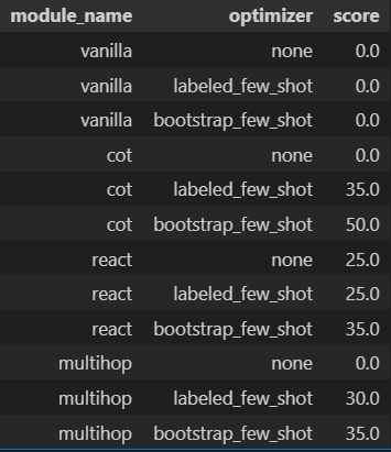
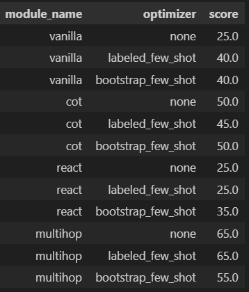
Here’s the evaluation result. We can see the COT module with BootstrapFewShot optimizer has the best performance. The scores represent the percentage of correct answers (judged by exact match) made for the test set.
But before we conclude the exercise, it might be useful to inspect the result more deeply: Multihop with BootstrapFewShot, which supposedly equips with more relevant context than COT with BootstrapFewShot, has a worse performance. It is strange!
Debug and fine-tune our prompt
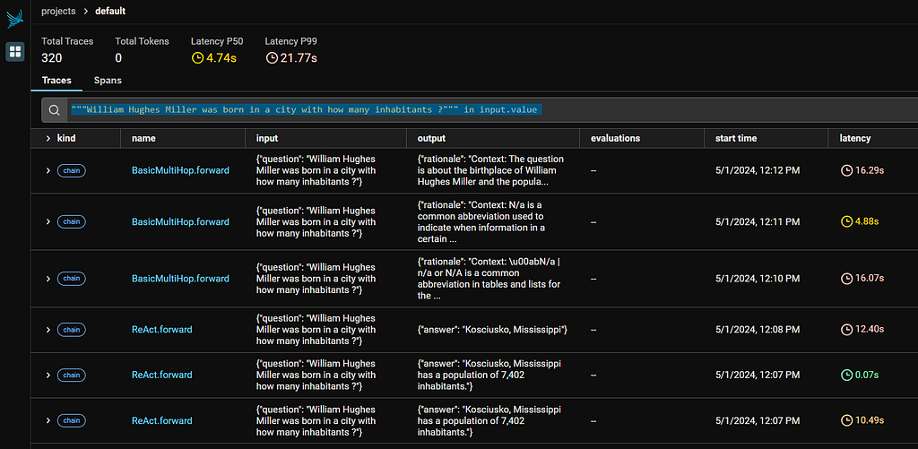
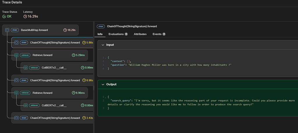
Now head to the Phoenix Console to see what’s going on. We pick a random question William Hughes Miller was born in a city with how many inhabitants ?, and inspect how did COT, ReAct, BasicMultiHop with BoostrapFewShot optimizer came up with their answer. You can type this in the search bar for filter: “””William Hughes Miller was born in a city with how many inhabitants ?””” in input.value
The calls follow sequential order, so for each of the module we can pick the BootstrapFewShot variant by picking the 3rd call
These are the answers provided by the 3 models during my run:
Multihop with BootstrapFewShot: The answer will vary based on the specific city of William Hughes Miller’s birthplace.
ReAct with BootstrapFewShot: Kosciusko, Mississippi
COT with BootstrapFewShot: The city of Kosciusko, Mississippi, has a population of approximately 7,402 inhabitants.
The correct answer is 7,402 at the 2010 census. Both ReAct with BootstrapFewShot and COT with BootstrapFewShot provided relevant answers, but Multihop with BootstrapFewShot simply failed to provide one.
Checking the execution trace in Phoenix for Multihop with BootstrapFewShot, looks like the LM fails to understand what is expected for the search_query specified in the signature.
The LM can’t come up with the search_query during the 1st hop
So we revise the signature, and re-run the evaluation with the code below
# Define a class-based signature
class GenerateAnswer(dspy.Signature):
    """Answer questions with short factoid answers."""

    context = dspy.InputField(desc="may contain relevant facts")
    question = dspy.InputField()
    answer = dspy.OutputField(desc="often between 1 and 5 words")

class BasicQA(dspy.Signature):
    """Answer questions with short factoid answers."""

    question = dspy.InputField()
    answer = dspy.OutputField(desc="often between 1 and 5 words")

class FollowupQuery(dspy.Signature):
    """Generate a query which is conducive to answering the question"""

    context = dspy.InputField(desc="may contain relevant facts")
    question = dspy.InputField()
    search_query = dspy.OutputField(desc="Judge if the context is adequate to answer the question, if not adequate or if it is blank, generate a search query that would help you answer the question.")
# Revise the modules with the class-based signatures. You can find the relevant code in my notebook # To keep the article concise I am not pasting it here.
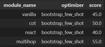
# Then run the below command to re-compile and evaluate ms_revised = ModelSelection(modules=modules_revised, optimizers=optimizers, metric=metric, trainset=trainset) ms_revised.evaluate(testset=testset) ms_revised.evaluation_matrix
Performance improved after updating the signatures
We now see the score improved across all models, and Multihop with LabeledFewShot and Multihop with no examples now have the best performance! This indicates despite DSPy tries to optimize the prompt, there is still some prompt engineering involved by articulating your objective in signature.
The best model now produce an exact match for our question!
# The correct answer is 7,402
question = """`William Hughes Miller was born in a city with how many inhabitants ?"""
ms_revised.question_for_model('multihop','labeled_few_shot',question)
Since the best prompt is Multihop with LabeledFewShot, the prompt does not contain bootstrapped Context-Question-Reasoning-Answer demonstrations. So bootstrapping may not surely lead to better performance, we need to prove which one is the best prompt scientifically.
Answer questions with short factoid answers.

---

{Pairs of question-and-answer as samples}

---

Follow the following format.

Context: may contain relevant facts

Question: ${question}

Reasoning: Let's think step by step in order to ${produce the answer}. We ...

Answer: often between 1 and 5 words

---

Context:
[1] «William Hughes Miller | William Hughes Miller (born March 16, 1941, Kosciusko, Mississippi) is a professor at the University of California, Berkeley and a leading researcher in the field of theoretical chemistry.»
[2] «William Herbert Miller, Jr. | William Hubert Miller, Jr. (September 1932 – November 4, 1988), of New York City, was an aerophilatelist who published philatelic literature on the subject.»
[3] «William Green Miller | William Green Miller (born August 15, 1931 in New York City, New York), served as the United States Ambassador to Ukraine under Bill Clinton, from 1993 to 1998.»
[4] «Kosciusko, Mississippi | Kosciusko is a city in Attala County, Mississippi, United States. The population was 7,402 at the 2010 census. It is the county seat of Attala County.»
[5] «Attala County, Mississippi | Attala County is a county located in the U.S. state of Mississippi. As of the 2010 census, the population was 19,564. Its county seat is Kosciusko. Attala County is named for Atala, a fictional Native American heroine from an early-19th-century novel of the same name by François-René de Chateaubriand.»
[6] «Kosciusko Island | Kosciusko Island is an island in the Alexander Archipelago of southeastern Alaska, United States. It lies near the northwest corner of Prince of Wales Island, just across the El Capitan Passage from the larger island. The island is near Mount Francis, Holbrook Mountain, and Tokeen Peak. Kosciusko Island has a land area of 171.585 sq mi (444.403 km²), making it the 38th largest island in the United States. It had a population of 52 persons as of the 2000 census, mostly in Edna Bay, its largest community.»

Question: `William Hughes Miller was born in a city with how many inhabitants ?

Reasoning: Let's think step by step in order to Answer: 7,402

Answer: 7,402
It does not mean Multihop with BootstrapFewShot has a worse performance in general however. Only that for our task, if we use GPT 3.5 Turbo to bootstrap demonstration (which might be of questionable quality) and output prediction, then we might better do without the bootstrapping, and keep only the few-shot examples.
This lead to the question: Is it possible to use a more powerful LM, say GPT 4 Turbo (aka teacher) to generate demonstrations, while keeping cheaper models like GPT 3.5 Turbo (aka student) for prediction?
“Teacher” to power-up bootstrapping capability
The answer is YES as the following cell demonstrates, we will use GPT 4 Turbo as teacher.
# Define the GPT-4 Turbo model
gpt4_turbo = dspy.Databricks(api_key=OPENROUTER_API_KEY,
  api_base="https://openrouter.ai/api/v1",
  model="openai/gpt-4-turbo")

# Define new Optimizer which uses GPT-4 Turbo as a teacher
optimizers_gpt4_teacher = {
    'bootstrap_few_shot': BootstrapFewShot(metric=metric, max_errors=20, teacher_settings=dict(lm=gpt4_turbo)),
}

# Compile the models and evaluate them as before
ms_gpt4_teacher = ModelSelection(modules=modules_revised, optimizers=optimizers_gpt4_teacher, metric=metric, trainset=trainset)
ms_gpt4_teacher.evaluate(testset=testset)
ms_gpt4_teacher.evaluation_matrix
Result using GPT-4 as teacher
Using GPT-4 Turbo as teacher does not significantly boost our models’ performance however. Still it is worthwhile to see its effect to our prompt. Below is the prompt generated just using GPT 3.5
Answer questions with short factoid answers.

---

{Pairs of question-and-answer as samples}

---

Follow the following format.

Context: may contain relevant facts

Question: ${question}

Reasoning: Let's think step by step in order to ${produce the answer}. We ...

Answer: often between 1 and 5 words

---

Context:
[1] «Candace Kita | Kita's first role was as a news anchor in the 1991 movie "Stealth Hunters". Kita's first recurring television role was in Fox's "Masked Rider", from 1995 to 1996. She appeared as a series regular lead in all 40 episodes. Kita also portrayed a frantic stewardess in a music video directed by Mark Pellington for the British group, Catherine Wheel, titled, "Waydown" in 1995. In 1996, Kita also appeared in the film "Barb Wire" (1996) and guest starred on "The Wayans Bros.". She also guest starred in "Miriam Teitelbaum: Homicide" with "Saturday Night Live" alumni Nora Dunn, "Wall To Wall Records" with Jordan Bridges, "Even Stevens", "Felicity" with Keri Russell, "V.I.P." with Pamela Anderson, "Girlfriends", "The Sweet Spot" with Bill Murray, and "Movies at Our House". She also had recurring roles on the FX spoof, "Son of the Beach" from 2001 to 2002, ABC-Family's "Dance Fever" and Oxygen Network's "Running with Scissors". Kita also appeared in the films "Little Heroes" (2002) and "Rennie's Landing" (2001).»
[2] «Jilly Kitzinger | Jilly Kitzinger is a fictional character in the science fiction series "Torchwood", portrayed by American actress Lauren Ambrose. The character was promoted as one of five new main characters to join "Torchwood" in its fourth series, "" (2011), as part of a new co-production between "Torchwood"' s British network, BBC One, and its American financiers on US premium television network Starz. Ambrose appears in seven of the ten episodes, and is credited as a "special guest star" throughout. Whilst reaction to the serial was mixed, Ambrose' portrayal was often singled out by critics for particular praise and in 2012 she received a Saturn Award nomination for Best Supporting Actress on Television.»
[3] «Candace Brown | Candace June Brown (born June 15, 1980) is an American actress and comedian best known for her work on shows such as "Grey's Anatomy", "Desperate Housewives", "Head Case", The "Wizards Of Waverly Place". In 2011, she joined the guest cast for "Torchwood"' s fourth series' "", airing on BBC One in the United Kingdom and premium television network Starz.»
[4] «Candace Kita | Kita's first role was as a news anchor in the 1991 movie "Stealth Hunters". Kita's first recurring television role was in Fox's "Masked Rider", from 1995 to 1996. She appeared as a series regular lead in all 40 episodes. Kita also portrayed a frantic stewardess in a music video directed by Mark Pellington for the British group, Catherine Wheel, titled, "Waydown" in 1995. In 1996, Kita also appeared in the film "Barb Wire" (1996) and guest starred on "The Wayans Bros.". She also guest starred in "Miriam Teitelbaum: Homicide" with "Saturday Night Live" alumni Nora Dunn, "Wall To Wall Records" with Jordan Bridges, "Even Stevens", "Felicity" with Keri Russell, "V.I.P." with Pamela Anderson, "Girlfriends", "The Sweet Spot" with Bill Murray, and "Movies at Our House". She also had recurring roles on the FX spoof, "Son of the Beach" from 2001 to 2002, ABC-Family's "Dance Fever" and Oxygen Network's "Running with Scissors". Kita also appeared in the films "Little Heroes" (2002) and "Rennie's Landing" (2001).»
[5] «Kiti Manver | María Isabel Ana Mantecón Vernalte (born 11 May 1953) better known as Kiti Mánver is a Spanish actress. She has appeared in more than 100 films and television shows since 1970. She starred in the 1973 film "Habla, mudita", which was entered into the 23rd Berlin International Film Festival.»
[6] «Amy Steel | Amy Steel (born Alice Amy Steel; May 3, 1960) is an American film and television actress. She is best known for her roles as Ginny Field in "Friday the 13th Part 2" (1981) and Kit Graham in "April Fool's Day" (1986). She has starred in films such as "Exposed" (1983), "Walk Like a Man" (1987), "What Ever Happened to Baby Jane? " (1991), and "Tales of Poe" (2014). Steel has had numerous guest appearances on several television series, such as "Family Ties" (1983), "The A-Team" (1983), "Quantum Leap" (1990), and "China Beach" (1991), as well as a starring role in "The Powers of Matthew Star" (1982–83).»

Question: which American actor was Candace Kita guest starred with

Reasoning: Let's think step by step in order to Answer: Bill Murray

Answer: Bill Murray

---

Context:
[1] «Monthly Magazine | The Monthly Magazine (1796–1843) of London began publication in February 1796. Richard Phillips was the publisher and a contributor on political issues. The editor for the first ten years was the literary jack-of-all-trades, Dr John Aikin. Other contributors included William Blake, Samuel Taylor Coleridge, George Dyer, Henry Neele and Charles Lamb. The magazine also published the earliest fiction of Charles Dickens, the first of what would become "Sketches by Boz".»
[2] «Bodega Magazine | Bodega Magazine is an online literary magazine that releases new issues on the first Monday of every month, featuring stories, poems, essays and interviews from a mix of emerging and established writers. It was founded in early spring of 2012 by creative writing MFA graduates from New York University who had previously worked together on the "Washington Square Review", and continues to be based out of Manhattan and Brooklyn. The inaugural issue was published on September 4, 2012.»
[3] «Who Put the Bomp | Who Put The Bomp was a rock music fanzine edited and published by Greg Shaw from 1970 to 1979. Its name came from the hit 1961 doo-wop song by Barry Mann, "Who Put the Bomp". Later, the name was shortened to "Bomp!"»
[4] «The Most (album) | The Most is the third album released by straight edge hardcore punk band Down to Nothing. It was released on July 17, 2007.»
[5] «The Most Incredible Thing | “The Most Incredible Thing" (Danish: "Det Utroligste" ) is a literary fairy tale by Danish poet and author Hans Christian Andersen (1805–1875). The story is about a contest to find the most incredible thing and the wondrous consequences when the winner is chosen. The tale was first published in an English translation by Horace Scudder, an American correspondent of Andersen's, in the United States in September 1870 before being published in the original Danish in Denmark in October 1870. "The Most Incredible Thing" was the first of Andersen's tales to be published in Denmark during World War II. Andersen considered the tale one of his best.»
[6] «Augusta Triumphans | Augusta Triumphans: or, the Way to Make London the Most Flourishing City in the Universe by Daniel Defoe was first published on 16 March 1728. The fictitious speaker of this pamphlet, Andrew Moreton, is a man in his sixties who offers suggestions for the improvement of London. In particular, he fosters the establishment of a university, an academy of music, a hospital for foundlings and licensed institutions for the treatment of mental diseases. Moreover, he encourages the introduction of measures to prevent moral corruption and street robbery.»

Question: Which of these publications was most recently published, Who Put the Bomp or Self?

Reasoning: Let's think step by step in order to Answer: Self

Answer: Self

---

Context:
[1] «The Victorians | The Victorians - Their Story In Pictures is a 2009 British documentary series which focuses on Victorian art and culture. The four-part series is written and presented by Jeremy Paxman and debuted on BBC One at 9:00pm on Sunday 15 February 2009.»
[2] «What the Victorians Did for Us | What the Victorians Did for Us is a 2001 BBC documentary series that examines the impact of the Victorian era on modern society. It concentrates primarily on the scientific and social advances of the era, which bore the Industrial Revolution and set the standards for polite society today.»
[3] «The Great Victorian Collection | The Great Victorian Collection, published in 1975, is a novel by Northern Irish-Canadian writer Brian Moore. Set in Carmel, California, it tells the story of a man who dreams that the empty parking lot he can see from his hotel window has been transformed by the arrival of a collection of priceless Victoriana on display in a vast open-air market. When he awakes he finds that he can no longer distinguish the dream from reality.»
[4] «Jeremy Paxman | Jeremy Dickson Paxman (born 11 May 1950) is an English broadcaster, journalist, and author. He is the question master of "University Challenge", having succeeded Bamber Gascoigne when the programme was revived in 1994.»
[5] «Jeremy I | Jeremy I was king of the Miskito nation, who came to power following the death of his father, Oldman, in 1686 or 1687. according to an English visitor, W. M., in 1699, he was about 60 years old at that time, making his birth year about 1639.»
[6] «Jeremy Cheeseman | Jeremy Cheeseman (born June 6, 1990 in Manorville, New York) is a former American professional soccer player. Playing two seasons for the Dayton Dutch Lions in the USL Professional Division before retiring due to injury»

Question: The Victorians - Their Story In Pictures is a documentary series written by an author born in what year?

Reasoning: Let's think step by step in order to Answer: 1950

Answer: 1950

---

Context:
[1] «Tae Kwon Do Times | Tae Kwon Do Times is a magazine devoted to the martial art of taekwondo, and is published in the United States of America. While the title suggests that it focuses on taekwondo exclusively, the magazine also covers other Korean martial arts. "Tae Kwon Do Times" has published articles by a wide range of authors, including He-Young Kimm, Thomas Kurz, Scott Shaw, and Mark Van Schuyver.»
[2] «Scott Shaw (artist) | Scott Shaw (often spelled Scott Shaw!) is a United States cartoonist and animator, and historian of comics. Among Scott's comic-book work is Hanna-Barbera's "The Flintstones" (for Marvel Comics and Harvey Comics), "Captain Carrot and His Amazing Zoo Crew" (for DC Comics), and "Simpsons Comics" (for Bongo Comics). He was also the first artist for Archie Comics' "Sonic the Hedgehog" comic book series.»
[3] «Scott Shaw | Scott Shaw (born September 23, 1958) is an American actor, author, film director, film producer, journalist, martial artist, musician, photographer, and professor.»
[4] «Scott Shaw (artist) | Scott Shaw (often spelled Scott Shaw!) is a United States cartoonist and animator, and historian of comics. Among Scott's comic-book work is Hanna-Barbera's "The Flintstones" (for Marvel Comics and Harvey Comics), "Captain Carrot and His Amazing Zoo Crew" (for DC Comics), and "Simpsons Comics" (for Bongo Comics). He was also the first artist for Archie Comics' "Sonic the Hedgehog" comic book series.»
[5] «Scott Shaw | Scott Shaw (born September 23, 1958) is an American actor, author, film director, film producer, journalist, martial artist, musician, photographer, and professor.»
[6] «Arnold Shaw (author) | Arnold Shaw (1909–1989) was a songwriter and music business executive, primarily in the field of music publishing, who is best known for his comprehensive series of books on 20th century American popular music.»

Question: Which magazine has published articles by Scott Shaw, Tae Kwon Do Times or Southwest Art?

Reasoning: Let's think step by step in order to Answer: Tae Kwon Do Times

Answer: Tae Kwon Do Times

---

Context:
[1] «William Hughes Miller | William Hughes Miller (born March 16, 1941, Kosciusko, Mississippi) is a professor at the University of California, Berkeley and a leading researcher in the field of theoretical chemistry.»
[2] «William Herbert Miller, Jr. | William Hubert Miller, Jr. (September 1932 – November 4, 1988), of New York City, was an aerophilatelist who published philatelic literature on the subject.»
[3] «William Rickarby Miller | William Rickarby Miller (May 20, 1818 in Staindrop – July 1893 in New York City) was an American painter, of the Hudson River School.»
[4] «Kosciusko, Mississippi | Kosciusko is a city in Attala County, Mississippi, United States. The population was 7,402 at the 2010 census. It is the county seat of Attala County.»
[5] «Attala County, Mississippi | Attala County is a county located in the U.S. state of Mississippi. As of the 2010 census, the population was 19,564. Its county seat is Kosciusko. Attala County is named for Atala, a fictional Native American heroine from an early-19th-century novel of the same name by François-René de Chateaubriand.»
[6] «Kosciusko Island | Kosciusko Island is an island in the Alexander Archipelago of southeastern Alaska, United States. It lies near the northwest corner of Prince of Wales Island, just across the El Capitan Passage from the larger island. The island is near Mount Francis, Holbrook Mountain, and Tokeen Peak. Kosciusko Island has a land area of 171.585 sq mi (444.403 km²), making it the 38th largest island in the United States. It had a population of 52 persons as of the 2000 census, mostly in Edna Bay, its largest community.»

Question: `William Hughes Miller was born in a city with how many inhabitants ?

Reasoning: Let's think step by step in order to Answer: 7,402

Answer: 7,402
And here’s the prompt generated using GPT-4 Turbo as teacher. Notice how the “Reasoning” is much better articulated here!
Answer questions with short factoid answers.

---

{Pairs of question-and-answer as samples}

---

Follow the following format.

Context: may contain relevant facts

Question: ${question}

Reasoning: Let's think step by step in order to ${produce the answer}. We ...

Answer: often between 1 and 5 words

---

Context:
[1] «Monthly Magazine | The Monthly Magazine (1796–1843) of London began publication in February 1796. Richard Phillips was the publisher and a contributor on political issues. The editor for the first ten years was the literary jack-of-all-trades, Dr John Aikin. Other contributors included William Blake, Samuel Taylor Coleridge, George Dyer, Henry Neele and Charles Lamb. The magazine also published the earliest fiction of Charles Dickens, the first of what would become "Sketches by Boz".»
[2] «Who Put the Bomp | Who Put The Bomp was a rock music fanzine edited and published by Greg Shaw from 1970 to 1979. Its name came from the hit 1961 doo-wop song by Barry Mann, "Who Put the Bomp". Later, the name was shortened to "Bomp!"»
[3] «Desktop Publishing Magazine | Desktop Publishing magazine (ISSN 0884-0873) was founded, edited, and published by Tony Bove and Cheryl Rhodes of TUG/User Publications, Inc., of Redwood City, CA. ) . Its first issue appeared in October, 1985, and was created and produced on a personal computer with desktop publishing software (PageMaker on a Macintosh), preparing output on a prototype PostScript-driven typesetting machine from Mergenthaler Linotype Company. Erik Sandberg-Diment, a columnist at "The New York Times", tried to buy the venture outright when he saw an early edition.»
[4] «Self (magazine) | Self is an American magazine for women that specializes in health, wellness, beauty, and style. Part of Condé Nast, Self had a circulation of 1,515,880 and a total audience of 5,282,000 readers, according to its corporate media kit n 2013. The editor-in-chief is Carolyn Kylstra. "Self" is based in the Condé Nast U.S. headquarters at 1 World Trade Center in New York, NY. In February 2017 the magazine became an online publication.»
[5] «Self-Publishing Review | Self-Publishing Review (or "SPR") is an online book review magazine for indie authors founded in 2008 by American author Henry Baum.»
[6] «Self-publishing | Self-publishing is the publication of any book, album or other media by its author without the involvement of an established publisher. A self-published physical book is said to have been privately printed. The author is in control of the entire process including, for a book, the design of the cover and interior, formats, price, distribution, marketing, and public relations. The authors can do it all themselves or may outsource some or all of the work to companies which offer these services.»

Question: Which of these publications was most recently published, Who Put the Bomp or Self?

Reasoning: Let's think step by step in order to determine which publication was most recently published. According to the context, "Who Put the Bomp" was published from 1970 to 1979. On the other hand, "Self" magazine became an online publication in February 2017 after being a print publication. Therefore, "Self" was most recently published.

Answer: Self

---

Context:
[1] «The Victorians | The Victorians - Their Story In Pictures is a 2009 British documentary series which focuses on Victorian art and culture. The four-part series is written and presented by Jeremy Paxman and debuted on BBC One at 9:00pm on Sunday 15 February 2009.»
[2] «The Great Victorian Collection | The Great Victorian Collection, published in 1975, is a novel by Northern Irish-Canadian writer Brian Moore. Set in Carmel, California, it tells the story of a man who dreams that the empty parking lot he can see from his hotel window has been transformed by the arrival of a collection of priceless Victoriana on display in a vast open-air market. When he awakes he finds that he can no longer distinguish the dream from reality.»
[3] «Victorian (comics) | The Victorian is a 25-issue comic book series published by Penny-Farthing Press and starting in 1999. The brainchild of creator Trainor Houghton, the series included a number of notable script writers and illustrators, including Len Wein, Glen Orbik and Howard Chaykin.»
[4] «Jeremy Paxman | Jeremy Dickson Paxman (born 11 May 1950) is an English broadcaster, journalist, and author. He is the question master of "University Challenge", having succeeded Bamber Gascoigne when the programme was revived in 1994.»
[5] «Jeremy I | Jeremy I was king of the Miskito nation, who came to power following the death of his father, Oldman, in 1686 or 1687. according to an English visitor, W. M., in 1699, he was about 60 years old at that time, making his birth year about 1639.»
[6] «Jeremy Cheeseman | Jeremy Cheeseman (born June 6, 1990 in Manorville, New York) is a former American professional soccer player. Playing two seasons for the Dayton Dutch Lions in the USL Professional Division before retiring due to injury»

Question: The Victorians - Their Story In Pictures is a documentary series written by an author born in what year?

Reasoning: Let's think step by step in order to determine the birth year of the author who wrote "The Victorians - Their Story In Pictures." According to context [4], Jeremy Paxman, an English broadcaster and journalist, wrote and presented this documentary series. His birth year is provided in the same context.

Answer: 1950

---

Context:
[1] «Tae Kwon Do Times | Tae Kwon Do Times is a magazine devoted to the martial art of taekwondo, and is published in the United States of America. While the title suggests that it focuses on taekwondo exclusively, the magazine also covers other Korean martial arts. "Tae Kwon Do Times" has published articles by a wide range of authors, including He-Young Kimm, Thomas Kurz, Scott Shaw, and Mark Van Schuyver.»
[2] «Kwon Tae-man | Kwon Tae-man (born 1941) was an early Korean hapkido practitioner and a pioneer of the art, first in Korea and then in the United States. He formed one of the earliest dojang's for hapkido in the United States in Torrance, California, and has been featured in many magazine articles promoting the art.»
[3] «Scott Shaw (artist) | Scott Shaw (often spelled Scott Shaw!) is a United States cartoonist and animator, and historian of comics. Among Scott's comic-book work is Hanna-Barbera's "The Flintstones" (for Marvel Comics and Harvey Comics), "Captain Carrot and His Amazing Zoo Crew" (for DC Comics), and "Simpsons Comics" (for Bongo Comics). He was also the first artist for Archie Comics' "Sonic the Hedgehog" comic book series.»
[4] «Tae Kwon Do Times | Tae Kwon Do Times is a magazine devoted to the martial art of taekwondo, and is published in the United States of America. While the title suggests that it focuses on taekwondo exclusively, the magazine also covers other Korean martial arts. "Tae Kwon Do Times" has published articles by a wide range of authors, including He-Young Kimm, Thomas Kurz, Scott Shaw, and Mark Van Schuyver.»
[5] «Scott Savitt | Scott Savitt is a former foreign correspondent for The Los Angeles Times and United Press International in Beijing. His articles have been published in The Los Angeles Times, Washington Post http://www.washingtonpost.com/wp-dyn/content/article/2008/04/18/AR2008041802635.html, Wall Street Journal, New York Times, and many other publications.»
[6] «Scott Poulson-Bryant | Scott Poulson-Bryant is an award-winning American journalist and author. One of the co-founding editors of Vibe magazine in 1992 (and the editor who gave the magazine its name), Poulson-Bryant's journalism, profiles, reviews, and essays have appeared in such publications as the "New York Times", "the Village Voice", "Rolling Stone", "Spin", "Essence", "Ebony", and "The Source". He is the author of "HUNG: A Meditation on the Measure of Black Men in America" (published by Doubleday Books in 2006) and a novel called "The VIPs".»

Question: Which magazine has published articles by Scott Shaw, Tae Kwon Do Times or Southwest Art?

Reasoning: Let's think step by step in order to determine which magazine published articles by Scott Shaw. According to the context provided, Scott Shaw has contributed to "Tae Kwon Do Times," which is mentioned in both [1] and [4]. There is no mention of Scott Shaw contributing to "Southwest Art."

Answer: Tae Kwon Do Times

---

Context:
[1] «1972 FA Charity Shield | The 1972 FA Charity Shield was contested between Manchester City and Aston Villa.»
[2] «1968 FA Charity Shield | The 1968 FA Charity Shield was a football match played on 3 August 1968 between Football League champions Manchester City and FA Cup winners West Bromwich Albion. It was the 46th Charity Shield match and was played at City's home ground, Maine Road. Manchester City won 6–1.»
[3] «1973 FA Charity Shield | The 1973 FA Charity Shield was contested between Burnley and Manchester City in a fixture that took place at Maine Road.»
[4] «List of Aston Villa F.C. seasons | This is a list of seasons played by Aston Villa Football Club in English and European football, from 1879 (the year of the club's first FA Cup entry) to the most recent completed season. Aston Villa football club was founded in March, 1874, by members of the Villa Cross Wesleyan Chapel in Aston. Throughout the 1870s Aston Villa played a small amount of games. At least one game, against Aston Brook St Mary's was played with one half under Rugby rules and the other under football rules. In the 1880s the game became more formalised and in 1888, William McGregor formed the Football League with 11 other clubs.»
[5] «List of Aston Villa F.C. records and statistics | Aston Villa Football Club are an English professional association football club based in Aston, Birmingham, who currently play in the EFL Championship. The club was founded in 1874 and have played at their current home ground, Villa Park, since 1897. Aston Villa were founding members of the Football League in 1888 and the Premier League in 1992. They are one of the oldest and most successful football clubs in England, having won the First Division Championship seven times and the FA Cup seven times. In 1982 the club became one of only five English clubs to win the European Cup.»
[6] «Aston Villa F.C. | Aston Villa Football Club ( ; nicknamed Villa, The Villa, The Villans and The Lions) is a professional football club in Aston, Birmingham, that plays in the Championship, the second level of English football. Founded in 1874, they have played at their current home ground, Villa Park, since 1897. Aston Villa were one of the founder members of the Football League in 1888 and of the Premier League in 1992.»

Question: In what year was the club founded that played Manchester City in the 1972 FA Charity Shield

Reasoning: Let's think step by step in order to determine the founding year of the club that played against Manchester City in the 1972 FA Charity Shield. According to context [1], the match was contested between Manchester City and Aston Villa. To find the founding year of Aston Villa, we refer to context [4], which states that Aston Villa Football Club was founded in March, 1874.

Answer: 1874

---

Context:
[1] «William Hughes Miller | William Hughes Miller (born March 16, 1941, Kosciusko, Mississippi) is a professor at the University of California, Berkeley and a leading researcher in the field of theoretical chemistry.»
[2] «William Read Miller | William Read Miller (November 23, 1823November 29, 1887) was the 12th Governor of the State of Arkansas. Born in Batesville, Arkansas; Miller was Arkansas's first native born Governor. Serving two terms in the turbulent period after Reconstruction, Miller's four-year administration marked the beginnings of New Departure Democrats in Arkansas. Running on a platform of economic growth via reconciliation between whites and freedmen, Miller often was opposed by members of his own party during the infancy of the Lost Cause ideology. His plans to pay back a large state debt including the Holford Bonds, valued at $14 million ($ million today), were often interrupted by racial violence, and his support for public schools and universities was often combated by those in his own party.»
[3] «William "Willie" Armstrong | William Armstrong was born c1804 in Painter Heugh (or Hugh), (which was an old lane dating from medieval Newcastle, a lane joining lower part of Dean Street to the higher part of Pilgrim Street), the name possibly derived from the fact that ships tied up here in the tidal parts of the Lort Burn (now filled).»
[4] «Kosciusko, Mississippi | Kosciusko is a city in Attala County, Mississippi, United States. The population was 7,402 at the 2010 census. It is the county seat of Attala County.»
[5] «Attala County, Mississippi | Attala County is a county located in the U.S. state of Mississippi. As of the 2010 census, the population was 19,564. Its county seat is Kosciusko. Attala County is named for Atala, a fictional Native American heroine from an early-19th-century novel of the same name by François-René de Chateaubriand.»
[6] «Kosciusko Island | Kosciusko Island is an island in the Alexander Archipelago of southeastern Alaska, United States. It lies near the northwest corner of Prince of Wales Island, just across the El Capitan Passage from the larger island. The island is near Mount Francis, Holbrook Mountain, and Tokeen Peak. Kosciusko Island has a land area of 171.585 sq mi (444.403 km²), making it the 38th largest island in the United States. It had a population of 52 persons as of the 2000 census, mostly in Edna Bay, its largest community.»

Question: `William Hughes Miller was born in a city with how many inhabitants ?

Reasoning: Let's think step by step in order to Answer: 7,402

Answer: 7,402
Conclusion
Currently we often rely on manual prompt engineering at best abstracted as f-string. Also, for LM comparison we often raise underspecified questions like “how do different LMs compare on a certain problem”, borrowed from the Stanford NLP paper’s saying.
But as the above examples demonstrate, with DSPy’s modular, composable programs and optimizers, we are now equipped to answer toward “how they compare on a certain problem with Module X when compiled with Optimizer Y”, which is a well-defined and reproducible run, thus reducing the role of artful prompt construction in modern AI.
That’s it! Hope you enjoy this article.
*Unless otherwise noted, all images are by the author
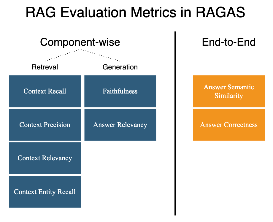
Use RAGAs framework with hyperparameter optimisation to boost the quality of your RAG system.
Graphic depicting the idea of “LLMs Evaluating RAGs”. It was generated by the author with help of AI in Canva.
TL;DR
If you develop a RAG system you need to choose between different design options. This is where the ragas library can help you by generating synthetic evaluation data with answers grounded in your documents. This makes possible the rigorous evaluation of a RAG system with the classic split between train/validation/test sets. As the result the quality of your RAG system will get a big boost.
Introduction
The development of Retrieval Augmented Generation (RAG) system in practice involves taking a lot of decisions that are consequential for its ultimate quality, i.e.: about text splitter, chunk size, overlap size, embedding model, metadata to store, distance metric for semantic search, top-k to rerank, reranker model, top-k to context, prompt engineering, etc.
Reality: In most cases such decisions are not grounded in methodologically sound evaluation practices, but rather driven by ad-hoc judgments of developers and product owners, often facing deadlines.
Gold Standard: In contrast the rigorous evaluation of RAG system should involve:
a large evaluation set, so that performance metrics are estimated with low confidence intervals
diverse questions in an evaluation set
answers specific to the internal documents
separate evaluation of retrieval and generation
evaluation of the RAG as the whole
train/validation/test split to ensure good generalisation ability
hyperparameter optimisation
Most RAG systems are NOT evaluated rigorously up to the Gold Standard due to lack of evaluation sets with answers grounded in the private documents!
The generic Large Language Model (LLM) benchmarks (GLUE, SuperGlue, MMLU, BIG-Bench, HELM, …) are not of much relevance to evaluate RAGs as the essence of RAGs is to extract information from internal documents unknown to LLMs. If you insist to use LLM benchmarks for RAG system evaluation one route would be to select the task specific to your domain, and quantify the value added of the RAG system on top of bare bones LLM for this chosen task.
The alternative to generic LLM benchmarks is to create human annotated test sets based on internal documents, so that the questions require access to these internal documents in order to answer them correctly. In general such a solution is prohibitively expensive in most cases. In addition, outsourcing annotation may be problematic for internal documents, as they are sensitive or contain private information and can’t be shared with outside parties.
Here comes the RAGAs framework (Retrieval Augmented Generation Assessment) [1] for reference-free RAG evaluation, with Python implementation made available in ragas package:
pip install ragas
It provides essential tools for rigorous RAG evaluation:
generation of synthetic evaluation sets
metrics specialised for RAG evaluation
prompt adaptation to deal with non-English languages
integration with LangChain and Llama-Index
Synthetic Evaluation Sets
The LLMs enthusiasts, me included, tend to suggest using LLM as a solution to many problems. Here it means:
LLMs are not autonomous, but may be useful. RAGAs employs LLMs to generate synthetic evaluation sets to evaluate RAG systems.
RAGAs framework follows up on on the idea of Evol-Instruct framework, which uses LLM to generate a diverse set of instruction data (i.e. Question — Answer pairs, QA) in the evolutionary process.
Picture 1: Depicting evolution of questions in RAGAs. . Image created by the author in Canva and draw.io.
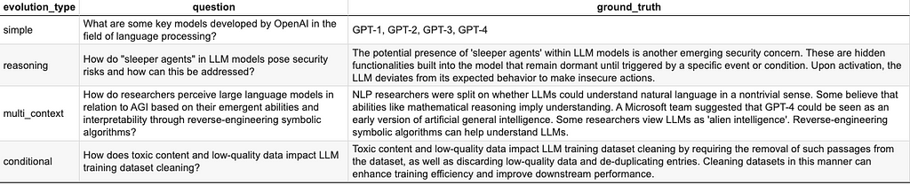
In Evol-Instruct framework LLM starts with an initial set of simple instructions, and gradually rewrites them into more complex instructions, creating a diverse instruction data as the result. Can Xu et al [2] argue that gradual, incremental, evolution instruction data is highly effective in producing high quality results. In RAGAs framework instruction data generated and evolved by LLM are grounded in available documents. The ragas library currently implements three different types of instruction data evolution by depth starting from the simple question:
Reasoning: Rewrite the question to increase the need for reasoning.
Conditioning: Rewrite the question to introduce a conditional element.
Multi-Context: Rewrite the question to requires many documents or chunks to answer it.
In addition ragas library also provides the option to generate conversations. Now let’s see ragas in practice.
Examples of Question Evolutions
We will use the Wikipedia page on Large Language Models [3] as the source document for ragas library to generate question — ground truth pairs, one for each evolution type available.
To run the code: You can follow the code snippets in the article or access the notebook with all the related code on Github to run on Colab or locally:
# Importing the packages
from functools import reduce
import json
import os
import requests
import warnings

import chromadb
from chromadb.api.models.Collection import Collection as ChromaCollection
from datasets import load_dataset, Dataset
from getpass import getpass
from langchain_chroma import Chroma
from langchain_core.prompts import ChatPromptTemplate
from langchain_core.output_parsers import StrOutputParser
from langchain_core.runnables import RunnableParallel, RunnablePassthrough
from langchain_core.runnables.base import RunnableSequence
from langchain_community.document_loaders import WebBaseLoader, PolarsDataFrameLoader
from langchain_openai import ChatOpenAI, OpenAIEmbeddings
from langchain_text_splitters import CharacterTextSplitter
from operator import itemgetter
import optuna
import pandas as pd
import plotly.express as px
import polars as pl
from ragas import evaluate
from ragas.metrics import (
    answer_relevancy,
    faithfulness,
    context_recall,
    context_precision,
    answer_correctness
)
from ragas.testset.generator import TestsetGenerator
from ragas.testset.evolutions import simple, reasoning, multi_context, conditional
# Providing api key for OPENAI
OPENAI_API_KEY = getpass("OPENAI_API_KEY")
os.environ["OPENAI_API_KEY"] = OPENAI_API_KEY
# Displaying examples examples = reduce(lambda x, y: pd.concat([x, y], axis=0), [x.to_pandas() for x in question_evolution_types]) examples = examples.loc[:, ["evolution_type", "question", "ground_truth"]] examples
Running the above code I received the following synthetic question — answer pairs based on the aforementioned Wikipedia page [3].
Table 1: Synthetic question — answer pairs generated using ragas library and GPT-3.5-turbo from the Wikipedia page on LLMs [3].
The results presented in the Table 1 seem very appealing, at least to me. The simple evolution performs very well. In the case of the reasoning evolution the first part of question is answered perfectly, but the second part is left unanswered. Inspecting the Wikipedia page [3] it is evident that there is no answer to the second part of the question in the actual document, so it can also be interpreted as the restraint from hallucinations, a good thing in itself. The multi-context question-answer pair seems very good. The conditional evolution type is acceptable if we look at the question-answer pair. One way of looking at these results is that there is always space for better prompt engineering that are behind evolutions. Another way is to use better LLMs, especially for the critic role as is the default in the ragas library.
Metrics
The ragas library is able to not only generate the synthetic evaluation sets, but also provides us with built-in metrics for component-wise evaluation as well as end-to-end evaluation of RAGs.
As of this writing RAGAS provides out-of-the-box eight metrics for RAG evaluation, see Picture 2, and likely new ones will be added in the future. In general you are about to choose the metrics most suitable for your use case. However, I recommend to select the one most important metric, i.e.:
Answer Correctness— the end-to-end metric with scores between 0 and 1, the higher the better, measuring the accuracy of the generated answer as compared to the ground truth.
Focusing on the one end-to-end metric helps to start the optimisation of your RAG system as fast as possible. Once you achieve some improvements in quality you can look at component-wise metrics, focusing on the most important one for each RAG component:
Faithfulness — the generation metric with scores between 0 and 1, the higher the better, measuring the factual consistency of the generated answer relative to the provided context. It is about grounding the generated answer as much as possible in the provided context, and by doing so prevent hallucinations.
Context Relevance — the retrieval metric with scores between 0 and 1, the higher the better, measuring the relevancy of retrieved context relative to the question.
RAG Factory
OK, so we have a RAG ready for optimisation… not so fast, this is not enough. To optimise RAG we need the factory function to generate RAG chains with given set of RAG hyperparameters. Here we define this factory function in 2 steps:
Step 1: A function to store documents in the vector database.
# Defining a function to get document collection from vector db with given hyperparemeters # The function embeds the documents only if collection is missing # This development version as for production one would rather implement document level check def get_vectordb_collection(chroma_client, documents, embedding_model="text-embedding-ada-002", chunk_size=None, overlap_size=0) -> ChromaCollection:
if chunk_size is None: collection_name = "full_text" docs_pp = documents else: collection_name = f"{embedding_model}_chunk{chunk_size}_overlap{overlap_size}"
existing_collections = [collection.name for collection in chroma_client.list_collections()]
if chroma_client.get_collection(collection_name).count() == 0: langchain_chroma.from_documents(collection_name=collection_name, documents=docs_pp, embedding=embedding) return langchain_chroma
Step 2: A function to generate RAG in LangChain with document collection, or the proper RAG factory function.
# Defininig a function to get a simple RAG as Langchain chain with given hyperparemeters # RAG returns also the context documents retrieved for evaluation purposes in RAGAs
template = """Answer the question based only on the following context. If the context doesn't contain entities present in the question say you don't know.
The former function get_vectordb_collection is incorporated into the latterfunction get_chain, which generates our RAG chain for given set of parameters, i.e: embedding_model, llm_model, chunk_size, overlap_size, top_k, lambda_mult. With our factory function we are just scratching the surface of possibilities what hyperparmeters of our RAG system we optimise. Note also that RAG chain will require 2 arguments: question and ground_truth, where the latter is just passed through the RAG chain as it is required for evaluation using RAGAs.
# Setting up a ChromaDB client
chroma_client = chromadb.EphemeralClient()

# Testing full text rag

with warnings.catch_warnings():
  rag_prototype = get_chain(chroma_client=chroma_client,
                            documents=news,
                            chunk_size=1000,
                            overlap_size=200)

rag_prototype.invoke({"question": 'What happened in Minneapolis to the bridge?',
                      "ground_truth": "x"})["answer"]
RAG Evaluation
To evaluate our RAG we will use the diverse dataset of news articles from CNN and Daily Mail, which is available on Hugging Face [4]. Most articles in this dataset are below 1000 words. In addition we will use the tiny extract from the dataset of just 100 news articles. This is all done to limit the costs and time needed to run the demo.
# Getting the tiny extract of CCN Daily Mail dataset
synthetic_evaluation_set_url = "https://gist.github.com/gox6/0858a1ae2d6e3642aa132674650f9c76/raw/synthetic-evaluation-set-cnn-daily-mail.csv"
synthetic_evaluation_set_pl = pl.read_csv(synthetic_evaluation_set_url, separator=",").drop("index")
# Train/test split # We need at least 2 sets: train and test for RAG optimization.
As we will consider many different RAG prototypes beyond the one define above we need a function to collect answers generated by the RAG on our synthetic evaluation set:
# We create the helper function to generate the RAG ansers together with Ground Truth based on synthetic evaluation set # The dataset for RAGAS evaluation should contain the columns: question, answer, ground_truth, contexts # RAGAs expects the data in Huggingface Dataset format
for row in synthetic_evaluation_set.iter_rows(named=True): rag_output = chain.invoke({"question": row["question"], "ground_truth": row["ground_truth"]}) rag_output["contexts"] = [doc.page_content for doc in rag_output["context"]] del rag_output["context"] rag_output_pp = {k: [v] for k, v in rag_output.items()} df = pl.concat([df, pl.DataFrame(rag_output_pp)], how="vertical")
return df
RAG Optimisation with RAGAs and Optuna
First, it is worth emphasising that the proper optimisation of RAG system should involve global optimisation, where all parameters are optimised at once, in contrast to the sequential or greedy approach, where parameters are optimised one by one. The sequential approach ignores the fact that there can be interactions between the parameters, which can result in sub-optimal solution.
Now at last we are ready to optimise our RAG system. We will use hyperparameter optimisation framework Optuna. To this end we define the objective function for the Optuna’s study specifying the allowed hyperparameter space as well as computing the evaluation metric, see the code below:
Finally, having the objective function we define and run the study to optimise our RAG system in Optuna. It’s worth noting that we can add to the study our educated guesses of hyperparameters with the method enqueue_trial, as well as limit the study by time or number of trials, see the Optuna’s docs for more tips.
sampler = optuna.samplers.TPESampler(seed=6) study = optuna.create_study(study_name="RAG Optimisation", direction="maximize", sampler=sampler) study.set_metric_names(['answer_correctness'])
print(f"Sampler is {study.sampler.__class__.__name__}") study.optimize(objective, timeout=180)
In our study the educated guess wasn’t confirmed, but I’m sure that with rigorous approach as the one proposed above it will get better.
Best trial with answer_correctness: 0.700130617593832
Hyper-parameters for the best trial: {'embedding_model': 'text-embedding-ada-002', 'chunk_size': 700, 'overlap_size': 400, 'top_k': 9}
Limitations of RAGAs
After experimenting with ragas library to synthesise evaluations sets and to evaluate RAGs I have some caveats:
The question may contain the answer.
The ground-truth is just the literal excerpt from the document.
Issues with RateLimitError as well as network overflows on Colab.
Built-in evolutions are few and there is no easy way to add new, ones.
There is room for improvements in documentation.
The first 2 caveats are quality related. The root cause of them may be in the LLM used, and obviously GPT-4 gives better results than GPT-3.5-Turbo. At the same time it seems that this could be improved by some prompt engineering for evolutions used to generate synthetic evaluation sets.
As for issues with rate-limiting and network overflows it is advisable to use: 1) checkpointing during generation of synthetic evaluation sets to prevent loss of of created data, and 2) exponential backoff to make sure you complete the whole task.
Finally and most importantly, more built-in evolutions would be welcome addition for the ragas package. Not to mention the possibility of creating custom evolutions more easily.
Other Useful Features of RAGAs
Custom Prompts. The ragas package provides you with the option to change the prompts used in the provided abstractions. The example of custom prompts for metrics in the evaluation task is described in the docs. Below I use custom prompts for modifying evolutions to mitigate quality issues.
Automatic Language Adaptation. RAGAs has you covered for non-English languages. It has a great feature called automatic language adaptation supporting RAG evaluation in the languages other than English, see the docs for more info.
Conclusions
Despite RAGAs limitations do NOT miss the most important thing:
RAGAs is already very useful tool despite its young age. It enables generation of synthetic evaluation set for rigorous RAG evaluation, a critical aspect for successful RAG development.
If you enjoyed reading this article consider helping me promote it to the other readers, please clap or respond. I invite You to look atmy other articles!Consider subscribing to my new content.
Acknowledgements
Obviously this project & article would be impossible if I didn’t stand on the shoulders of giants. It is impossible to mention all influences, but the following were directly related:
[1] S. Es, J. James, L. Espinosa-Anke, S. Schockaert, RAGAS: Automated Evaluation of Retrieval Augmented Generation (2023), arXiv:2309.15217
[2] C. Xu, Q. Sun, K. Zheng, X. Geng, P. Zhao, J. Feng, C. Tao, D. Jiang, WizardLM: Empowering Large Language Models to Follow Complex Instructions (2023), arXiv:2304.12244
This post describes some interesting processes for transforming the map boundaries in vector datasets using QGIS and geopandas in Python.
Recently, for one of my projects, I had to define the composition of countries in a region, make the region distinct, and highlight it on the map of a continent. Let’s take an example of the South Asia region in Asia. The South Asia region is comprised of eight countries: Afghanistan, Bangladesh, Bhutan, India, Maldives, Nepal, Pakistan and Sri Lanka. From the map of Asia, I wanted to clip off the South Asia region and highlight it distinctly in the continental map. Furthermore, I wanted to go one step ahead and dissolve the boundaries of the countries in the region so that the region could be demonstrated as a single unit.
I was able to achieve this using both Quantum-GIS (QGIS) and geopandas package in Python. In this process, I utilized the clipping feature which I was already familiar with, and I learned about the dissolve feature which I found very fascinating. In this post, I am going to share my learning about these features and how I achieved my objectives. Let’s get started.
Image by Author.
1. QGIS
In an empty QGIS project, by typing world in the coordinate space in the bottom of the page, I could call an in-built map of the world with administrative boundaries of all the countries as shown below.
Getting a world map in QGIS. Image by Author.
Next, by using the select feature, I selected the 8 countries of South Asia as highlighted in the map below. QGIS offers the option to select countries by hand, by polygon, by radius, and by individually selecting or deselecting countries with a mouse click.
Selecting countries from the world map. Image by Author.
Clipping in QGIS
Clipping these countries off of the world map is straightforward in QGIS. One needs to go to Vector in the menu-> Select Geoprocessing tools -> Select Clip. In the options, I ticked on the check box for the Selected features only in the Input layer and ran the process.
Running Clipping algorithm. Image by Author.
The clipping action was completed in 7.24 seconds alone and I got a new layer called “Clipped”. This is depicted by the brown color in the screenshot below. By going to Properties of the layer, one can use different coloring options in QGIS in the Symbology option.
New Clipped layer is created. Image by Author.
Dissolving boundaries in QGIS
Next, I wanted to dissolve the boundaries between countries in South Asia. For this, I selected all the countries in South Asia. I went to the Vector Menu -> Select Geoprocessing Tools ->Dissolve. Similar to the previous step, I selected “Selected featured only” in the input layer and ran the algorithm which took just 0.08 seconds. A new layer called “Dissolved” was created where the administrative boundaries between countries were dissolved and appeared as a single unit as shown below:
New Dissolved layer is created. Image by Author.
Visualizing both the world layer and Dissolved layer at the same time looks as shown below:
Dissolved layer and world layer. Image by Author.
2. Geopandas
In this section, I am going to demonstrate how I could the same objective in Python using the geopandas package.
In the first step, I read the in-built dataset of the world map within the geopandas package. It contains the vector data of the world with the administative boundaries of all counntries. This is obtained from the Natural Earth dataset, which is free to use.
import pandas as pd
import geopandas as gpd
import matplotlib.pyplot as plt
import numpy as np

world = gpd.read_file(gpd.datasets.get_path('naturalearth_lowres'))
world.plot(color = "lightgrey")
Plotting world map in geopandas. Image by Author.
Clipping with geopandas
In my very first post, I demonstrated how it is possible to clip off a custom Polygon geometry as a mask from the original geopandas dataframe or layer. However, for simplicity, I just used the filter options to obtain the required layers for Asia and South Asia.
asia = world[world.continent == "Asia"]
asia.plot(color = "lightgrey")
Filtering Asia continent from world. Image by Author.
To filter the South Asia region, I used a list containing the name of each country as a reference.
Filtering South Asia region from Asia. Image by Author.
Dissolve boundaries between countries in South Asia using geopandas
To dissolve the boundaries between countries in South Asia, I used the dissolve feature in geopandas. I passed None as an argument, and specified parameters to apply certain aggregate functions, in which the population and GDP in the resulting dissolved dataframe would sum up the population and GDP in all countries in South Asia. I am yet to figure out how the aggregate function can also be applied in QGIS.
Administrative boundaries between countries in South Asia are dissolved. Image by Author.
Dissolving boundaries between countries within a continent in the world
Using the same procedure as above, I wanted to dissolve the boundaries between countries within a continent and show different continents distinct from each other in a world map based on the number of countries in each continent.
For this purpose, first I added a new column called num_countries in the world geodataframe containing 1 as a value. Then I dissolved the world map using the continent column as a reference.
I used the aggregate function to sum up the population and GDP in all countries in the continent and count the number of countries in each continent. The resulting geodataframe continents_dissolved look as shown:
We see that Asia has the largest population and GDP of all continents. Similarly, we see that Africa has the most countries (51) followed by Asia (47), Europe (39), North America (18), South America (13), and Oceania (7). Antarctica and Seven seas (open ocean) are also regarded as continents in this dataset.
Finally, I wanted to plot the world map highlighting the number of countries in each continent with the help of a color map. I achieved this using the following code:
# Add a horizontal colorbar cbar = plt.colorbar(map.get_children()[0], ax=ax, orientation='horizontal', aspect = 30 #control the width of color bar. higher value= lower width. )
# Set a label for the colorbar cbar.set_label('Number of Countries')
plt.title("Continents of the world based on number of countries")
Map of the world where the color reflects number of countries in each continent. Image by Author.
Conclusion
In this post, I described ways to dissolve map boundaries using QGIS and geopandas in Python. In the process, I also explained the clipping process and the possibility of using aggregate function while dissolving the map boundaries in geopandas. These processes could be very useful for the manipulation, processing, and transformation of geographical maps in the form of vector datasets. The code and the QGIS project file for this post are available in this GitHub repository. Thank you for reading!
Hansen (1982) pioneered the introduction of the generalized method of moments (GMM), making notable contributions to empirical research in finance, particularly in asset pricing. The creation of the model was motivated by the need to estimate parameters in economic models while adhering to the theoretical constraints implicit in the model. For example, if the economic model states that two things should be independent, the GMM will try to find a solution in which the average of their product is zero. Therefore, understanding GMM can be a powerful alternative for those who need a model in which theoretical conditions are extremely important, but which conventional models cannot satisfy due to the nature of the data.
Concepts
This estimation technique is widely used in econometrics and statistics to address endogeneity and other issues in regression analysis. The basic concept of the GMM estimator involves minimizing a criterion function by choosing parameters that make the sample moments of the data as close as possible to the population moments. The equation for the Basic GMM Estimator can be expressed as follows:
The GMM estimator aims to find the parameter vector θ that minimizes this criterion function, thereby ensuring that the sample moments of the data align as closely as possible with the population moments. By optimizing this criterion function, the GMM estimator provides consistent estimates of the parameters in econometric models.
Being consistent means that as the sample size approaches infinity, the estimator converges in probability to the true parameter value (asymptotically normal). This property is crucial for ensuring that the estimator provides reliable estimates as the amount of data increases. Even in the presence of omitted variables, as long as the moment conditions are valid and instruments are correctly specified, GMM can provide consistent estimators. However, the omission of relevant variables can impact the efficiency and interpretation of the estimated parameters.
To be efficient, GMM utilizes Generalized Least Squares (GLS) on Z-moments to improve the precision and efficiency of parameter estimates in econometric models. GLS addresses heteroscedasticity and autocorrelation by weighting observations based on their variance. In GMM, Z-moments are projected into the column space of instrumental variables, similar to a GLS approach. This minimizes variance and enhances parameter estimate precision by focusing on Z-moments and applying GLS techniques.
Assumptions
However, it is important to recognize that the GMM estimator is subject to a series of assumptions that must be considered during its application, which have been listed:
Existence of Moments: Up to a certain order is necessary and requires finite tails in the distribution of the data.
Correct Model Specification: The underlying model must be correctly specified, including the functional relationship and the distribution of error terms.
Identifiability: There must be a unique solution for the parameters to be estimated.
Moment Conditions: It is necessary to specify the moment conditions correctly, which must have zero mean under the model assumptions.
Valid Instruments: If applicable, instruments must be relevant and valid.
Independence and Homoscedasticity (conditional): Ideally, errors should be independent and homoscedastic under the moment conditions.
Robustness to Heteroscedasticity: GMM is robust to heteroscedasticity if the weighting matrix is consistently estimated.
Multicollinearity: GMM can handle multicollinearity, but it can affect the efficiency of the estimators.
Outliers: GMM is sensitive to outliers unless they are properly addressed in the modeling process.
Large Samples: GMM is more efficient in large samples.
Asymptotic Theory: Properties such as consistency and efficiency are asymptotic.
When to use
Therefore, GMM is a highly flexible estimation technique and can be applied in a variety of situations, being widely used as a parameter estimation technique in econometrics and statistics. It allows for efficient estimation of parameters under different model specifications and data structures. Its main uses are:
Models with Instrumental Variables: used when there are endogenous variables in a model. It provides a way to correct bias in parameter estimation when explanatory variables are correlated with the error.
Models with Measurement Errors: GMM can be used to correct bias introduced by measurement errors in variables.
Models with Moment Restrictions: In some situations, there are multiple moment conditions that a model must satisfy. GMM allows you to use all this information simultaneously for more efficient estimation.
Time Series Models: GMM is often applied in ARMA (AutoRegressive Moving Average) models and other time series models.
Panel Data Models: It can be used in panel data models to handle issues like heteroscedasticity and autocorrelation within cross-sectional units.
Nonlinear Models: GMM is also extendable to nonlinear models, providing a robust estimation technique when classical methods like Maximum Likelihood may be infeasible.
Comparing to OLS
The contrast between the Ordinary Least Squares (OLS) method and the Generalized Method of Moments (GMM) points out different advantages. OLS proves itself efficient under the classical assumptions of linearity, serving as an unbiased linear estimator of minimum variance (BLUE). The fundamental assumptions of a linear regression model include: linearity in the relationship between variables, absence of perfect multicollinearity, zero mean error, homoscedasticity (constant variance of errors), non-autocorrelation of errors and normality of errors. Therefore, OLS is an unbiased, consistent and efficient estimator. Furthermore, it have relatively lower computational complexity.
However, GMM provides more flexibility, which is applicable to a wide range of contexts such as models with measurement errors, endogenous variables, heteroscedasticity, and autocorrelation. It makes no assumptions about the distribution of errors and is applicable to nonlinear models. GMM stands out in cases where we have omitted important variables, multiple moment conditions, nonlinear models, and datasets with heteroscedasticity and autocorrelation.
Comparing to MLE
Conversely, when comparing GMM and Maximum Likelihood Estimation (MLE), it highlights their approaches to handling data assumptions. GMM constructs estimators using data and population moment conditions, providing flexibility and adaptability to models with fewer assumptions, particularly advantageous when strong assumptions about data distribution may not hold.
MLE estimates parameters by maximizing the likelihood of the given data, depending on specific assumptions about data distribution. While MLE performs optimally when the assumed distribution closely aligns with the true data-generating process, GMM accommodates various distributions, proving valuable in scenarios where data may not conform to a single specific distribution.
Estimation in Python
In the hypothetical example demonstrated in Python, we utilize the linearmodels.iv library to estimate a GMM model with the IVGMM function. In this model, consumption serves as the dependent variable, while age and gender (represented as a dummy variable for male) are considered exogenous variables. Additionally, we assume that income is an endogenous variable, while the number of children and education level are instrumental variables.
import pandas as pd from linearmodels.iv import IVGMM
# Read the Excel file df = pd.read_excel('example.xlsx')
# Construct the formula for GMM formula = "{dep} ~ 1 + {exog} + [{endog} ~ {instr}]".format( dep=dependent, exog='+'.join(exog_vars), endog=endog_vars[0], instr='+'.join(instruments) )
# Estimate the GMM model model = IVGMM.from_formula(formula, df) result = model.fit(cov_type='robust')
# Displaying GMM results print(result)
Instrumental variables in GMM models are used to address endogeneity issues by providing a source of exogenous variation that is correlated with the endogenous regressors but uncorrelated with the error term. The IVGMM function is specifically designed for estimating models in which instrumental variables are used within the framework of GMM.
Therefore, by specifying Consumption as the dependent variable and employing exogenous variables (age and gender) along with instrumental variables (number of children and education) to address endogeneity, this example fits within the GMM context.
In conclusion, the Generalized Method of Moments (GMM) is seen as a powerful and versatile technique in both econometric and statistical applications, giving it a certain advantage over other methods in some cases. In contrast to the traditional OLS and MLE methods, this method allows for a wider range of model specifications and data structures, as it is less restricted in the assumptions that are required to be satisfied.
In cases of endogeneity, measurement errors, momentum constraints, GMM is especially advantageous. Furthermore, the model performs better in the presence of non-linearities and issues of heteroscedasticity and autocorrelation in the data. GMM utilizes moment conditions and instrumental variables that provide consistent and efficient parameter estimates and is therefore a great alternative of choice for empirical researchers where theoretical conditions are critically important and common methods are not applicable due to violated assumptions or complex data structures.
Therefore, GMM becomes a versatile measurement tool that is suitable for a wide range of empirical settings, allowing researchers to adequately handle complex modeling tasks and provide correct estimates of model parameters.
References
Hansen, L. P. (1982). Large Sample Properties of Generalized Method of Moments Estimators. Econometrica, 50(4), 1029–1054. https://doi.org/10.2307/1912775
We use cookies on our website to give you the most relevant experience by remembering your preferences and repeat visits. By clicking “Accept”, you consent to the use of ALL the cookies.
This website uses cookies to improve your experience while you navigate through the website. Out of these, the cookies that are categorized as necessary are stored on your browser as they are essential for the working of basic functionalities of the website. We also use third-party cookies that help us analyze and understand how you use this website. These cookies will be stored in your browser only with your consent. You also have the option to opt-out of these cookies. But opting out of some of these cookies may affect your browsing experience.
Necessary cookies are absolutely essential for the website to function properly. These cookies ensure basic functionalities and security features of the website, anonymously.
Cookie
Duration
Description
cookielawinfo-checkbox-analytics
11 months
This cookie is set by GDPR Cookie Consent plugin. The cookie is used to store the user consent for the cookies in the category "Analytics".
cookielawinfo-checkbox-functional
11 months
The cookie is set by GDPR cookie consent to record the user consent for the cookies in the category "Functional".
cookielawinfo-checkbox-necessary
11 months
This cookie is set by GDPR Cookie Consent plugin. The cookies is used to store the user consent for the cookies in the category "Necessary".
cookielawinfo-checkbox-others
11 months
This cookie is set by GDPR Cookie Consent plugin. The cookie is used to store the user consent for the cookies in the category "Other.
cookielawinfo-checkbox-performance
11 months
This cookie is set by GDPR Cookie Consent plugin. The cookie is used to store the user consent for the cookies in the category "Performance".
viewed_cookie_policy
11 months
The cookie is set by the GDPR Cookie Consent plugin and is used to store whether or not user has consented to the use of cookies. It does not store any personal data.
Functional cookies help to perform certain functionalities like sharing the content of the website on social media platforms, collect feedbacks, and other third-party features.
Performance cookies are used to understand and analyze the key performance indexes of the website which helps in delivering a better user experience for the visitors.
Analytical cookies are used to understand how visitors interact with the website. These cookies help provide information on metrics the number of visitors, bounce rate, traffic source, etc.
Advertisement cookies are used to provide visitors with relevant ads and marketing campaigns. These cookies track visitors across websites and collect information to provide customized ads.