And why the path to real intelligence goes through ontologies and knowledge graphs
Those who follow me, might remember a similar AI rant from a year ago, under the pseudonym “Grumpy Risk Manager”. Now I’m back, grumpier than ever, with specific examples but also ideas for solutions!
Source: author collage
Introduction
Large Language Models (LLMs) like ChatGPT are impressive in their ability to discuss generic topics in natural language.
However, they struggle in specialist domains such as medicine, finance and law.
This is due to lack of real understanding and focus on imitation rather than intelligence.
LLMs are at the peak of their hype. They are considered “intelligent” due to their ability to answer and discuss generic topics in natural language.
However, once you dive into a specialist/complex domains such as medicine, finance, law, it is easy to observe logical inconsistencies, plain mistakes and the so called “hallucinations”. To put it simply, the LLM behaves like a pupil with a very rich dictionary who tries to pretend that they’ve studied for the exam and know all the answers, but they actually don’t! They just pretend to be intelligent due to the vast information at their disposal, but their ability to reason using this information is very limited. I would even go a step further and say that:
The so-called Artificial Intelligence (AI) is very often Artificial Imitation of Intelligence (AII). This is particularly bad in specialist domains like medicine or finance, since a mistake there can lead to human harm and financial losses.
Let me give you a real example from the domain in which I’ve spent the last 10 years — financial risk. Good evidence of it being “specialist” is the amount of contextual information that has to be provided to the average person in order to understand the topic:
Banks are subject to regulatory Capital requirements.
Capital can be considered a buffer which absorbs financial losses.
The requirements to hold Capital, ensures that banks have sufficient capability to absorb losses reducing the likelihood of bankruptcy and financial crisis.
The rules for setting the requirements in 1. are based on risk-proportionality principles: → the riskier the business that banks undertake → higher risk-weights → higher capital requirements → larger loss buffer → stable bank
The degree of riskiness in 4. is often measured in the form of credit rating of the firms with which the bank does business.
Credit ratings come from different agencies and in different formats.
In order to standardise the ratings, regulators have created mapping rules from every rating format to the standardised Credit Quality Step (CQS) in the range of 1 to 6.
Then the regulatory rules for determining the risk-weights in 4. are based on the CQS.
The rules in 8. for European banks are set in the Capital Requirements Regulation (CRR).
The topic in the 9 statements above seems complex and it really is, there are dozens of additional complications and cases that exist, but which I’ve avoided on purpose, as they are not even necessary for illustrating the struggle of AII with such topics. Furthermore, the complexity doesn’t arise from any of the individual 9 rules itself, but rather from their combination, there are a lot of concepts whose definition is based on several other concepts giving rise to a semantic net/graph of relationships connecting the concepts and the rules.
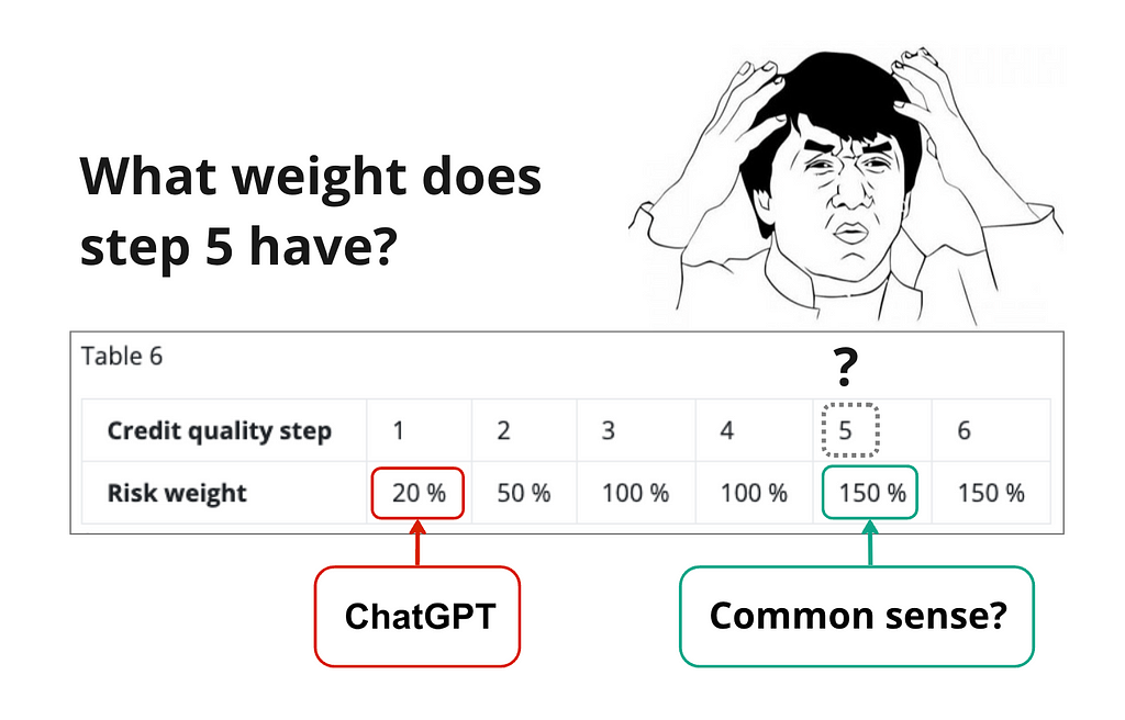
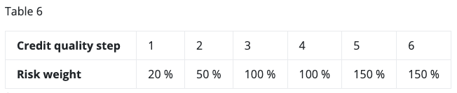
Now let’s focus only on the core concepts and rules in 4, which can be summarised as follows: rating → CQS → risk-weight → capital requirement. If we also look at an example CRR article 122, we can see a mapping table CQS → risk-weight which should be used for corporate exposures.
Capital Requirements Regulation (CRR 122)
This mapping rule is very simple, it can be understood easily by the average person with a bit of context. It is also known by many banking specialists and most of them don’t memorise the exact rule but simply know the information of the 9 statements above and know where to look in order to see the exact mapping.
Artificially Imitated Intelligence
Now let’s formulate a question and see whether AII can deal with it, here is what I asked ChatGPT 3.5:
According to CRR, what is the risk-weight of an exposure to corporate which has credit quality step of 5?
And here is the answer:
In the Capital Requirements Regulation (CRR), the risk-weight of an exposure to a corporate entity depends on its credit quality step. In the context of credit quality steps, a credit quality step of 5 typically represents the highest credit quality, indicating a very low risk of default.
In the standardised approach outlined in the CRR, exposures to corporates are assigned risk weights based on their credit ratings or credit quality steps. The risk weights for exposures to corporates range from 20% to 150%, depending on the credit quality step and whether the exposure is short-term or long-term.
Since a credit quality step of 5 signifies a very low risk, the corresponding risk weight assigned to such an exposure would be one of the lowest. In this case, for a corporate with a credit quality step of 5, the risk weight would likely be 20% or similar, indicating a low capital requirement for banks holding such exposures.
Can you spot the factual mistakes, highlighted in bold?
First very big mistake is that the AII completely misunderstood and inverted the CQS → risk-weight relationship, high CQS of 5 doesn’t represent low risk but exactly the opposite, it is one of the highest risks! This is actually the biggest mistake one could possibly make when answering this question!
Even after the mistake in 1, I would expect the AII to be able to look-up a table in an article and conclude that below a CQS of 5, there is a risk-weight of 150%. But no, the AII confidently claims 20% risk-weight, due to low risk…
Although undeserved, I still gave the benefit of doubt to the AII, by asking the same question but clarifying the exact CRR article: 122. Shameless, but confident, the AII now responded that the risk-weight should be 100%, still claiming that CQS of 5 is good credit quality → another obvious mistake.
Feeling safe for my job and that the financial industry still needs me, I started thinking about solutions, which ironically could make my job unsafe in the future…
Why ontologies and knowledge graphs?
Enter ontologies, a form of knowledge representation of a particular domain. One good way of thinking about it, is in terms of ordering the different ways of representing knowledge from least to more sophisticated:
Data dictionary: table with field names and metadata attributes
Taxonomy: table/s with added nesting of data types and sub-types in terms of relationships (e.g. Pigeon <is a type of> Bird)
Ontology: Multidimensional taxonomies with more than one type of relationships (e.g. Birds <eat> Seeds) “the unholy marriage of a taxonomy with object oriented programming” (Kurt Cagle, 2017)
Why would one want to incorporate such complex relational structure in their data? Below are the benefits which will be later illustrated with an example:
Uniform representation of: structure, data and logic. In the example above, Bird is a class which is a template with generic properties = structure. In an ontology, we can also define many actual instances of individual Birds with their own properties = data. Finally, we can also add logic (e.g. If a Bird <eats> more than 5 Seeds, then <it is> not Hungry). This is essentially making the data “smart” by incorporating some of the logic as data itself, thus making it a reusable knowledge. It also makes information both human and machine readable which is particularly useful in ML.
Explainability and Lineage: most frequent implementation of ontology is via Resource Description Framework (RDF) in the form of graphs. These graphs can then be queried in order to evaluate existing rules and instances or add new ones. Moreover, the chain of thought, through the graph nodes and edges can be traced, explaining the query results and avoiding the ML black box problem.
Reasoning and Inference: when new information is added, a semantic reasoner can evaluate the consequences on the graph. Moreover, new knowledge can be derived from existing one via “What if” questions.
Consistency: any conflicting rules or instances that deviate from the generic class properties are automatically identified as an error by the reasoner and cannot become part of the graph. This is extremely valuable as it enforces agreement of knowledge in a given area, eliminating any subjective interpretations.
Interoperability and Scalability: the reusable knowledge can focus on a particular specialist domain or connect different domains (see FIBO in finance, OntoMathPRO in maths, OGMS in medicine). Moreover, one could download a general industry ontology and extend it with private enterprise data in the form of instances and custom rules.
Ontologies can be considered one of the earliest and purest forms of AI, long before large ML models became a thing and all based on the idea of making data smart via structuring. Here by AI, I mean real intelligence — the reason the ontology can explain the evaluated result of a given rule is because it has semantic understanding about how things work! The concept became popular first under the idea of Semantic Web in the early 2000s, representing the evolution of the internet of linked data (Web 3.0), from the internet of linked apps (Web 2.0) and the internet of linked pages (Web 1.0).
Knowledge Graphs (KGs) are a bit more generic term for the storage of data in graph format, which may not necessarily follow ontological and semantic principles, while the latter are usually represented in the form of a KG. Nowadays, with the rise of LLMs, KGs are often seen as a good candidate for resolving their weaknesses in specialist domains, which in turn revives the concept of ontologies and their KG representation.
This leads to very interesting convergence of paradigms:
Ontologies aim to generate intelligence through making the data smart via structure.
LLMs aim to generate intelligence through leaving the data unstructured but making the model very large and structural: ChatGPT has around 175 billion parameters!
Clearly the goal is the same, and the outcome of whether the data becomes part of the model or the model becomes part of the data becomes simply a matter of reference frame, inevitably leading to a form of information singularity.
Why use ontologies in banking?
Specialisation: as shown above, LLMs struggle in specialist fields such as finance. This is particularly bad in a field in which mistakes are costly. In addition, value added from automating knowledge in specialist domains that have fewer qualified experts can be much higher than that of automation in generic domains (e.g. replacing banking expert vs support agent).
Audit trail: when financial items are evaluated and aggregated in a financial statement, regulators and auditors expect to have continuous audit trail from all granular inputs and rules to the final aggregate result.
Explainability: professionals rely on having a good understanding of the mechanisms under which a bank operates and impact of risk drivers on its portfolios and business decisions. Moreover, regulators explicitly require such understanding via regular “What if” exercises in the form of stress testing. This is one of the reasons ML has seen poor adoption in core banking — the so-called black box problem.
Objectivity and Standardisation: lack of interpretation and subjectivity ensures level playing field in the industry, fair competition and effectiveness of the regulations in terms of ensuring financial stability.
Now imagine a perfect world in which regulations such as the CRR are provided in the form of ontology rather than free text.
Each bank can import the ontology standard and extend it with its own private data and portfolio characteristics, and evaluate all regulatory rules.
Furthermore, the individual enterprise strategy can be also combined with the regulatory constraints in order to enable automated financial planning and optimised decision making.
Finally, the complex composite impacts of the big graph of rules and data can be disentangled in order to explain the final results and give insights into previously non-obvious relationships.
The below example aims to illustrate these ideas on a minimal effort, maximum impact basis!
Example
On the search for solutions of the illustrated LLM weaknesses, I designed the following example:
Create an ontology in the form of a knowledge graph.
Define the structure of entities, add individual instances/data and logic governing their interactions, following the CRR regulation.
Use the knowledge graph to evaluate the risk-weight.
Ask the KG to explain how it reached this result.
For creating the simple ontology, I used the CogniPy library with the main benefits of:
Using Controlled Natural Language (CNL) for both writing and querying the ontology, meaning no need to know specific graph query languages.
Visualisation of the materialised knowledge graphs.
Reasoners with ability to explain results.
Structure
First, let’s start by defining the structure of our ontology. This is similar to defining classes in objective oriented programming with different properties and constraints.
In the first CNL statement, we define the company class and its properties.
Every company has-id one (some integer value) and has-cqs one (some integer value) and has-turnover (some double value).
Several things to note is that class names are with small letter (company). Different relationships and properties are defined with dash-case, while data types are defined in the brackets. Gradually, this starts to look more and more like a fully fledged programming language based on plain English.
Next, we illustrate another ability to denote the uniqueness of the company based on its id via generic class statement.
Every X that is a company is-unique-if X has-id equal-to something.
Data
Now let’s add some data or instances of the company class, with instances starting with capital letter.
Lamersoft is a company and has-id equal-to 123 and has-cqs equal-to 5 and has-turnover equal-to 51000000.
Here we add a data point with a specific company called Lamersoft, with assigned values to its properties. Of course, we are not limited to a single data point, we could have thousands or millions in the same ontology and they can be imported with or without the structure or the logic components.
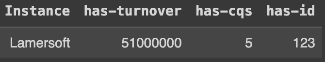
Now that we’ve added data to our structure, we can query the ontology for the first time to get all companies, which returns a DataFrame of instances matching the query:
onto.select_instances_of("a thing that is a company")
DataFrame with query results
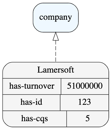
We can also plot our knowledge graph, which shows the relationship between the Lamersoft instance and the general class company:
onto.draw_graph(layout='hierarchical')
Ontology graph
Logic
Finally, let’s add some simple rules implementing the CRR risk-weight regulations for corporates.
If a company has-turnover greater-than 50000000 then the company is a corporate.
If a corporate has-cqs equal-to 5 then the corporate has-risk-weight equal-to 1.50.
The first rule defines what a corporate is, which usually is a company with large turnover above 50 million. The second rule implements part of the CRR mapping table CQS → risk-weight which was so hard to understand by the LLM.
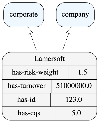
After adding the rules, we’ve completed our ontology and can plot the knowledge graph again:
Ontology graph with evaluated rules
Notably, 2 important deductions have been made automatically by the knowledge graph as soon as we’ve added the logic to the structure and data:
Lamersoft has been identified as a corporate due to its turnover property and the corporate classification rule.
Lamersoft’s risk-weight has been evaluated due to its CQS property and the CRR rule.
This is all as a result of the magical automated consistency (no conflicts) of all information in the ontology. If we were to add any rule or instance that contradicts any of the existing information we would get an error from the reasoner and the knowledge graph would not be materialised.
Now we can also play with the reasoner and ask why a given evaluation has been made or what is the chain of thought and audit trail leading to it:
printWhy(onto,"Lamersoft is a corporate?")
{
  "by": [
    {
      "expr": "Lamersoft is a company."
    },
    {
      "expr": "Lamersoft has-turnover equal-to 51000000."
    }
  ],
  "concluded": "Lamersoft is a corporate.",
  "rule": "If a company has-turnover greater-than 50000000 then the company is a corporate."
}
Regardless of the output formatting, we can still clearly read that by the two expressions defining Lamersoft as a company and its specific turnover, it was concluded that it is a corporate because of the specific turnover condition. Unfortunately, the current library implementation doesn’t seem to support an explanation of the risk-weight result, which is food for the future ideas section.
Nevertheless, I deem the example successful as it managed to unite in a single scalable ontology, structure, data and logic, with minimal effort and resources, using natural English. Moreover, it was able to make evaluations of the rules and explain them with a complete audit trail.
One could say here, ok what have we achieved, it is just another programming language closer to natural English, and one could do the same things with Python classes, instances and assertions. And this is true, to the extent that any programming language is a communication protocol between human and machine. Also, we can clearly observe the trend of the programming syntaxes moving closer to the human language, from the Domain Driven Design (DDD) focusing on implementing the actual business concepts and interactions, to the LLM add-ons of Integrated Development Environments (IDEs) to generate code from natural language. This becomes a clear trend:
The role of programmers as intermediators between the business and the technology is changing. Do we need code and business documentation, if the former can be generated directly from the natural language specification of the business problem, and the latter can be generated in the form of natural language definition of the logic by the explainer?
Conclusion
Imagine a world in which all banking regulations are provided centrally by the regulator not in the form of text but in the form of an ontology or smart data, that includes all structure and logic. While individual banks import the central ontology and extend it with their own data, thus automatically evaluating all rules and requirements. This will remove any room for subjectivity and interpretation and ensure a complete audit trail of the results.
Beyond regulations, enterprises can develop their own ontologies in which they encode, automate and reuse the knowledge of their specialists or different calculation methodologies and governance processes. On an enterprise level, such ontology can add value for enforcing a common dictionary and understanding of the rules and reduce effort wasted on interpretations and disagreements which can be redirected to building more knowledge in the form of ontology. The same concept can be applied to any specialist area in which:
Text association is not sufficient and LLMs struggle.
Big data for effective ML training is not available.
Highly-qualified specialists can be assisted by real artificial intelligence, reducing costs and risks of mistakes.
If data is nowadays deemed as valuable as gold, I believe that the real diamond is structured data, that we can call knowledge. Such knowledge in the form of ontologies and knowledge graphs can also be traded between companies just like data is traded now for marketing purposes. Who knows, maybe this will evolve into a pay-per-node business model, where expertise in the form of smart data can be sold as a product or service.
Then we can call intelligence our ability to accumulate knowledge and to query it for getting actionable insights. This can evolve into specialist AIs that tap into ontologies in order to gain expertise in a given field and reduce hallucinations.
Note however the exact area of application of the LLM! This is not the more specialised fields of financial/product planning or asset and liabilities management of a financial company such as Klarna. It is the general customer support service, which is the entry level position in many companies, which already uses a lot of standardised responses or procedures. The area in which it is easiest to apply AI but also in which the value added might not be the largest. In addition, the risk of LLM hallucination due to lack of real intelligence is still there. Especially in the financial services sector, any form of “financial advice” by the LLM can lead to legal and regulatory repercussions.
Future ideas
LLMs already utilise knowledge graphs in the so-called Retrieval-Augmented Generation (RAG). However, these graphs are generic concepts that might include any data structure and do not necessarily represent ontologies, which use by LLMs is relatively less explored. This gives me the following ideas for next article:
Use plain English to query the ontology, avoiding reliance on particular CNL syntax — this can be done via NLP model that generates queries to the knowledge graph in which the ontology is stored — chatting with KGs.
Use a more robust way of generating the ontology — the CogniPy library was useful for quick illustration, however, for extended use a more proven framework for ontology-oriented programming should be used like Owlready2.
Point 1. enables the general user to get information from the ontology without knowing any programming, however, point 2 implies that a software developer is needed for defining and writing to the ontology (which has its pros and cons). However, if we want to close the AI loop, then specialists should be able to define ontologies using natural language and without the need for developers. This will be harder to do, but similar examples already exist: LLM with KG interface, entity resolution.
A proof of concept that achieves all 3 points above can claim the title of true AI, it should be able to develop knowledge in a smart data structure which is both human and machine readable, and query it via natural language to get actionable insights with complete transparency and audit trail.
Efficient geodata management for optimized search in real-world applications
Introduction
Google Maps and Uber are only some examples of the most popular applications working with geographical data. Storing information about millions of places in the world obliges them to efficiently store and operate on geographical positions, including distance calculation and search of the nearest neighbours.
All modern geographical applications use 2D locations of objects represented by longitude and latitude. While it might seem naive to store the geodata in the form of coordinate pairs, there are some pitfalls in this approach.
In this article, we will discuss the underlying issues of the naive approach and talk about another modern format used to accelerate data manipulation in large systems.
Note. In this article, we will represent the world as a large flat 2D rectangle instead of a 3D ellipse. Longitude and latitude will be represented by X and Y coordinates respectively. This simplification will make the explanation process easier without omitting the main details.
Problem
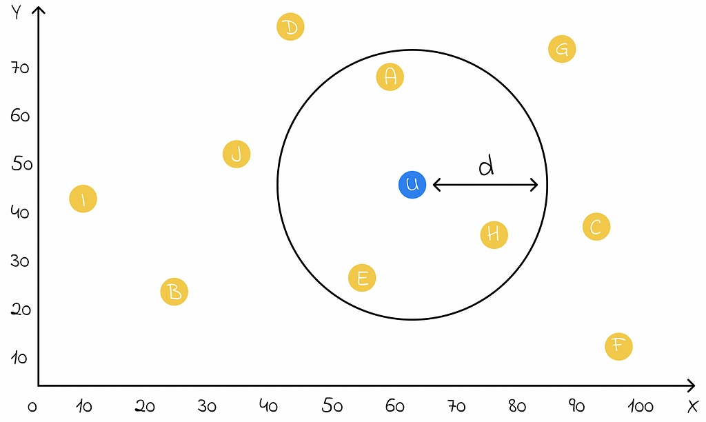
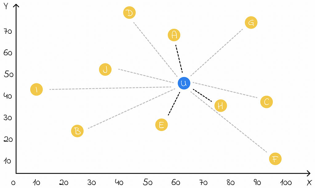
Let us imagine a database storing 2D coordinates of all application objects. A user logs in to the application and wants to find the nearest restaurants.
Map representing the user (node u) and other objects located in the neighbourhood. The objective is to find all the nearest nodes located within the distance d from the user.
If coordinates are simply stored in the database, then the only way to answer this type of query is to linearly iterate through all of the possible objects and filter the closest ones. Obviously, this is not a scalable approach and search would be extremely slow in the real application.
Linear search includes calculating distances to all nodes and filtering the closest ones
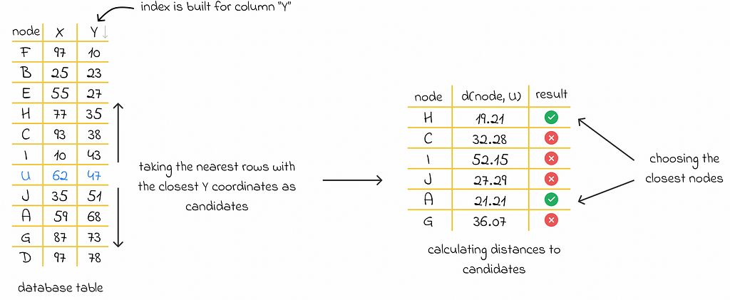
SQL databases allow the creation of an index — a data structure built on a certain column of a table accelerating the search process by keys in that column.
Another approach includes creating an index on one of the coordinate columns. When a user performs a query, the database can in O(1) time retrieve the position of the row in the table corresponding to the current position of the user.
Thanks to the constructed index, the database can also rapidly find the rows with the nearest coordinate value. Then it is possible to take a set of such rows and then filter those whose total Euclidean distance from the user position is less than a certain search radius.
Building an index on a column containing Y coordinates of nodes. As a consequence, it becomes very rapid to find a set of nodes whose Y coordinates are the nearest to a given node. However, the search process does not take into consideration any information about X coordinates, which is why the search results must be then filtered.
While the described approach is better than the previous one, it requires time to filter rows with the closest distances. Additionally, there can be cases when initially selected rows with the closest coordinates are not actually the closest ones to the user position.
A single table cannot have two indexes simultaneously. That is why for solving this problem, both coordinates should be represented as a single combined value while preserving information about distances. This objective is exactly achieved by quadtrees which are discussed in the next section.
Quadtree
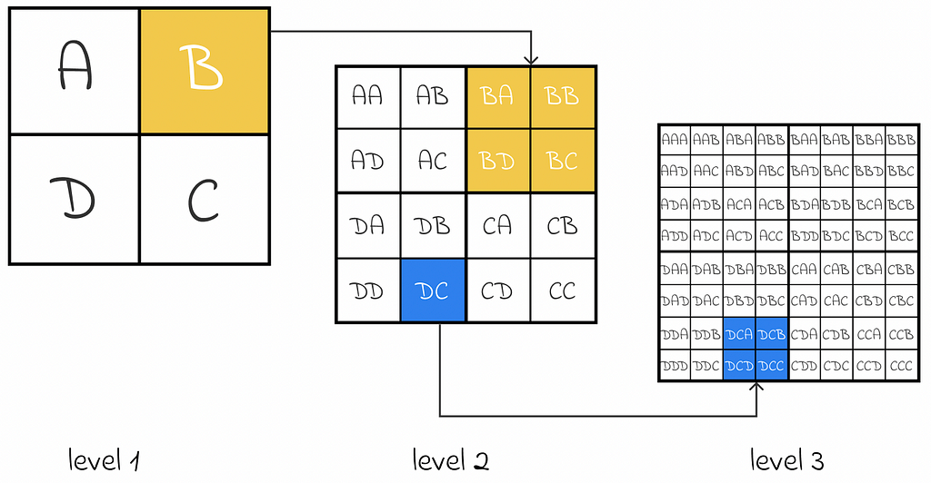
A quadtree is a tree data structure used for recursive partitioning of a 2D space into four quadrants. Depending on the tree structure, every parent node can have from 0 to 4 children.
Map representation in the quadtree format. The more levels are used, the higher the precision is.
As shown in the picture above, every square on a current level is divided by four equal subsquares in the next level. As a result, encoding a single square on level i requires 2 * i bits.
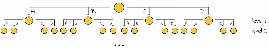
Quadtree visualisation
If a geographical map is divided in this way, then we can encode all of its subparts with a custom number of bits. The more levels are used in the quadtree, the better the precision is.
Properties
Quadtrees are particularly used in geo applications for several advantages:
Due to its structure, quadtrees allow rapid tree traversal.
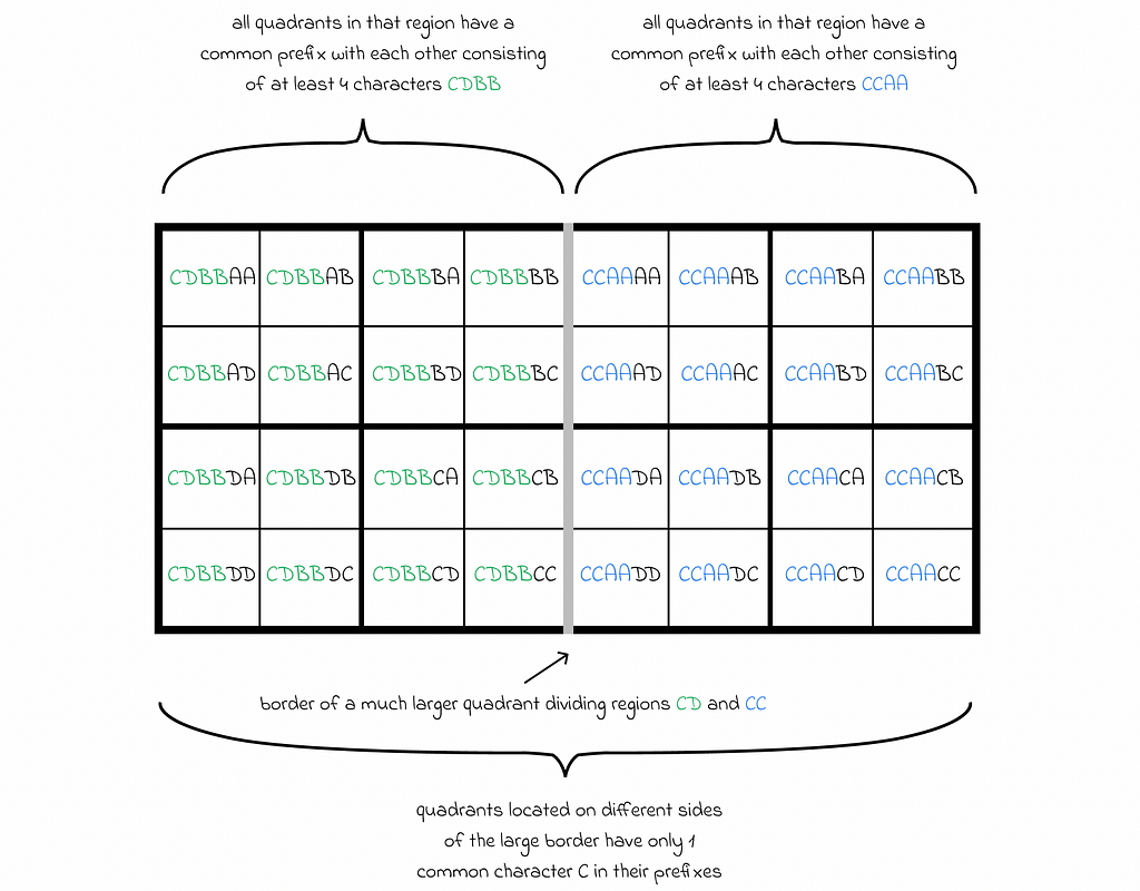
The larger the common prefix of two strings used to encode a pair of points on the map, the closer they are. However, this does not work the other way around in the edge case: a pair of points can be very close to each other but have a small common prefix. Though edge cases occur, they are not that often: they only happen when two small quadrants are located on opposite sides of a border with another much larger quadrant.
Edge case example: smaller quadrants on different sides of the border have only 1 common character in their prefixes
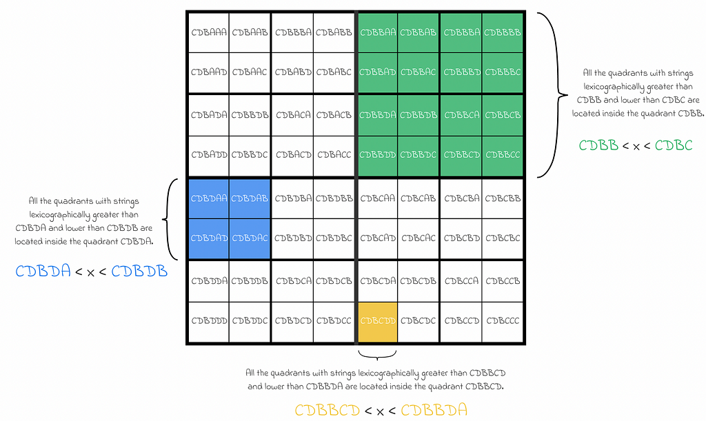
If a quadrant is represented by a string s₁s₂…sᵢ, then all of the subquadrants it contains, are represented by strings x such as s₁s₂…sᵢ < x < s₁s₂…sⱼ, where sⱼ is the next character after sᵢ in the lexicographical order.
Lexicographical order in quadtrees helps to rapidly identify all the subregions contained inside a larger region
Advantages
The main advantage of quadtrees is that every position on a map is represented by a unique string identifier which can be stored in a database as a single column making it possible to construct an index on quadtree strings. Therefore, given any string representing a region on the map, it becomes very fast:
to go up to higher levels or to move to lower levels of the region;
to access all the subregions of the region;
to find up to all of the 8 adjacent regions on the same level (except for edge cases).
GeoHash
In most real geographical applications, the GeoHash format is used which is a slight modification over the quadtree format:
instead of squares, geographical regions are divided by rectangles;
regions are divided into more than four parts;
every object on the map is encoded by a string in the “base 32” format consisting of digits 0–9 and lowercase letters except “a”, “i”, “l” and “o”.
Despite these slight modifications, GeoHash preserves the important advantages that were described in the section above for quadtrees.
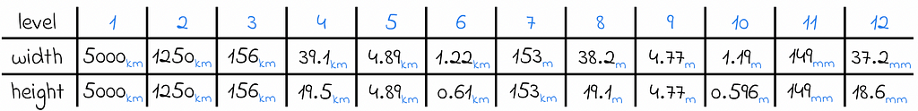
The table below shows the correspondance between every GeoHash level and rectangle sizes. For the large majority of cases, the levels 9 and 10 are already sufficient to give a very precise approximation on the map.
GeoHash correspondence between every encoding level and size of rectangles
Finding the nearest objects on the map
If we have on object on the map, we can find its nearest objects withing a certain distance d by using the following algorithm:
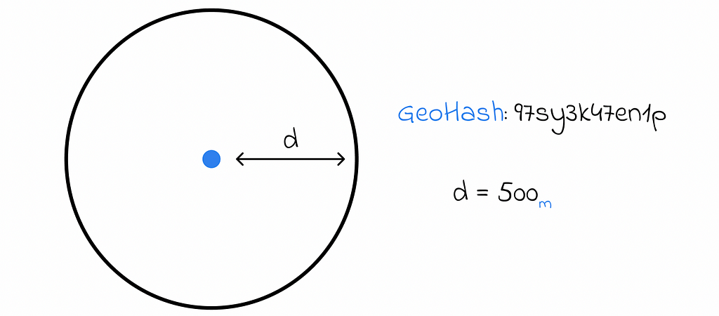
Converting the object to the GeoHash string s.
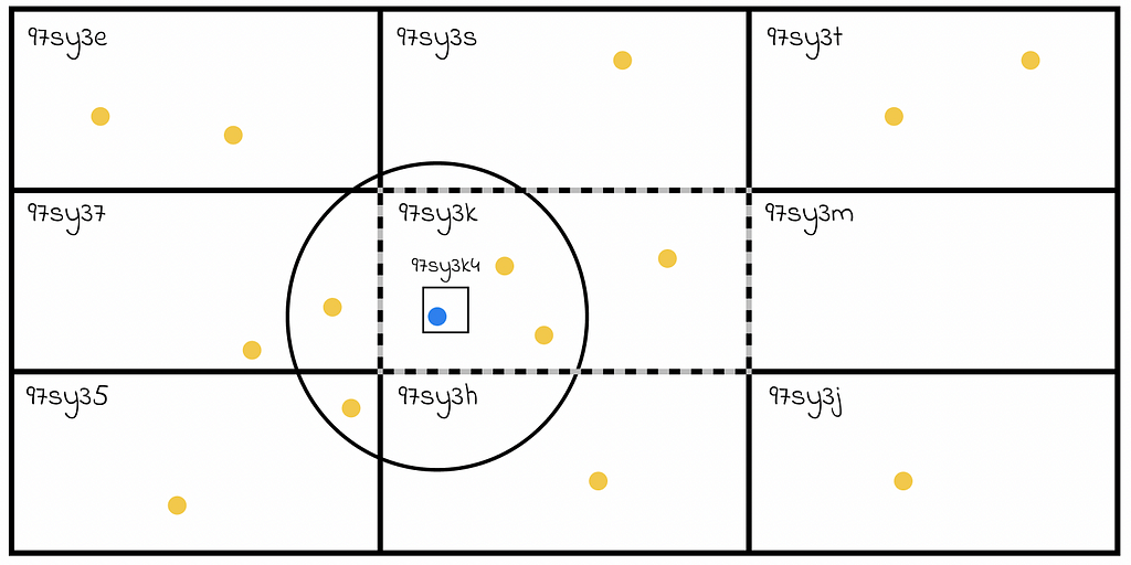
In this example, we would like to find all the objects located within d = 500 m from the blue node
2. Finding the first smallest GeoHash level i whose size is greater than the required distance d.
Level 6 is the first level whose width and height are greater than the search radius d
3. Take the first i characters of the string s (to represent the rectangle containing the initial object on level k).
4. Find 8 adjacent regions around the string s[0 … i – 1].
5. Find all the objects in the initial and adjacent regions and filter those objects whose distance to the initial object is less than d.
For the search process, all the objects inside the rectangle 97sy3k and its 8 adjacent rectangles must be considered. All the candidate objects are then linearly filtered to find those that satisfy the distance condition.
Conclusion
Fast navigation is a crucial aspect of geoapplications that use data about millions users and places. The key method for achiveing it includes the creation of a single index identifier that can implicitly represent both latitude and longitude.
By inheriting the most important properties of quadtrees, GeoHash server as a great example of such a method that indeed achieves great performance in practice. The only weak side of it is the presence of edge cases when both objects are located on different sides of a large border separating them. Though they might negatively affect the search efficiency, edge cases do not appear that often in practice meaning that GeoHash is still a top choice for geoapplications.
In case if you are familiar with machine learning and would like to learn more about optimized ways to perform scalable similarity search on embeddings, I recommend you go through my other series of articles on it:
Have you ever wondered how generative AI gets its work done? How does it create images, manage text, and perform other tasks?
The crucial concept you really need to understand is latent space. Understanding what the latent space is paves the way for comprehending generative AI.
Let me walk you through few examples to explain the essence of a latent space.
Example 1.Finding a better way to represent heights and weights data.
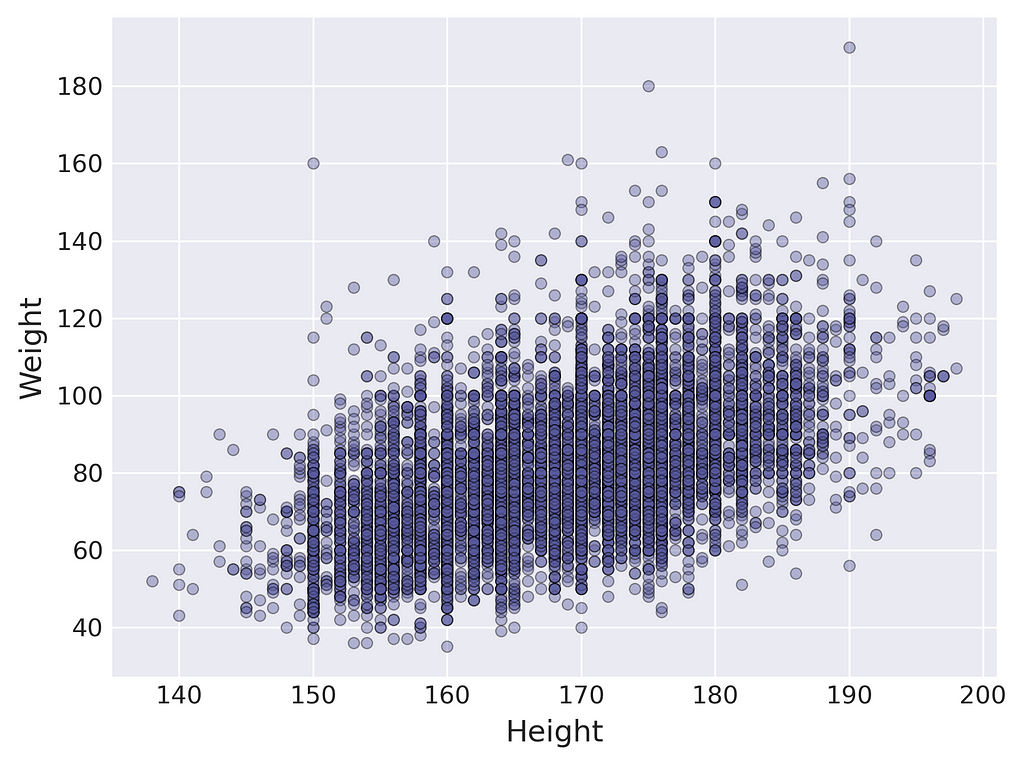
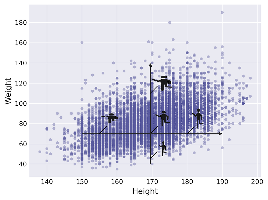
Throughout my numerous medical data research projects, I gathered a lot of measurements of patients’ weights and heights. The figure below shows the distribution of measurements.
Measurements of heights and weights of 11808 cardiac patients.
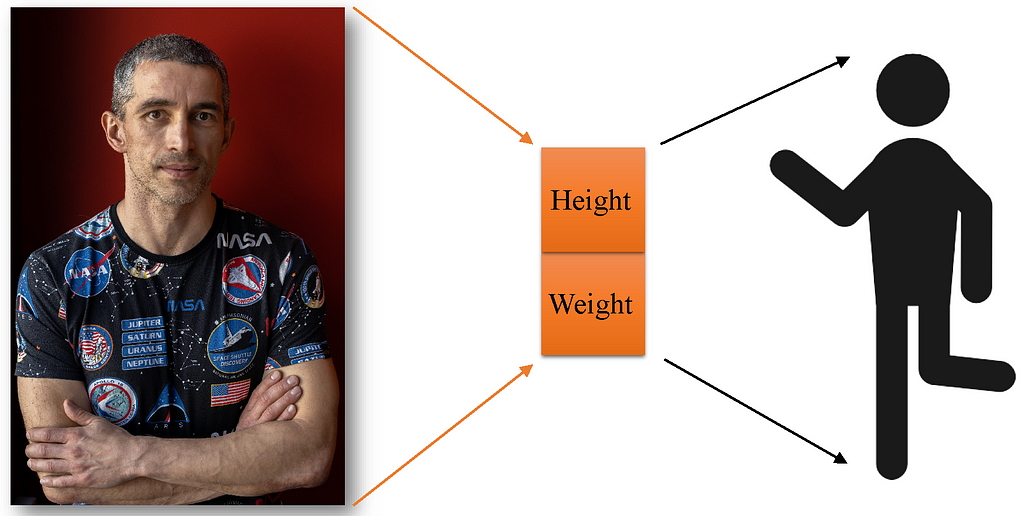
You can consider each point as a compressed version of information about a real person. All details such as facial features, hairstyle, skin tone, and gender are no longer available, leaving only weight and height values.
Is it possible to reconstruct the original data using only these two values? Sure, if your expectations aren’t too high. You simply need to replace all the discarded information with a standard template object to fill in the gaps. The template object is customized based on the preserved information, which in this case includes only height and weight.
Let’s delve into the space defined by the height and weight axes. Consider a point with coordinates of 170 cm for height and 70 kg for weight. Let this point serve as a reference figure and position it at the origin of the axes.
Moving horizontally keeps your weight constant while altering your height. Likewise, moving up and down keeps your height the same but changes your weight.
It might seem tricky because when you move in one direction, you have to think about two things simultaneously. Is there a way to improve this?
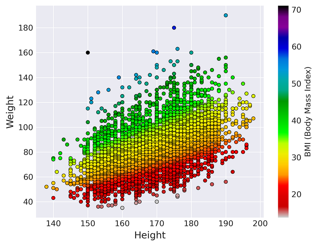
Take a look at the same dataset colour-coded by BMI.
The colors nearly align with the lines. This suggests that we could consider other axes that might be more convenient for generating human figures.
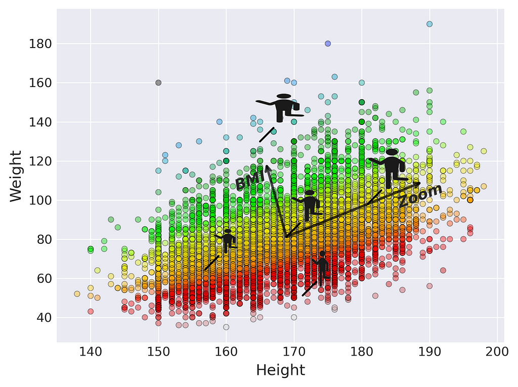
We might name one of these axes ‘Zoom’ because it maintains a constant BMI, with the only change being the scale of the figure. Likewise, the second axis could be labeled BMI.
The new axes offer a more convenient perspective on the data, making it easier to explore. You can specify a target BMI value and then simply adjust the size of the figure along the ‘Zoom’ axis.
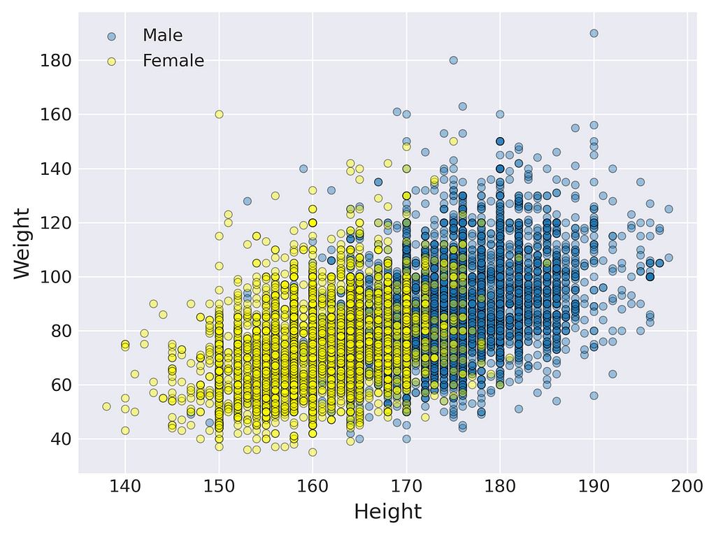
Looking to add more detail and realism to your figures? Consider additional features, such as gender, for instance. But from now on, I can’t offer similar visualizations that encompass all aspects of the data due to the lack of dimensions. I’m only able to display the distribution of three selected features: two features are depicted by the positions of points on the axes, with the third being indicated by color.
To improve the previous human figure generator, you can create separate templates for males and females. Then generate a female in yellow-dominant areas and a male where blue prevails.
As more features are taken into account, the figures become increasingly realistic. Notice also that a figure can be generated for every point, even those not present in the dataset.
This is what I would call a top-down approach to generate synthetic human figures. It involves selecting measurable features and identifying the optimal axes (directions) for exploring the data space. In the machine learning community, the first is called feature selection, and the second is termed feature extraction. Feature extraction can be carried out using specialized algorithms, e.g., PCA¹ (Principal Component Analysis), allowing the identification of directions that represent the data more naturally.
The mathematical space from which we generate synthetic objects is termed the latent space for two reasons. At first, the points (vectors) in this space are simply compressed, imperfect numerical representations of the original objects, much like shadows. Secondly, the axes defining the latent space often bear little resemblance to the originally measured features. The second reason will be better demonstrated in the next examples.
Example 2.Aging of human faces.
Twoday’s generative AI follows a bottom-up approach, where both feature selection and extraction are performed automatically from the raw data. Consider a vast dataset comprising images of faces, where the raw features consist of the colors of all pixels in each image, represented as numbers ranging from 0 to 255. A generative model like GAN² (Generative Adversarial Network) can identify (learn) a low-dimensional set of features where we can find the directions that interest us the most.
Imagine you want to develop an app that takes your image and shows you a younger or older version of yourself. To achieve this, you need to sort all latent space representations of images (latent space vectors) according to age. Then, for each age group, you have to determine the average vector.
If all goes well, the average vectors would align along a curve, which you can consider to approximate the age value axis.
Now, you can determine the latent space representation of your image (encoding step) and then move it along the age direction as you wish. Finally, you decode it to generate a synthetic image portraying the older (or younger) version of yourself. The idea of the decoding step here is similar to what I showed you in Example 1, but theoretically and computationally much more advanced.
The latent space allows exploration into other interesting dimensions, such as hair length, smile, gender, and more.
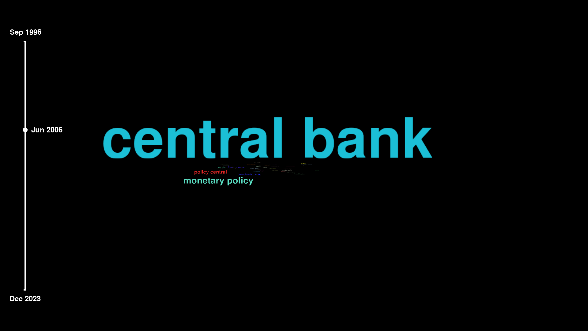
Example 3. Arranging words and phrases based on their meanings.
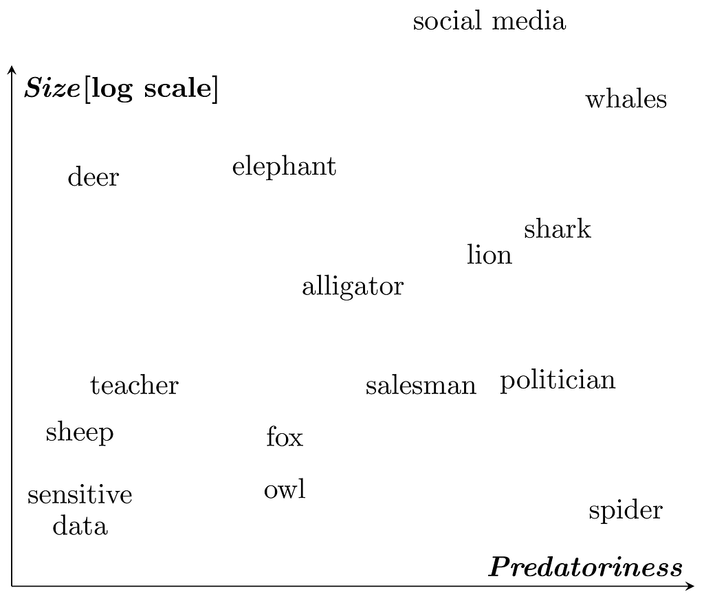
Let’s say you’re doing a study on predatory behavior in nature and society and you’ve got a ton of text material to analyze. For automating the filtering of relevant articles, you can encode words and phrases into the latent space. Following the top-down approach, let this latent space be based on two dimensions: Predatoriness and Size. In a real-world scenario, you’d need more dimensions. I only took two so you could see the latent space for yourself.
Below, you can see some words and phrases represented (embedded) in the introduced latent space. Using an analogy to physics: you can think of each word or phrase as being loaded with two types of charges: predatoriness and size. Words/phrases with similar charges are located close to each other in the latent space.
Every word/phrase is assigned numerical coordinates in the latent space.
These vectors are latent space representations of words/phrases and are referred to as embeddings. One of the great things about embeddings is that you can perform algebraic operations on them. For example, if you add the vectors representing ‘sheep’ and ‘spider’, you’ll end up close to the vector representing ‘politician’. This justifies the following elegant algebraic expression:
Do you think this equation makes sense?
Try out the latent space representation used by ChatGPT. This could be really entertaining.
Final words
The latent space represents data in a manner that highlights properties essential for the current task. Many AI methods, especially generative models and deep neural networks, operate on the latent space representation of data.
An AI model learns the latent space from data, projects the original data into this space (encoding step), performs operations within it, and finally reconstructs the result into the original data format (decoding step).
My intention was to help you understand the concept of the latent space. To delve deeper into the subject, I suggest exploring more mathematically advanced sources. If you have good mathematical skills, I recommend following the blog of Jakub Tomczak, where he discusses hot topics in the field of generative AI and offers thorough explanations of generative models.
Unless otherwise noted, all images are by the author.
What Is a Latent Space? was originally published in Towards Data Science on Medium, where people are continuing the conversation by highlighting and responding to this story.
We use cookies on our website to give you the most relevant experience by remembering your preferences and repeat visits. By clicking “Accept”, you consent to the use of ALL the cookies.
This website uses cookies to improve your experience while you navigate through the website. Out of these, the cookies that are categorized as necessary are stored on your browser as they are essential for the working of basic functionalities of the website. We also use third-party cookies that help us analyze and understand how you use this website. These cookies will be stored in your browser only with your consent. You also have the option to opt-out of these cookies. But opting out of some of these cookies may affect your browsing experience.
Necessary cookies are absolutely essential for the website to function properly. These cookies ensure basic functionalities and security features of the website, anonymously.
Cookie
Duration
Description
cookielawinfo-checkbox-analytics
11 months
This cookie is set by GDPR Cookie Consent plugin. The cookie is used to store the user consent for the cookies in the category "Analytics".
cookielawinfo-checkbox-functional
11 months
The cookie is set by GDPR cookie consent to record the user consent for the cookies in the category "Functional".
cookielawinfo-checkbox-necessary
11 months
This cookie is set by GDPR Cookie Consent plugin. The cookies is used to store the user consent for the cookies in the category "Necessary".
cookielawinfo-checkbox-others
11 months
This cookie is set by GDPR Cookie Consent plugin. The cookie is used to store the user consent for the cookies in the category "Other.
cookielawinfo-checkbox-performance
11 months
This cookie is set by GDPR Cookie Consent plugin. The cookie is used to store the user consent for the cookies in the category "Performance".
viewed_cookie_policy
11 months
The cookie is set by the GDPR Cookie Consent plugin and is used to store whether or not user has consented to the use of cookies. It does not store any personal data.
Functional cookies help to perform certain functionalities like sharing the content of the website on social media platforms, collect feedbacks, and other third-party features.
Performance cookies are used to understand and analyze the key performance indexes of the website which helps in delivering a better user experience for the visitors.
Analytical cookies are used to understand how visitors interact with the website. These cookies help provide information on metrics the number of visitors, bounce rate, traffic source, etc.
Advertisement cookies are used to provide visitors with relevant ads and marketing campaigns. These cookies track visitors across websites and collect information to provide customized ads.