Fine-tuning large language models (LLMs) creates tailored customer experiences that align with a brand’s unique voice. Amazon SageMaker Canvas and Amazon SageMaker JumpStart democratize this process, offering no-code solutions and pre-trained models that enable businesses to fine-tune LLMs without deep technical expertise, helping organizations move faster with fewer technical resources. SageMaker Canvas provides an intuitive […]
Phi-3 and the Beginning of Highly Performant iPhone LLMs
This blog post will go into the findings of the Phi-3 paper, as well as some of the implications of models like Phi-3 being released
Image by Author — generated by Stable Diffusion 2.1
Readers of my prior work may remember when I covered “Textbooks are all you need”, a paper by Microsoft showing how quality data can have an outsize impact on model performance. The findings there directly refuted the belief that models had to be enormous to be capable. The researchers behind that paper have continued their work and published something I find incredibly exciting.
Let’s dive into what the authors changed from the Phi-2 model, how they trained it, and how it works on your iPhone.
Key Terminology
There are a few key concepts to know before we dive into the architecture. If you know these already, feel free to skip to the next section.
A model’s parameters refer to the number of weights and biases that the model learns during training. If you have 1 billion parameters, then you have 1 billion weights and biases that determine the model’s performance. The more parameters you have the more complex your neural network can be. A head refers to the number of key, value, and query vectors the self-attention mechanism in a Transformer has. Layers refers to the number of neural segments that exist within the neural network of the Transformer, with hidden dimensions being the number of neurons within a typical hidden layer.
Tokenizer is the software piece that will convert your input text into an embedding that the transformer will then work with. Vocabulary size refers to the number of unique tokens that the model is trained on. The block structure of a transformer is how we refer to the combination of layers, heads, activation functions, tokenizer and layer normalizations that would be chosen for a specific model.
Grouped-Query Attention (GQA) is a way that we optimize multi-head attention to reduce the computational overhead during training and inference. As you can see from the image below, GQA takes the middle-ground approach — rather than pairing 1 value and 1 key to 1 query, we take a 1:1:M approach, with the many being smaller than the entire body of queries. This is done to still get the training cost benefits from Multi-Query Attention (MQA), while minimizing the performance degradation that we see follow that.
Phi 3 Architecture
Let’s begin with the architecture behind this model. The researchers released 3 different decoder only models, phi-3-mini, phi-3-small, and phi-3-medium, with different hyperparameters for each.
Going into some of the differences here, the phi-3-mini model was trained using typical mutli-head attention. While not called out in the paper, my suspicion is that because the model is roughly half the size of the other two, the training costs associated with multi-head were not objectionable. Naturally when they scaled up for phi-3-small, they went with grouped query attention, with 4 queries connected to 1 key.
Moreover, they kept phi-3-mini’s block structure as close to the LLaMa-2 structure as they could. The goal here was to allow the open-source community to continue their research on LLaMa-2 with Phi-3. This makes sense as a way to further understand the power of that block structure.
However, phi-3-small did NOT use LLaMa’s block structure, opting to use the tiktoken tokenizer, with alternate layers of dense attention and a new blocksparse attention. Additionally, they added in 10% multilingual data to the training dataset for these models.
Training and Data Optimal Mixes
Similar to Phi-2, the researchers invested majorly in quality data. They used the similar “educational value” paradigm they had used before when generating data to train the model on, opting to use significantly more data than last time. They created their data in 2 phases.
Phase-1 involved finding web data that they found was of high “educational value” to the user. The goal here is to give general knowledge to the model. Phase-2 then takes a subset of the Phase-1 data and generates data that would teach the model how to logically reason or attain specific skills.
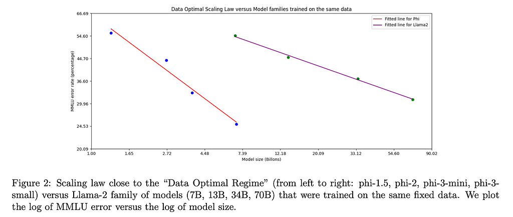
The challenge here was to ensure the mix of data from each corpus was appropriate for the scale of the model being trained (ie phi-3-small vs phi-3-mini). This is the idea behind a “data optimal” regime, where the data you are giving to the LLM to train with gives it the best ability for its block structure. Put differently, if you think that data is a key distinguisher for training a good LLM, then finding the right combination of skills to show the model via your data can be just as key as finding good data. The researchers highlighted that they wanted the model to have stronger reasoning than knowledge abilities, resulting in their choosing more data from the Phase-2 corpus than from the Phase-1.
Figure 2 from the paper highlighting a potential relationship for data optimality
Interestingly, when they were training phi-3-medium with roughly the same data mixture as they trained phi-3-small, they noticed that the improvements from 7B parameters to 14B were far more limited than from 3.8B to 7B. The authors suspect this is not a limitation of the block structure, but instead of the data mixture they used to train phi-3-medium.
Post-Training
The team used both Supervised Fine Tuning (SFT) and Direct Preference Optimization (DPO) to improve the model post-training. Those interested in a deep dive on DPO can check out my blog post here. Supervised Fine Tuning is a type of transfer learning where we use a custom dataset to improve the LLM’s capabilities on that dataset. The authors used SFT to improve the model’s ability across diverse domains like math, coding, reasoning, and safety. They then used DPO for their chat optimization to guide it away from responses they wanted to avoid and towards ideal responses.
It’s in this stage that the authors expanded the context window of phi-3-mini from 4k tokens to 128k tokens. The methodology they used to do this is called Long Rope. The authors claim that the performance is consistent between the 2 context types, which is a big deal given the enormous increase in context length. If there is sufficient interest, I will do a separate blog post on the findings within that paper.
Quantization for Phone Usage
Even though these models are small, to get these models to run on your phone still requires some further minimization. Typically the weights for a LLM is stored as float; for example, Phi-3’s original weights were bfloat16, meaning each weight takes up 16 bits in memory. While 16 bits may seem trivial, when you take into account there are on the order of 10⁹ parameters in the model, you realize how quickly each additional bit adds up.
To get around this, the authors condensed the weights from 16 bits to 4 bits. The basic idea is to reduce the number of bits required to store each number. For a conceptual example, the number 2.71828 could be condensed to 2.72. While this is a lossy operation, it still captures a good portion of the information while taking significantly less storage.
The authors ran the quantized piece on an iPhone with the A16 chip and found it could generate up to 12 tokens per second. For comparison, an M1 MacBook running LLaMa-2 Quantized 4 bit runs at roughly 107 tokens per second. The fastest token generation I’ve seen (Groq) generated tokens at a rate of 853.35 Tokens per second. Given this is just the beginning, it’s remarkable how fast we are able to see tokens generated on an iPhone with this model. It seems likely the speed of inference will only increase.
Pairing Phi-3 with Search
One limitation with a small model is it has fewer places it can store information within its network. As a result, we see that Phi-3 does not perform as well as models like LLaMa-2 on tasks that require wide scopes of knowledge.
The authors suggest that by pairing Phi-3 with a search engine the model’s abilities will significantly improve. If this is the case, that makes me think Retrieval Augmented Generation (RAG) is likely here to stay, becoming a critical part of helping small models be just as performant as larger ones.
Figure 4 from the paper highlighting how search can improve Phi-3 performance
Conclusion
In closing, we are seeing the beginning of highly performant smaller models. While training these models still relies to a large degree on performant hardware, inferencing them is increasingly becoming democratized. This introduces a few interesting phenomena.
First, models that can run locally can be almost fully private, allowing users to give these LLMs data that they otherwise may not feel comfortable sending over the internet. This opens the door to more use cases.
Second, these models will drive mobile hardware to be even more performant. As a consequence, I would expect to see more Systems on Chips (SoC) on high-end smartphones, especially SoCs with shared memory between CPUs and GPUs to maximize the speed of inference. Moreover, the importance of having quality interfaces with this hardware will be paramount. Libraries like MLX for Apple Silicon will likely be required for any new hardware entrants in the consumer hardware space.
Third, as this paper shows that high quality data can in many ways outcompete more network complexity in an LLM, the race to not just find but generate high quality data will only increase.
Feature selection is a critical step in many machine learning pipelines. In practice, we generally have a wide range of variables available as predictors for our models, but only a few of them are related to our target. Feature selection consists of finding a reduced set of these features, mainly for:
Improved generalization — using a reduced number of features minimizes the risk of overfitting.
Better inference — by removing redundant features (for example, two features very correlated with each other), we can retain only one of them and better capture its effect.
Efficient training — having less features means shorter training times.
Better interpretation — reducing the number of features produces more parsimonious models which are easier to understand.
There are many techniques available to perform feature selection, each with varying complexity. In this article, I want to share a way of using a powerful open source optimization tool, Optuna, to perform the feature selection task in an innovative way. The main idea is to have a flexible tool that can handle feature selection for a wide range of tasks, by efficiently testing different feature combinations (e.g., not trying them all one by one). Below, we’ll go through a hands-on example implementing this approach, and also comparing it to other common feature selection strategies. To experiment with the feature selection techniques discussed, you can follow along with this Colab Notebook.
In this example, we’ll focus on a classification task based on the Mobile Price Classification dataset from Kaggle. We have 20 features, including ‘battery_power’, ‘clock_speed’ and ‘ram’, to predict the ‘price_range’ feature, which can belong to four different bands: 0, 1, 2 and 3.
We first split our dataset into train and test sets, and we also prepare a 5-fold validation split within the train set — this will be useful later on.
import pandas as pd from sklearn.model_selection import train_test_split from sklearn.model_selection import StratifiedKFold
SEED = 32
# Load data filename = "train.csv" # train.csv from https://www.kaggle.com/datasets/iabhishekofficial/mobile-price-classification
# The last column is the target variable X_train = df_train.iloc[:,0:20] y_train = df_train.iloc[:,-1] X_test = df_test.iloc[:,0:20] y_test = df_test.iloc[:,-1]
# Stratified kfold over the train set for cross validation skf = StratifiedKFold(n_splits=5, shuffle=True, random_state=SEED) splits = list(skf.split(X_train, y_train))
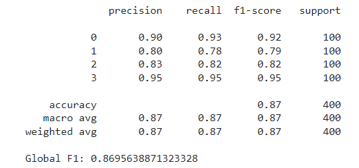
The model we’ll use throughout the example is the Random Forest Classifier, using the scikit-learn implementation and default parameters. We first train the model using all features to set our benchmark. The metric we’ll measure is the F1 score weighted for all four price ranges. After fitting the model over the train set, we evaluate it on the test set, obtaining an F1 score of around 0.87.
from sklearn.ensemble import RandomForestClassifier from sklearn.metrics import f1_score, classification_report
model = RandomForestClassifier(random_state=SEED) model.fit(X_train,y_train) preds = model.predict(X_test)
The goal now is to improve these metrics by selecting a reduced feature set. We will first outline how our Optuna-based approach works, and then test and compare it with other common feature selection strategies.
Optuna
Optuna is an optimization framework mainly used for hyperparameter tuning. One of the key features of the framework is its use of Bayesian optimization techniques to search the parameter space. The main idea is that Optuna tries different combinations of parameters and evaluates how the objective function changes with each configuration. From these trials, it builds a probabilistic model used to estimate which parameter values are likely to yield better outcomes.
This strategy is much more efficient compared to grid or random search. For example, if we had n features, and attempted to try each possible feature subset, we would have to perform 2^n trials. With 20 features these would be more than a million trials. Instead, with Optuna, we can explore the search space with much fewer trials.
Optuna offers various samplers to try. For our case, we’ll use the default one, the TPESampler, based on the Tree-structured Parzen Estimator algorithm (TPE). This sampler is the most commonly used, and it’s recommended for searching categorical parameters, which is our case as we’ll see below. According to the documentation, this algorithm “fits one Gaussian Mixture Model (GMM) l(x) to the set of parameter values associated with the best objective values, and another GMM g(x) to the remaining parameter values. It chooses the parameter value x that maximizes the ratio l(x)/g(x).”
As mentioned earlier, Optuna is typically used for hyperparameter tuning. This is usually done by training the model repeatedly on the same data using a fixed set of features, and in each trial testing a new set of hyperparameters determined by the sampler. The parameter set that minimizes the given objective function is then returned as the best trial.
In our case, however, we’ll use a fixed model with predetermined parameters, and in each trial, we’ll allow Optuna to select which features to try. The process aims to find the set of features that minimizes the loss function. In our case, we’ll guide the algorithm to maximize the F1 score (or minimize the negative of the F1). Additionally, we’ll add a small penalty for each feature used, to encourage smaller feature sets (if two feature sets yield similar results, we’ll prefer the one with fewer features).
The data we’ll use is the train dataset, split into five folds. In each trial, we’ll fit the classifier five times using four of the five folds for training and the remaining fold for validation. We’ll then average the validation metrics and add the penalty term to calculate the trial’s loss.
Below is the implemented class to perform the feature selection search:
import optuna
class FeatureSelectionOptuna: """ This class implements feature selection using Optuna optimization framework.
Parameters:
- model (object): The predictive model to evaluate; this should be any object that implements fit() and predict() methods. - loss_fn (function): The loss function to use for evaluating the model performance. This function should take the true labels and the predictions as inputs and return a loss value. - features (list of str): A list containing the names of all possible features that can be selected for the model. - X (DataFrame): The complete set of feature data (pandas DataFrame) from which subsets will be selected for training the model. - y (Series): The target variable associated with the X data (pandas Series). - splits (list of tuples): A list of tuples where each tuple contains two elements, the train indices and the validation indices. - penalty (float, optional): A factor used to penalize the objective function based on the number of features used. """
def __init__(self, model, loss_fn, features, X, y, splits, penalty=0):
self.model = model self.loss_fn = loss_fn self.features = features self.X = X self.y = y self.splits = splits self.penalty = penalty
def __call__(self, trial: optuna.trial.Trial):
# Select True / False for each feature selected_features = [trial.suggest_categorical(name, [True, False]) for name in self.features]
# List with names of selected features selected_feature_names = [name for name, selected in zip(self.features, selected_features) if selected]
# Optional: adds a penalty for the amount of features used n_used = len(selected_feature_names) total_penalty = n_used * self.penalty
loss = 0
for split in self.splits: train_idx = split[0] valid_idx = split[1]
# Train model, get predictions and accumulate loss self.model.fit(X_train_selected, y_train) pred = self.model.predict(X_valid_selected)
loss += self.loss_fn(y_valid, pred)
# Take the average loss across all splits loss /= len(self.splits)
# Add the penalty to the loss loss += total_penalty
return loss
The key part is where we define which features to use. We treat each feature as one parameter, which can take the values True or False. These values indicate whether the feature should be included in the model. We use the suggest_categorical method so that Optuna selects one of the two possible values for each feature.
We now initialize our Optuna study and perform the search for 100 trials. Notice that we enqueue a first trial using all features, as a starting point for the search, allowing Optuna to compare subsequent trials against a fully-featured model:
from optuna.samplers import TPESampler
def loss_fn(y_true, y_pred): """ Returns the negative F1 score, to be treated as a loss function. """ res = -f1_score(y_true, y_pred, average='weighted') return res
features = list(X_train.columns)
model = RandomForestClassifier(random_state=SEED)
sampler = TPESampler(seed = SEED) study = optuna.create_study(direction="minimize",sampler=sampler)
# We first try the model using all features default_features = {ft: True for ft in features} study.enqueue_trial(default_features)
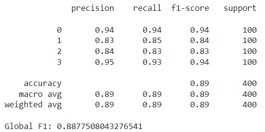
Notice that from the original 20 features, the search concluded with only 9 of them, which is a significant reduction. These features yielded a minimum validation loss of around -0.9117, which means they achieved an average F1 score of around 0.9108 across all folds (after adjusting for the penalty term).
The next step is to train the model on the entire train set using these selected features and evaluate it on the test set. This results in an F1 score of around 0.882:
Image by author
By selecting the right features, we were able to reduce our feature set by more than half, while still achieving a higher F1 score than with the full set. Below we will discuss some pros and cons of using Optuna for feature selection:
Pros:
Searches across feature sets efficiently, taking into account which feature combinations are most likely to produce good results.
Adaptable for many scenarios: As long as there is a model and a loss function, we can use it for any feature selection task.
Sees the whole picture: Unlike methods that evaluate features individually, Optuna takes into account which features tend to go well with each other, and which don’t.
Dynamically determines the number of features as part of the optimization process. This can be tuned with the penalty term.
Cons:
It’s not as straightforward as simpler methods, and for smaller and simpler datasets it might not be worth it.
Although it requires much fewer trials than other methods (like exhaustive search), it still typically requires around 100 to 1000 trials. Depending on the model and dataset, this can be time-consuming and computationally expensive.
Next, we’ll compare our approach to other common feature selection strategies.
Other Methods
Filter Methods — Chi-Squared
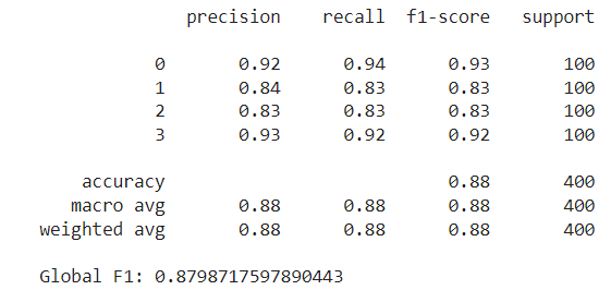
One of the simplest alternatives is to evaluate each feature individually using a statistial test and retain the top k features based on their scores. Notice that this approach doesn’t require any machine learning model. For example, for the classification task, we can choose the chi-squared test, which determines whether there is a statistically significant association between each feature and the target variable. We’ll use the SelectKBest class from scikit-learn, which applies the score function (chi-squared) to each feature and returns the top k scoring variables. Unlike the Optuna method, the number of features isn’t determined in the selection process, but must be set beforehand. In this case, we’ll set this number at ten. These methods fall within the filter methods class. They tend to be the easiest and fastest to compute since they don’t require any model behind.
from sklearn.feature_selection import SelectKBest, chi2
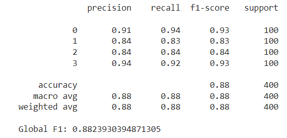
In our case, ram scored the highest by far in the chi-squared test, followed by px_height and battery_power. Notice that these features were also selected by our Optuna method above, along with px_width, mobile_wt and sc_w. However, there are some new additions like int_memory and talk_time — these weren’t picked by the Optuna study. After training the random forest with these 10 features and evaluating it on the test set, we achieved an F1 score slightly higher than our previous best, at approximately 0.888:
Image by author
Pros:
Model agnostic: doesn’t require a machine learning model.
Easy and fast to implement and run.
Cons:
It has to be adapted for each task. For instance, some score functions are only applicable for classification tasks, and others only for regression tasks.
Greedy: depending on the alternative used, it usually looks at features one by one, without taking into account which are already included in the set.
Requires the number of features to select to be set beforehand.
Wrapper Methods — Forward Search
Wrapper methods are another class of feature selection strategies. These are iterative methods; they involve training the model with a set of features, evaluating its performance, and then deciding whether to add or remove features. Our Optuna strategy falls within these methods. However, most common examples include forward selection or backward selection. With forward selection, we begin with no features and, at each step, we greedily add the feature that provides the highest performance gain, until a stop criterion is met (number of features or performance decline). Conversely, backward selection starts with all features and iteratively removes the least significant ones at each step.
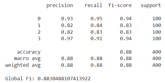
Below, we try the SequentialFeatureSelector class from scikit-learn, performing a forward selection until we find the top 10 features. This method will also make use of the 5-fold split we performed above, averaging performance across the validation splits at each step.
from sklearn.feature_selection import SequentialFeatureSelector
model = RandomForestClassifier(random_state=SEED) sfs = SequentialFeatureSelector(model, n_features_to_select=10, cv=splits) sfs.fit(X_train, y_train);
Again, some are common to the previous methods, and some are new (e.g., three_g and touch_screen. Using these features, the Random Forest achieves a lower test F1 score, slightly below 0.88.
Image by author
Pros
Easy to implement in just a few lines of code.
It can also be used to determine the number of features to use (using the tolerance parameter).
Cons
Time consuming: Starting with zero features, it trains the model each time using a different variable, and retains the best one. For the next step, it again tries out all features (now including the previous one), and again selects the best one. This is repeated until the desired number of features is reached.
Greedy: Once a feature is included, it stays. This may lead to suboptimal results, as the feature providing the highest individual gain in early rounds might not be the best choice in the context of other feature interactions.
Feature Importance
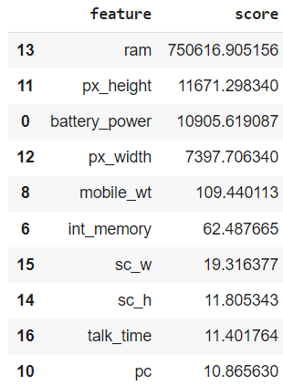
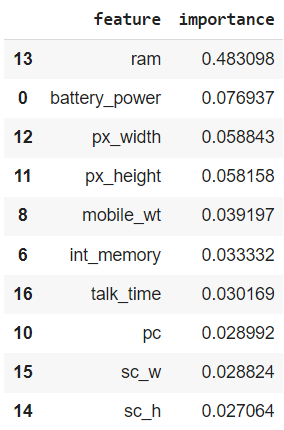
Finally, we’ll explore another straightforward selection strategy, which involves using the feature importances the model learns (if available). Certain models, like Random Forests, provide a measure of which features are most important for prediction. We can use these rankings to filter out those features that, according to the model, have the least importance. In this case, we train the model on the entire train dataset, and retain the 10 most important features:
model = RandomForestClassifier(random_state=SEED) model.fit(X_train,y_train)
Notice how, once again, ram is ranked highest, far above the second most important feature. Training with these 10 features, we obtain a test F1 score of almost 0.883, similar to the ones we’ve been seeing. Also, note how the features selected through feature importance are the same as those selected using the chi-squared test, although they are ranked differently. This difference in ranking results in a slightly different outcome.
Image by author
Pros:
Easy and fast to implement: it requires a single training of the model and directly uses the derived feature importances.
It can be adapted into a recursive version, in which at each step the least important feature is removed and the model is then trained again (see Recursive Feature Elimination).
Contained within the model: If the model we are using provides feature importances, we already have a feature selection alternative available at no additional cost.
Cons:
Feature importance might not be aligned with our end goal. For instance, a feature might appear unimportant on its own but could be critical due to its interaction with other features. Also, an important feature might be counterproductive overall, by affecting the performance of other useful predictors.
Not all models offer feature importance estimation.
Requires the number of features to select to be predefined.
Closing Remarks
To conclude, we’ve seen how to use Optuna, a powerful optimization tool, for the feature selection task. By efficiently navigating the search space, it is able to find good feature subsets with relatively few trials. Not only that, but it is also flexible and can be adapted to many scenarios as long as we have a model and a loss function defined.
Throughout our examples, we observed that all techniques yielded similar feature sets and results. This is mainly because the dataset we used is rather simple. In these cases, simpler methods already produce a good feature selection, so it wouldn’t make much sense to go with the Optuna approach. However, for more complex datasets, with more features and intricate relationships between them, using Optuna might be a good idea. So, all in all, given its relative ease of implementation and ability to deliver good results, using Optuna for feature selection is a worthwhile addition to the data scientist’s toolkit.
Not so long ago, it seemed like landing your first data science job or switching to a more exciting data or ML role followed a fairly well-defined sequence. You learned new skills and expanded your existing ones, demonstrated your experience, zoomed in on the most fitting listings, and… sooner or later, something good would come your way.
Of course, things were never quite as straightforward, at least not for everyone. But even so, we’ve experienced somewhat of a mood shift in the past few months: the job market is more competitive, companies’ hiring processes more demanding, and there appears to be a lot more uncertainty and fluidity in tech and beyond.
What is an ambitious data professional to do? We prefer to avoid shortcuts and magic hacks in favor of foundational skills that showcase your deep understanding of the problems you aim to solve. Our most seasoned authors seem to point at the same direction: the lineup of articles we’re highlighting this week offer concrete insights for data and ML practitioners across a wide span of career stages and focus areas; they foreground continuous learning and building resilience in the face of change. Enjoy your reading!
One Mindset Shift That Will Make You a Better Data Scientist “I’ve grown convinced that an ownership mentality is one of the key things that sets high performers apart from their peers.” Tessa Xie reflects on her own data science journey and outlines the three most common manifestations of this type of proactive mindset—and how to grow towards it step by step.
A New Manager’s Guide to High Performing Data Science Teams If you’ve finally achieved your goal to step into a management role, you might quickly discover that a whole new set of challenges awaits you. Zachary Raicik offers thoughtful advice on how to start on the right foot and set yourself—and your team—up for long-term success.
Combining Storytelling and Design for Unforgettable Presentations Regardless of role, seniority level, or project type, effective storytelling remains one of the most crucial skills data professionals can develop to ensure their work reaches its audience and makes an impact. Hennie de Harder offers actionable guidelines for crafting a compelling slide deck that packs a punch and delivers your message to diverse audiences of stakeholders.
How to Keep on Developing as a Data Scientist For Eryk Lewinson, “being a data scientist often involves having the mentality of a lifelong learner.” While courses, books, and other resources abound, what makes his advice particularly helpful is its focus on learning that can take place during your regular work hours, from pair programming and mentoring to knowledge exchanges and feedback cycles.
There are so many different ways to grow as data and machine learning professionals; our other reading recommendations this week can each be its own point of departure for learning about new skills, tools, and workflows.
Thank you for supporting the work of our authors! We love publishing articles from new authors, so if you’ve recently written an interesting project walkthrough, tutorial, or theoretical reflection on any of our core topics, don’t hesitate to share it with us.
We use cookies on our website to give you the most relevant experience by remembering your preferences and repeat visits. By clicking “Accept”, you consent to the use of ALL the cookies.
This website uses cookies to improve your experience while you navigate through the website. Out of these, the cookies that are categorized as necessary are stored on your browser as they are essential for the working of basic functionalities of the website. We also use third-party cookies that help us analyze and understand how you use this website. These cookies will be stored in your browser only with your consent. You also have the option to opt-out of these cookies. But opting out of some of these cookies may affect your browsing experience.
Necessary cookies are absolutely essential for the website to function properly. These cookies ensure basic functionalities and security features of the website, anonymously.
Cookie
Duration
Description
cookielawinfo-checkbox-analytics
11 months
This cookie is set by GDPR Cookie Consent plugin. The cookie is used to store the user consent for the cookies in the category "Analytics".
cookielawinfo-checkbox-functional
11 months
The cookie is set by GDPR cookie consent to record the user consent for the cookies in the category "Functional".
cookielawinfo-checkbox-necessary
11 months
This cookie is set by GDPR Cookie Consent plugin. The cookies is used to store the user consent for the cookies in the category "Necessary".
cookielawinfo-checkbox-others
11 months
This cookie is set by GDPR Cookie Consent plugin. The cookie is used to store the user consent for the cookies in the category "Other.
cookielawinfo-checkbox-performance
11 months
This cookie is set by GDPR Cookie Consent plugin. The cookie is used to store the user consent for the cookies in the category "Performance".
viewed_cookie_policy
11 months
The cookie is set by the GDPR Cookie Consent plugin and is used to store whether or not user has consented to the use of cookies. It does not store any personal data.
Functional cookies help to perform certain functionalities like sharing the content of the website on social media platforms, collect feedbacks, and other third-party features.
Performance cookies are used to understand and analyze the key performance indexes of the website which helps in delivering a better user experience for the visitors.
Analytical cookies are used to understand how visitors interact with the website. These cookies help provide information on metrics the number of visitors, bounce rate, traffic source, etc.
Advertisement cookies are used to provide visitors with relevant ads and marketing campaigns. These cookies track visitors across websites and collect information to provide customized ads.