Tag: AI

Develop and deploy an entirely local RAG system from scratch

Introduction

High-level abstractions offered by libraries like llama-index and Langchain have simplified the development of Retrieval Augmented Generation (RAG) systems. Yet, a deep understanding of the underlying mechanics enabling these libraries remains crucial for any machine learning engineer aiming to fully leverage their potential. In this article, I will guide you through the process of developing a RAG system from the ground up. I will also take it a step further, and we will create a containerized flask API. I have designed this to be highly practical: this walkthrough is inspired by real-life use cases, ensuring that the insights you gain are not only theoretical but immediately applicable.

Use-case overview — This implementation is designed to handle a wide array of document types. While the current example utilizes many small documents, each depicting individual products with details such as SKU, name, description, price, and dimensions, the approach is highly adaptable. Whether the task involves indexing a diverse library of books, mining data from extensive contracts, or any other set of documents, the system can be tailored to meet the specific needs of these varied contexts. This flexibility allows for the seamless integration and processing of different types of information.

Quick note — this implementation will work solely with text data. Similar steps can be followed to convert images to embeddings using a multi-modal model like CLIP, which you can then index and query against.

Table of Contents

• Outline the modular framework
• Prepare the data
• Chunking, indexing, and retrieval (core functionality)
• LLM component
• Build and deploy the API
• Conclusion

Modular Framework

The implementation has four main components that can be swapped out.

• Text data
• Embedding model
• LLM
• Vector store

Integrating these services into your project is highly flexible, allowing you to tailor them according to your specific requirements. In this example implementation, I start with a scenario where the initial data is in a JSON format, which conveniently provides the data as a string. However, you might encounter data in various other formats such as PDFs, emails, or Excel spreadsheets. In such cases, it is essential to “normalize” this data by converting it into a string format. Depending on the needs of your project, you can either convert the data to a string in memory or save it to a text file for further refinement or downstream processing.

Similarly, the choices of embeddings model, vector store, and LLM can be customized to fit your project’s needs. Whether you require a smaller or larger model, or perhaps an external model, the flexibility of this approach allows you to simply swap in the appropriate options. This plug-and-play capability ensures that your project can adapt to various requirements without significant alterations to the core architecture.

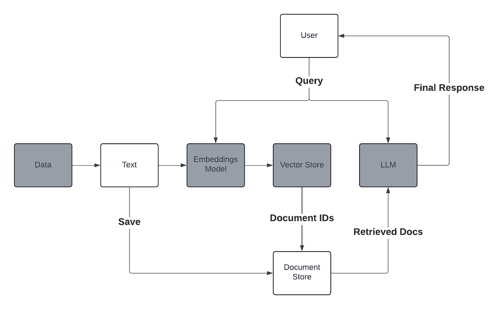
I highlighted the main components in gray. In this implementation our vector store will simply be a JSON file. Once again, depending on your use-case, you may want to just use an in-memory vector store (Python dict) if you’re only processing one file at a time. If you need to persist this data, like we do for this use-case, you can save it to a JSON file locally. If you need to store hundreds of thousands or millions of vectors you would need an external vector store (Pinecone, Azure Cognitive Search, etc…).

Prepare Data

As mentioned above, this implementation starts with JSON data. I used GPT-4 and Claude to generate it synthetically. The data contains product descriptions for different pieces of furniture each with its own SKU. Here is an example:

{
    "MBR-2001": "Traditional sleigh bed crafted in rich walnut wood, featuring a curved headboard and footboard with intricate grain details. Queen size, includes a plush, supportive mattress. Produced by Heritage Bed Co. Dimensions: 65"W x 85"L x 50"H.",
    "MBR-2002": "Art Deco-inspired vanity table in a polished ebony finish, featuring a tri-fold mirror and five drawers with crystal knobs. Includes a matching stool upholstered in silver velvet. Made by Luxe Interiors. Vanity dimensions: 48"W x 20"D x 30"H, Stool dimensions: 22"W x 16"D x 18"H.",
    "MBR-2003": "Set of sheer linen drapes in soft ivory, offering a delicate and airy touch to bedroom windows. Each panel measures 54"W x 84"L. Features hidden tabs for easy hanging. Manufactured by Tranquil Home Textiles.",

    "LVR-3001": "Convertible sofa bed upholstered in navy blue linen fabric, easily transitions from sofa to full-size sleeper. Perfect for guests or small living spaces. Features a sturdy wooden frame. Produced by SofaBed Solutions. Dimensions: 70"W x 38"D x 35"H.",
    "LVR-3002": "Ornate Persian area rug in deep red and gold, hand-knotted from silk and wool. Adds a luxurious touch to any living room. Measures 8' x 10'. Manufactured by Ancient Weaves.",
    "LVR-3003": "Contemporary TV stand in matte black with tempered glass doors and chrome legs. Features integrated cable management and adjustable shelves. Accommodates up to 65-inch TVs. Made by Streamline Tech. Dimensions: 60"W x 20"D x 24"H.",

    "OPT-4001": "Modular outdoor sofa set in espresso brown polyethylene wicker, includes three corner pieces and two armless chairs with water-resistant cushions in cream. Configurable to fit any patio space. Produced by Outdoor Living. Corner dimensions: 32"W x 32"D x 28"H, Armless dimensions: 28"W x 32"D x 28"H.",
    "OPT-4002": "Cantilever umbrella in sunflower yellow, featuring a 10-foot canopy and adjustable tilt for optimal shade. Constructed with a sturdy aluminum pole and fade-resistant fabric. Manufactured by Shade Masters. Dimensions: 120"W x 120"D x 96"H.",
    "OPT-4003": "Rustic fire pit table made from faux stone, includes a natural gas hookup and a matching cover. Ideal for evening gatherings on the patio. Manufactured by Warmth Outdoor. Dimensions: 42"W x 42"D x 24"H.",

    "ENT-5001": "Digital jukebox with touchscreen interface and built-in speakers, capable of streaming music and playing CDs. Retro design with modern technology, includes customizable LED lighting. Produced by RetroSound. Dimensions: 24"W x 15"D x 48"H.",
    "ENT-5002": "Gaming console storage unit in sleek black, featuring designated compartments for systems, controllers, and games. Ventilated to prevent overheating. Manufactured by GameHub. Dimensions: 42"W x 16"D x 24"H.",
    "ENT-5003": "Virtual reality gaming set by VR Innovations, includes headset, two motion controllers, and a charging station. Offers a comprehensive library of immersive games and experiences.",

    "KIT-6001": "Chef's rolling kitchen cart in stainless steel, features two shelves, a drawer, and towel bars. Portable and versatile, ideal for extra storage and workspace in the kitchen. Produced by KitchenAid. Dimensions: 30"W x 18"D x 36"H.",
    "KIT-6002": "Contemporary pendant light cluster with three frosted glass shades, suspended from a polished nickel ceiling plate. Provides elegant, diffuse lighting over kitchen islands. Manufactured by Luminary Designs. Adjustable drop length up to 60".",
    "KIT-6003": "Eight-piece ceramic dinnerware set in ocean blue, includes dinner plates, salad plates, bowls, and mugs. Dishwasher and microwave safe, adds a pop of color to any meal. Produced by Tabletop Trends.",

    "GBR-7001": "Twin-size daybed with trundle in brushed silver metal, ideal for guest rooms or small spaces. Includes two comfortable twin mattresses. Manufactured by Guestroom Gadgets. Bed dimensions: 79"L x 42"W x 34"H.",
    "GBR-7002": "Wall art set featuring three abstract prints in blue and grey tones, framed in light wood. Each frame measures 24"W x 36"H. Adds a modern touch to guest bedrooms. Produced by Artistic Expressions.",
    "GBR-7003": "Set of two bedside lamps in brushed nickel with white fabric shades. Offers a soft, ambient light suitable for reading or relaxing in bed. Dimensions per lamp: 12"W x 24"H. Manufactured by Bright Nights.",

    "BMT-8001": "Industrial-style pool table with a slate top and black felt, includes cues, balls, and a rack. Perfect for entertaining and game nights in finished basements. Produced by Billiard Masters. Dimensions: 96"L x 52"W x 32"H.",
    "BMT-8002": "Leather home theater recliner set in black, includes four connected seats with individual cup holders and storage compartments. Offers a luxurious movie-watching experience. Made by CinemaComfort. Dimensions per seat: 22"W x 40"D x 40"H.",
    "BMT-8003": "Adjustable height pub table set with four stools, featuring a rustic wood finish and black metal frame. Ideal for casual dining or socializing in basements. Produced by Casual Home. Table dimensions: 36"W x 36"D x 42"H, Stool dimensions: 15"W x 15"D x 30"H."
}

In a real world scenario, we can extrapolate this to millions of SKUs and descriptions, most likely all residing in different places. The effort of aggregating and organizing this data seems trivial in this scenario, but generally data in the wild would need to be organized into a structure like this.

The next step is to simply convert each SKU into its own text file. In total there are 105 text files (SKUs). Note — you can find all the data/code linked in my GitHub at the bottom of the article.

I used this prompt to generate the data and sent it numerous times:

Given different "categories" for furniture, I want you to generate a synthetic 'SKU' and product description.

Generate 3 for each category. Be extremely granular with your details and descriptions (colors, sizes, synthetic manufacturers, etc..).

Every response should follow this format and should be only JSON:
{<SKU>:<description>}.

- master bedroom
- living room
- outdoor patio
- entertainment 
- kitchen
- guest bedroom
- finished basement

To move forward, you should have a directory with text files containing your product descriptions with the SKUs as the filenames.

Chunking, Indexing, & Retrieval

Chunking

Given a piece of text, we need to efficiently chunk it so that it is optimized for retrieval. I tried to model this after the llama-index SentenceSplitter class.

import re
import os
import uuid
from transformers import AutoTokenizer, AutoModel

def document_chunker(directory_path,
                     model_name,
                     paragraph_separator='nn',
                     chunk_size=1024,
                     separator=' ',
                     secondary_chunking_regex=r'S+?[.,;!?]',
                     chunk_overlap=0):
    
    tokenizer = AutoTokenizer.from_pretrained(model_name)  # Load tokenizer for the specified model
    documents = {}  # Initialize dictionary to store results

    # Read each file in the specified directory
    for filename in os.listdir(directory_path):
        file_path = os.path.join(directory_path, filename)
        base = os.path.basename(file_path)
        sku = os.path.splitext(base)[0]
        if os.path.isfile(file_path):
            with open(file_path, 'r', encoding='utf-8') as file:
                text = file.read()

            # Generate a unique identifier for the document
            doc_id = str(uuid.uuid4())

            # Process each file using the existing chunking logic
            paragraphs = re.split(paragraph_separator, text)
            all_chunks = {}
            for paragraph in paragraphs:
                words = paragraph.split(separator)
                current_chunk = ""
                chunks = []

                for word in words:
                    new_chunk = current_chunk + (separator if current_chunk else '') + word
                    if len(tokenizer.tokenize(new_chunk)) <= chunk_size:
                        current_chunk = new_chunk
                    else:
                        if current_chunk:
                            chunks.append(current_chunk)
                        current_chunk = word

                if current_chunk:
                    chunks.append(current_chunk)

                refined_chunks = []
                for chunk in chunks:
                    if len(tokenizer.tokenize(chunk)) > chunk_size:
                        sub_chunks = re.split(secondary_chunking_regex, chunk)
                        sub_chunk_accum = ""
                        for sub_chunk in sub_chunks:
                            if sub_chunk_accum and len(tokenizer.tokenize(sub_chunk_accum + sub_chunk + ' ')) > chunk_size:
                                refined_chunks.append(sub_chunk_accum.strip())
                                sub_chunk_accum = sub_chunk
                            else:
                                sub_chunk_accum += (sub_chunk + ' ')
                        if sub_chunk_accum:
                            refined_chunks.append(sub_chunk_accum.strip())
                    else:
                        refined_chunks.append(chunk)

                final_chunks = []
                if chunk_overlap > 0 and len(refined_chunks) > 1:
                    for i in range(len(refined_chunks) - 1):
                        final_chunks.append(refined_chunks[i])
                        overlap_start = max(0, len(refined_chunks[i]) - chunk_overlap)
                        overlap_end = min(chunk_overlap, len(refined_chunks[i+1]))
                        overlap_chunk = refined_chunks[i][overlap_start:] + ' ' + refined_chunks[i+1][:overlap_end]
                        final_chunks.append(overlap_chunk)
                    final_chunks.append(refined_chunks[-1])
                else:
                    final_chunks = refined_chunks

                # Assign a UUID for each chunk and structure it with text and metadata
                for chunk in final_chunks:
                    chunk_id = str(uuid.uuid4())
                    all_chunks[chunk_id] = {"text": chunk, "metadata": {"file_name":sku}}  # Initialize metadata as dict

            # Map the document UUID to its chunk dictionary
            documents[doc_id] = all_chunks

    return documents

The most important parameter here is the “chunk_size”. As you can see, we are using the transformers library to count the number of tokens in a given string. Therefore, the chunk_size represents the number of tokens in a chunk.

Here is breakdown of what is happening inside the function:

For every file in the specified directory →

1. Split Text into Paragraphs:
   – Divide the input text into paragraphs using a specified separator.
2. Chunk Paragraphs into Words:
   – For each paragraph, split it into words.
   – Create chunks of these words without exceeding a specified token count (chunk_size).
3. Refine Chunks:
   – If any chunk exceeds the chunk_size, further split it using a regular expression based on punctuation.
   – Merge sub-chunks if necessary to optimize chunk size.
4. Apply Overlap:
   – For sequences with multiple chunks, create overlaps between them to ensure contextual continuity.
5. Compile and Return Chunks:
   – Loop over every final chunk, assign it a unique ID which maps to the text and metadata of that chunk, and finally assign this chunk dictionary to the doc ID.

In this example, where we are indexing numerous smaller documents, the chunking process is relatively straightforward. Each document, being brief, requires minimal segmentation. This contrasts sharply with scenarios involving more extensive texts, such as extracting specific sections from lengthy contracts or indexing entire novels. To accommodate a variety of document sizes and complexities, I developed the document_chunker function. This allows you to input your data—regardless of its length or format—and apply the same efficient chunking process. Whether you are dealing with concise product descriptions or expansive literary works, the document_chunker ensures that your data is appropriately segmented for optimal indexing and retrieval.

Usage:

docs = document_chunker(directory_path='/Users/joesasson/Desktop/articles/rag-from-scratch/text_data',
                        model_name='BAAI/bge-small-en-v1.5',
                        chunk_size=256)

keys = list(docs.keys())
print(len(docs))
print(docs[keys[0]])

Out -->
105
{'61d6318e-644b-48cd-a635-9490a1d84711': {'text': 'Gaming console storage unit in sleek black, featuring designated compartments for systems, controllers, and games. Ventilated to prevent overheating. Manufactured by GameHub. Dimensions: 42"W x 16"D x 24"H.', 'metadata': {'file_name': 'ENT-5002'}}}

We now have a mapping with a unique doc ID, that points to all the chunks in that doc, each chunk having its own unique ID which points to the text and metadata of that chunk.

The metadata can hold arbitrary key/value pairs. Here I am setting the file name (SKU) as the metadata so we can trace our models results back to the original product.

Indexing

Now that we’ve created the document store, we need to create the vector store.

You may have already noticed, but we are using BAAI/bge-small-en-v1.5 as our embeddings model. In the previous function, we only use it for tokenization, now we will use it to vectorize our text.

To prepare for deployment, let’s save the tokenizer and model locally.

from transformers import AutoModel, AutoTokenizer

model_name = "BAAI/bge-small-en-v1.5"

tokenizer = AutoTokenizer.from_pretrained(model_name)
model = AutoModel.from_pretrained(model_name)

tokenizer.save_pretrained("model/tokenizer")
model.save_pretrained("model/embedding")

def compute_embeddings(text):
    tokenizer = AutoTokenizer.from_pretrained("/model/tokenizer") 
    model = AutoModel.from_pretrained("/model/embedding")

    inputs = tokenizer(text, return_tensors="pt", padding=True, truncation=True) 
    
    # Generate the embeddings 
    with torch.no_grad():    
        embeddings = model(**inputs).last_hidden_state.mean(dim=1).squeeze()

    return embeddings.tolist()

def create_vector_store(doc_store):
    vector_store = {}
    for doc_id, chunks in doc_store.items():
        doc_vectors = {}
        for chunk_id, chunk_dict in chunks.items():
            # Generate an embedding for each chunk of text
            doc_vectors[chunk_id] = compute_embeddings(chunk_dict.get("text"))
        # Store the document's chunk embeddings mapped by their chunk UUIDs
        vector_store[doc_id] = doc_vectors
    return vector_store

All we’ve done is simply convert the chunks in the document store to embeddings. You can plug in any embeddings model, and any vector store. Since our vector store is just a dictionary, all we have to do is dump it into a JSON file to persist.

Retrieval

Now let’s test it out with a query!

def compute_matches(vector_store, query_str, top_k):
    """
    This function takes in a vector store dictionary, a query string, and an int 'top_k'.
    It computes embeddings for the query string and then calculates the cosine similarity against every chunk embedding in the dictionary.
    The top_k matches are returned based on the highest similarity scores.
    """
    # Get the embedding for the query string
    query_str_embedding = np.array(compute_embeddings(query_str))
    scores = {}

    # Calculate the cosine similarity between the query embedding and each chunk's embedding
    for doc_id, chunks in vector_store.items():
        for chunk_id, chunk_embedding in chunks.items():
            chunk_embedding_array = np.array(chunk_embedding)
            # Normalize embeddings to unit vectors for cosine similarity calculation
            norm_query = np.linalg.norm(query_str_embedding)
            norm_chunk = np.linalg.norm(chunk_embedding_array)
            if norm_query == 0 or norm_chunk == 0:
                # Avoid division by zero
                score = 0
            else:
                score = np.dot(chunk_embedding_array, query_str_embedding) / (norm_query * norm_chunk)

            # Store the score along with a reference to both the document and the chunk
            scores[(doc_id, chunk_id)] = score

    # Sort scores and return the top_k results
    sorted_scores = sorted(scores.items(), key=lambda item: item[1], reverse=True)[:top_k]
    top_results = [(doc_id, chunk_id, score) for ((doc_id, chunk_id), score) in sorted_scores]

    return top_results

The compute_matches function is designed to identify the top_k most similar text chunks to a given query string from a stored collection of text embeddings. Here’s a breakdown:

1. Embed the query string
2. Calculate cosine similarity. For each chunk, the cosine similarity between the query vector and the chunk vector is computed. Here, np.linalg.norm computes the Euclidean norm (L2 norm) of the vectors, which is required for cosine similarity calculation.
3. Handle normilzation and compute dot product. The cosine similarity is defined as:

4. Sort and select the scores. The scores are sorted in descending order, and the top_k results are selected

Usage:

matches = compute_matches(vector_store=vec_store,
                query_str="Wall-mounted electric fireplace with realistic LED flames",
                top_k=3)

# matches
[('d56bc8ca-9bbc-4edb-9f57-d1ea2b62362f',
  '3086bed2-65e7-46cc-8266-f9099085e981',
  0.8600385118142513),
 ('240c67ce-b469-4e0f-86f7-d41c630cead2',
  '49335ccf-f4fb-404c-a67a-19af027a9fc2',
  0.7067269230771228),
 ('53faba6d-cec8-46d2-8d7f-be68c3080091',
  'b88e4295-5eb1-497c-8536-59afd84d2210',
  0.6959163226146977)]

# plug the top match document ID keys into doc_store to access the retrieved content
docs['d56bc8ca-9bbc-4edb-9f57-d1ea2b62362f']['3086bed2-65e7-46cc-8266-f9099085e981']

# result
{'text': 'Wall-mounted electric fireplace with realistic LED flames and heat settings. Features a black glass frame and remote control for easy operation. Ideal for adding warmth and ambiance. Manufactured by Hearth & Home. Dimensions: 50"W x 6"D x 21"H.',
 'metadata': {'file_name': 'ENT-4001'}}

Where each tuple has the document ID, followed by the chunk ID, followed by the score.

Awesome, it’s working! All there’s left to do is connect the LLM component and run a full end-to-end test, then we are ready to deploy!

LLM Component

To enhance the user experience by making our RAG system interactive, we will be utilizing the llama-cpp-python library. Our setup will use a mistral-7B parameter model with GGUF 3-bit quantization, a configuration that provides a good balance between computational efficiency and performance. Based on extensive testing, this model size has proven to be highly effective, especially when running on machines with limited resources like my M2 8GB Mac. By adopting this approach, we ensure that our RAG system not only delivers precise and relevant responses but also maintains a conversational tone, making it more engaging and accessible for end users.

Quick note on setting up the LLM locally on a Mac— my preference is to use anaconda or miniconda. Make sure you’ve install an arm64 version and follow the setup instructions for ‘metal’ from the library, here.

Now, it’s quite easy. All we need to do is define a function to construct a prompt that includes the retrieved documents and the users query. The response from the LLM will be sent back to the user.

I’ve defined the below functions to stream the text response from the LLM and construct our final prompt.

from llama_cpp import Llama
import sys

def stream_and_buffer(base_prompt, llm, max_tokens=800, stop=["Q:", "n"], echo=True, stream=True):

    # Formatting the base prompt
    formatted_prompt = f"Q: {base_prompt} A: "

    # Streaming the response from llm
    response = llm(formatted_prompt, max_tokens=max_tokens, stop=stop, echo=echo, stream=stream)

    buffer = ""

    for message in response:
        chunk = message['choices'][0]['text']
        buffer += chunk

        # Split at the last space to get words
        words = buffer.split(' ')
        for word in words[:-1]:  # Process all words except the last one (which might be incomplete)
            sys.stdout.write(word + ' ')  # Write the word followed by a space
            sys.stdout.flush()  # Ensure it gets displayed immediately

        # Keep the rest in the buffer
        buffer = words[-1]

    # Print any remaining content in the buffer
    if buffer:
        sys.stdout.write(buffer)
        sys.stdout.flush()

def construct_prompt(system_prompt, retrieved_docs, user_query):
    prompt = f"""{system_prompt}

    Here is the retrieved context:
    {retrieved_docs}

    Here is the users query:
    {user_query}
    """
    return prompt

# Usage
system_prompt = """
You are an intelligent search engine. You will be provided with some retrieved context, as well as the users query.

Your job is to understand the request, and answer based on the retrieved context.
"""

retrieved_docs = """
Wall-mounted electric fireplace with realistic LED flames and heat settings. Features a black glass frame and remote control for easy operation. Ideal for adding warmth and ambiance. Manufactured by Hearth & Home. Dimensions: 50"W x 6"D x 21"H.
"""

prompt = construct_prompt(system_prompt=system_prompt,
                          retrieved_docs=retrieved_docs,
                          user_query="I am looking for a wall-mounted electric fireplace with realistic LED flames")

llm = Llama(model_path="/Users/joesasson/Downloads/mistral-7b-instruct-v0.2.Q3_K_L.gguf", n_gpu_layers=1)

stream_and_buffer(prompt, llm)

Final output which gets returned to the user:

“Based on the retrieved context, and the user’s query, the Hearth & Home electric fireplace with realistic LED flames fits the description. This model measures 50 inches wide, 6 inches deep, and 21 inches high, and comes with a remote control for easy operation.”

We are now ready to deploy our RAG system. Follow along in the next section and we will convert this quasi-spaghetti code into a consumable API for users.

Build & Deploy API

To extend the reach and usability of our system, we will package it into a containerized Flask application. This approach ensures that our model is encapsulated within a Docker container, providing stability and consistency regardless of the computing environment.

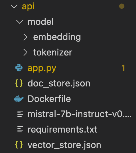
You should have downloaded the embeddings model and tokenizer above. Place these at the same level as your application code, requirements, and Dockerfile. You can download the LLM here.

You should have the following directory structure:

app.py

from flask import Flask, request, jsonify
import numpy as np
import json
from typing import Dict, List, Any
from llama_cpp import Llama
import torch
import logging
from transformers import AutoModel, AutoTokenizer

app = Flask(__name__)

# Set the logger level for Flask's logger
app.logger.setLevel(logging.INFO)

def compute_embeddings(text):
    tokenizer = AutoTokenizer.from_pretrained("/app/model/tokenizer") 
    model = AutoModel.from_pretrained("/app/model/embedding")

    inputs = tokenizer(text, return_tensors="pt", padding=True, truncation=True) 
    
    # Generate the embeddings 
    with torch.no_grad():    
        embeddings = model(**inputs).last_hidden_state.mean(dim=1).squeeze()

    return embeddings.tolist()

def compute_matches(vector_store, query_str, top_k):
    """
    This function takes in a vector store dictionary, a query string, and an int 'top_k'.
    It computes embeddings for the query string and then calculates the cosine similarity against every chunk embedding in the dictionary.
    The top_k matches are returned based on the highest similarity scores.
    """
    # Get the embedding for the query string
    query_str_embedding = np.array(compute_embeddings(query_str))
    scores = {}

    # Calculate the cosine similarity between the query embedding and each chunk's embedding
    for doc_id, chunks in vector_store.items():
        for chunk_id, chunk_embedding in chunks.items():
            chunk_embedding_array = np.array(chunk_embedding)
            # Normalize embeddings to unit vectors for cosine similarity calculation
            norm_query = np.linalg.norm(query_str_embedding)
            norm_chunk = np.linalg.norm(chunk_embedding_array)
            if norm_query == 0 or norm_chunk == 0:
                # Avoid division by zero
                score = 0
            else:
                score = np.dot(chunk_embedding_array, query_str_embedding) / (norm_query * norm_chunk)

            # Store the score along with a reference to both the document and the chunk
            scores[(doc_id, chunk_id)] = score

    # Sort scores and return the top_k results
    sorted_scores = sorted(scores.items(), key=lambda item: item[1], reverse=True)[:top_k]
    top_results = [(doc_id, chunk_id, score) for ((doc_id, chunk_id), score) in sorted_scores]

    return top_results

def open_json(path):
    with open(path, 'r') as f:
        data = json.load(f)
    return data

def retrieve_docs(doc_store, matches):
    top_match = matches[0]
    doc_id = top_match[0]
    chunk_id = top_match[1]
    docs = doc_store[doc_id][chunk_id]
    return docs

def construct_prompt(system_prompt, retrieved_docs, user_query):
    prompt = f"""{system_prompt}

    Here is the retrieved context:
    {retrieved_docs}

    Here is the users query:
    {user_query}
    """
    return prompt

@app.route('/rag_endpoint', methods=['GET', 'POST'])
def main():
    app.logger.info('Processing HTTP request')

    # Process the request
    query_str = request.args.get('query') or (request.get_json() or {}).get('query')
    if not query_str:
        return jsonify({"error":"missing required parameter 'query'"})

    vec_store = open_json('/app/vector_store.json')
    doc_store = open_json('/app/doc_store.json')

    matches = compute_matches(vector_store=vec_store, query_str=query_str, top_k=3)
    retrieved_docs = retrieve_docs(doc_store, matches)

    system_prompt = """
    You are an intelligent search engine. You will be provided with some retrieved context, as well as the users query.

    Your job is to understand the request, and answer based on the retrieved context.
    """

    base_prompt = construct_prompt(system_prompt=system_prompt, retrieved_docs=retrieved_docs, user_query=query_str)

    app.logger.info(f'constructed prompt: {base_prompt}')

    # Formatting the base prompt
    formatted_prompt = f"Q: {base_prompt} A: "
    
    llm = Llama(model_path="/app/mistral-7b-instruct-v0.2.Q3_K_L.gguf")
    response = llm(formatted_prompt, max_tokens=800, stop=["Q:", "n"], echo=False, stream=False)

    return jsonify({"response": response})

if __name__ == '__main__':
    app.run(host='0.0.0.0', port=5001)

Dockerfile

# Use an official Python runtime as a parent image
FROM --platform=linux/arm64 python:3.11

# Set the working directory in the container to /app
WORKDIR /app

# Copy the requirements file
COPY requirements.txt .

# Update system packages, install gcc and Python dependencies
RUN apt-get update && 
    apt-get install -y gcc g++ make libtool && 
    apt-get upgrade -y && 
    apt-get clean && 
    rm -rf /var/lib/apt/lists/* && 
    pip install --no-cache-dir -r requirements.txt

# Copy the current directory contents into the container at /app
COPY . /app

# Expose port 5001 to the outside world
EXPOSE 5001

# Run script when the container launches
CMD ["python", "app.py"]

Something important to note — we are setting the working directory to ‘/app’ in the second line of the Dockerfile. So any local paths (models, vector or document store), should be prefixed with ‘/app’ in your application code.

Also, when you run the app in the container (on a Mac), it will not be able to access the GPU, see this thread. I’ve noticed it usually takes about 20 minutes to get a response using the CPU.

Build & run:

docker build -t <image-name>:<tag> .

docker run -p 5001:5001 <image-name>:<tag>

Running the container automatically launches the app (see last line of the Dockerfile). You can now access your endpoint at the following URL:

http://127.0.0.1:5001/rag_endpoint

Call the API:

import requests, json

def call_api(query):
    URL = "http://127.0.0.1:5001/rag_endpoint"
    
    # Headers for the request
    headers = {
        "Content-Type": "application/json"
    }

    # Body for the request.
    body = {"query": query}

    # Making the POST request
    response = requests.post(URL, headers=headers, data=json.dumps(body))
    
    # Check if the request was successful
    if response.status_code == 200:
        return response.json()
    else:
        return f"Error: {response.status_code}, Message: {response.text}"

# Test
query = "Wall-mounted electric fireplace with realistic LED flames"

result = call_api(query)
print(result)

# result
{'response': {'choices': [{'finish_reason': 'stop', 'index': 0, 'logprobs': None, 'text': ' Based on the retrieved context, the wall-mounted electric fireplace mentioned includes features such as realistic LED flames. Therefore, the answer to the user's query "Wall-mounted electric fireplace with realistic LED flames" is a match to the retrieved context. The specific model mentioned in the context is manufactured by Hearth & Home and comes with additional heat settings.'}], 'created': 1715307125, 'id': 'cmpl-dd6c41ee-7c89-440f-9b04-0c9da9662f26', 'model': '/app/mistral-7b-instruct-v0.2.Q3_K_L.gguf', 'object': 'text_completion', 'usage': {'completion_tokens': 78, 'prompt_tokens': 177, 'total_tokens': 255}}}

Conclusion

I want to recap on the all the steps required to get to this point, and the workflow to retrofit this for any data / embeddings / LLM.

1. Pass your directory of text files to the document_chunker function to create the document store.
2. Choose your embeddings model. Save it locally.
3. Convert document store to vector store. Save both locally.
4. Download LLM from HF hub.
5. Move the files to the app directory (embeddings model, LLM, doc store and vec store JSON files).
6. Build and run Docker container.

Essentially it can be boiled down to this — use the build notebook to generate the doc_store and vector_store, and place these in your app.

GitHub here. Thank you for reading!

Local RAG From Scratch was originally published in Towards Data Science on Medium, where people are continuing the conversation by highlighting and responding to this story.

Machine Learning on GCP: from Notebooks to Pipelines

Notebooks are not enough for ML at scale

All images, unless otherwise noted, are by the author

Advocating for AI

There is a misunderstanding (not to say fantasy) which keeps coming back in companies whenever it comes to AI and Machine Learning. People often misjudge the complexity and the skills needed to bring Machine Learning projects to production, either because they do not understand the job, or (even worse) because they think they understand it, whereas they don’t.

Their first reaction when discovering AI might be something like “AI is actually pretty simple, I just need a Jupyter Notebook, copy paste code from here and there — or ask Copilot — and boom. No need to hire Data Scientists after all…” And the story always end badly, with bitterness, disappointment and a feeling that AI is a scam: difficulty to move to production, data drift, bugs, unwanted behavior.

So let’s write it down once and for all: AI/Machine Learning/any data-related job, is a real job, not a hobby. It requires skills, craftsmanship, and tools. If you think you can do ML in production with notebooks, you are wrong.

This article aims at showing, with a simple example, all the effort, skills and tools, it takes to move from a notebook to a real pipeline in production. Because ML in production is, mostly, about being able to automate the run of your code on a regular basis, with automation and monitoring.

And for those who are looking for an end-to-end “notebook to vertex pipelines” tutorial, you might find this helpful.

A simple use case

Let’s imagine you are a Data Scientist working at an e-commerce company. Your company is selling clothes online, and the marketing team asks for your help: they are preparing a special offer for specific products, and they would like to efficiently target customers by tailoring email content that will be pushed to them to maximize conversion. Your job is therefore simple: each customer should be assigned a score which represents the probability he/she purchases a product from the special offer.

The special offer will specifically target those brands, meaning that the marketing team wants to know which customers will buy their next product from the below brands:

Allegra K, Calvin Klein, Carhartt, Hanes, Volcom, Nautica, Quiksilver, Diesel, Dockers, Hurley

We will, for this article, use a publicly available dataset from Google, the `thelook_ecommerce` dataset. It contains fake data with transactions, customer data, product data, everything we would have at our disposal when working at an online fashion retailer.

To follow this notebook, you will need access to Google Cloud Platform, but the logic can be replicated to other Cloud providers or third-parties like Neptune, MLFlow, etc.

As a respectable Data Scientist, you start by creating a notebook which will help us in exploring the data.

We first import libraries which we will use during this article:

import catboost as cb
import pandas as pd
import sklearn as sk
import numpy as np
import datetime as dt

from dataclasses import dataclass
from sklearn.model_selection import train_test_split
from google.cloud import bigquery

%load_ext watermark
%watermark --packages catboost,pandas,sklearn,numpy,google.cloud.bigquery

catboost             : 1.0.4
pandas               : 1.4.2
numpy                : 1.22.4
google.cloud.bigquery: 3.2.0

Before Production

Getting and preparing the data

We will then load the data from BigQuery using the Python Client. Be sure to use your own project id:

query = """
    SELECT 
      transactions.user_id,
      products.brand,
      products.category,
      products.department,
      products.retail_price,
      users.gender,
      users.age,
      users.created_at,
      users.country,
      users.city,
      transactions.created_at
    FROM `bigquery-public-data.thelook_ecommerce.order_items` as transactions
    LEFT JOIN `bigquery-public-data.thelook_ecommerce.users` as users
      ON transactions.user_id = users.id
    LEFT JOIN `bigquery-public-data.thelook_ecommerce.products` as products
      ON transactions.product_id = products.id
    WHERE status <> 'Cancelled'
"""

client = bigquery.Client()
df = client.query(query).to_dataframe()

You should see something like that when looking at the dataframe:

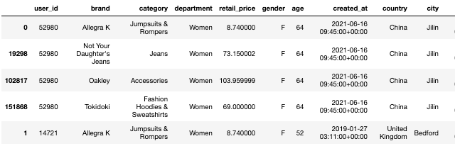
These represent the transactions / purchases made by the customers, enriched with customer and product information.

Given our objective is to predict which brand customers will buy in their next purchase, we will proceed as follows:

1. Group purchases chronologically for each customer
2. If a customer has N purchases, we consider the Nth purchase as the target, and the N-1 as our features.
3. We therefore exclude customers with only 1 purchase

Let’s put that into code:

# Compute recurrent customers
recurrent_customers = df.groupby('user_id')['created_at'].count().to_frame("n_purchases")

# Merge with dataset and filter those with more than 1 purchase
df = df.merge(recurrent_customers, left_on='user_id', right_index=True, how='inner')
df = df.query('n_purchases > 1')

# Fill missing values
df.fillna('NA', inplace=True)

target_brands = [
    'Allegra K', 
    'Calvin Klein', 
    'Carhartt', 
    'Hanes', 
    'Volcom', 
    'Nautica', 
    'Quiksilver', 
    'Diesel',
    'Dockers', 
    'Hurley'
]

aggregation_columns = ['brand', 'department', 'category']

# Group purchases by user chronologically
df_agg = (df.sort_values('created_at')
          .groupby(['user_id', 'gender', 'country', 'city', 'age'], as_index=False)[['brand', 'department', 'category']]
          .agg({k: ";".join for k in ['brand', 'department', 'category']})
         )

# Create the target
df_agg['last_purchase_brand'] = df_agg['brand'].apply(lambda x: x.split(";")[-1])
df_agg['target'] = df_agg['last_purchase_brand'].isin(target_brands)*1

df_agg['age'] = df_agg['age'].astype(float)

# Remove last item of sequence features to avoid target leakage :
for col in aggregation_columns:
    df_agg[col] = df_agg[col].apply(lambda x: ";".join(x.split(";")[:-1]))

Notice how we removed the last item in the sequence features: this is very important as otherwise we get what we call a “data leakeage”: the target is part of the features, the model is given the answer when learning.

We now get this new df_agg dataframe:

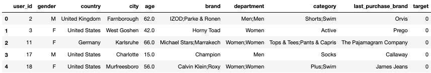
Comparing with the original dataframe, we see that user_id 2 has indeed purchased IZOD, Parke & Ronen, and finally Orvis which is not in the target brands.

Splitting into train, validation and test

As a seasoned Data Scientist, you will now split your data into different sets, as you obviously know that all three are required to perform some rigorous Machine Learning. (Cross-validation is out of the scope for today folks, let’s keep it simple.)

One key thing when splitting the data is to use the not-so-well-known stratify parameter from the scikit-learn train_test_split() method. The reason for that is because of class-imbalance: if the target distribution (% of 0 and 1 in our case) differs between training and testing, we might get frustrated with poor results when deploying the model. ML 101 kids: keep you data distributions as similar as possible between training data and test data.

# Remove unecessary features

df_agg.drop('last_purchase_category', axis=1, inplace=True)
df_agg.drop('last_purchase_brand', axis=1, inplace=True)
df_agg.drop('user_id', axis=1, inplace=True)

# Split the data into train and eval
df_train, df_val = train_test_split(df_agg, stratify=df_agg['target'], test_size=0.2)
print(f"{len(df_train)} samples in train")

df_train, df_val = train_test_split(df_agg, stratify=df_agg['target'], test_size=0.2)
print(f"{len(df_train)} samples in train") 
# 30950 samples in train

df_val, df_test = train_test_split(df_val, stratify=df_val['target'], test_size=0.5)
print(f"{len(df_val)} samples in val")
print(f"{len(df_test)} samples in test")
# 3869 samples in train
# 3869 samples in test

Now this is done, we will gracefully split our dataset between features and targets:

X_train, y_train = df_train.iloc[:, :-1], df_train['target']
X_val, y_val = df_val.iloc[:, :-1], df_val['target']
X_test, y_test = df_test.iloc[:, :-1], df_test['target']

Among the feature are different types. We usually separate those between:

• numerical features: they are continuous, and reflect a measurable, or ordered, quantity.
• categorical features: they are usually discrete, and are often represented as strings (ex: a country, a color, etc…)
• text features: they are usually sequences of words.

Of course there can be more like image, video, audio, etc.

The model: introducing CatBoost

For our classification problem (you already knew we were in a classification framework, didn’t you?), we will use a simple yet very powerful library: CatBoost. It is built and maintained by Yandex, and provides a high-level API to easily play with boosted trees. It is close to XGBoost, though it does not work exactly the same under the hood.

CatBoost offers a nice wrapper to deal with features from different kinds. In our case, some features can be considered as “text” as they are the concatenation of words, such as “Calvin Klein;BCBGeneration;Hanes”. Dealing with this type of features can sometimes be painful as you need to handle them with text splitters, tokenizers, lemmatizers, etc. Hopefully, CatBoost can manage everything for us!

# Define features
features = {
    'numerical': ['retail_price', 'age'],
    'static': ['gender', 'country', 'city'],
    'dynamic': ['brand', 'department', 'category']
}

# Build CatBoost "pools", which are datasets
train_pool = cb.Pool(
    X_train,
    y_train,
    cat_features=features.get("static"),
    text_features=features.get("dynamic"),
)

validation_pool = cb.Pool(
    X_val,
    y_val,
    cat_features=features.get("static"),
    text_features=features.get("dynamic"),
)

# Specify text processing options to handle our text features
text_processing_options = {
    "tokenizers": [
        {"tokenizer_id": "SemiColon", "delimiter": ";", "lowercasing": "false"}
    ],
    "dictionaries": [{"dictionary_id": "Word", "gram_order": "1"}],
    "feature_processing": {
        "default": [
            {
                "dictionaries_names": ["Word"],
                "feature_calcers": ["BoW"],
                "tokenizers_names": ["SemiColon"],
            }
        ],
    },
}

We are now ready to define and train our model. Going through each and every parameter is out of today’s scope as the number of parameters is quite impressive, but feel free to check the API yourself.

And for brevity, we will not perform hyperparameter tuning today, but this is obviously a large part of the Data Scientist’s job!

# Train the model
model = cb.CatBoostClassifier(
    iterations=200,
    loss_function="Logloss",
    random_state=42,
    verbose=1,
    auto_class_weights="SqrtBalanced",
    use_best_model=True,
    text_processing=text_processing_options,
    eval_metric='AUC'
)

model.fit(
    train_pool, 
    eval_set=validation_pool, 
    verbose=10
)

And voila, our model is trained. Are we done?

No. We need to check that our model’s performance between training and testing is consistent. A huge gap between training and testing means our model is overfitting (i.e. “learning the training data by heart and not good at predicting unseen data”).

For our model evaluation, we will use the ROC-AUC score. Not deep-diving on this one either, but from my own experience this is a generally quite robust metric and way better than accuracy.

A quick side note on accuracy: I usually do not recommend using this as your evaluation metric. Think of an imbalanced dataset where you have 1% of positives and 99% of negatives. What would be the accuracy of a very dumb model predicting 0 all the time? 99%. So accuracy not helpful here.

from sklearn.metrics import roc_auc_score

print(f"ROC-AUC for train set      : {roc_auc_score(y_true=y_train, y_score=model.predict(X_train)):.2f}")
print(f"ROC-AUC for validation set : {roc_auc_score(y_true=y_val, y_score=model.predict(X_val)):.2f}")
print(f"ROC-AUC for test set       : {roc_auc_score(y_true=y_test, y_score=model.predict(X_test)):.2f}")

ROC-AUC for train set      : 0.612
ROC-AUC for validation set : 0.586
ROC-AUC for test set       : 0.622

To be honest, 0.62 AUC is not great at all and a little bit disappointing for the expert Data Scientist you are. Our model definitely needs a little bit of parameter tuning here, and maybe we should also perform feature engineering more seriously.

But it is already better than random predictions (phew):

# random predictions

print(f"ROC-AUC for train set      : {roc_auc_score(y_true=y_train, y_score=np.random.rand(len(y_train))):.3f}")
print(f"ROC-AUC for validation set : {roc_auc_score(y_true=y_val, y_score=np.random.rand(len(y_val))):.3f}")
print(f"ROC-AUC for test set       : {roc_auc_score(y_true=y_test, y_score=np.random.rand(len(y_test))):.3f}")

ROC-AUC for train set      : 0.501
ROC-AUC for validation set : 0.499
ROC-AUC for test set       : 0.501

Let’s assume we are satisfied for now with our model and our notebook. This is where amateur Data Scientists would stop. So how do we make the next step and become production ready?

Moving to Production

Meet Docker

Docker is a set of platform as a service products that use OS-level virtualization to deliver software in packages called containers. This being said, think of Docker as code which can run everywhere, and allowing you to avoid the “works on your machine but not on mine” situation.

Why use Docker? Because among cool things such as being able to share your code, keep versions of it and ensure its easy deployment everywhere, it can also be used to build pipelines. Bear with me and you will understand as we go.

The first step to building a containerized application is to refactor and clean up our messy notebook. We are going to define 2 files, preprocess.py and train.py for our very simple example, and put them in a src directory. We will also include our requirements.txt file with everything in it.

# src/preprocess.py

from sklearn.model_selection import train_test_split
from google.cloud import bigquery

def create_dataset_from_bq():
    query = """
        SELECT 
          transactions.user_id,
          products.brand,
          products.category,
          products.department,
          products.retail_price,
          users.gender,
          users.age,
          users.created_at,
          users.country,
          users.city,
          transactions.created_at
        FROM `bigquery-public-data.thelook_ecommerce.order_items` as transactions
        LEFT JOIN `bigquery-public-data.thelook_ecommerce.users` as users
          ON transactions.user_id = users.id
        LEFT JOIN `bigquery-public-data.thelook_ecommerce.products` as products
          ON transactions.product_id = products.id
        WHERE status <> 'Cancelled'
    """
    client = bigquery.Client(project='<replace_with_your_project_id>')
    df = client.query(query).to_dataframe()
    print(f"{len(df)} rows loaded.")
    
    # Compute recurrent customers
    recurrent_customers = df.groupby('user_id')['created_at'].count().to_frame("n_purchases")

    # Merge with dataset and filter those with more than 1 purchase
    df = df.merge(recurrent_customers, left_on='user_id', right_index=True, how='inner')
    df = df.query('n_purchases > 1')

    # Fill missing value
    df.fillna('NA', inplace=True)

    target_brands = [
        'Allegra K', 
        'Calvin Klein', 
        'Carhartt', 
        'Hanes', 
        'Volcom', 
        'Nautica', 
        'Quiksilver', 
        'Diesel',
        'Dockers', 
        'Hurley'
    ]

    aggregation_columns = ['brand', 'department', 'category']

    # Group purchases by user chronologically
    df_agg = (df.sort_values('created_at')
              .groupby(['user_id', 'gender', 'country', 'city', 'age'], as_index=False)[['brand', 'department', 'category']]
              .agg({k: ";".join for k in ['brand', 'department', 'category']})
             )
    
    # Create the target
    df_agg['last_purchase_brand'] = df_agg['brand'].apply(lambda x: x.split(";")[-1])
    df_agg['target'] = df_agg['last_purchase_brand'].isin(target_brands)*1
    
    df_agg['age'] = df_agg['age'].astype(float)
    
    # Remove last item of sequence features to avoid target leakage :
    for col in aggregation_columns:
        df_agg[col] = df_agg[col].apply(lambda x: ";".join(x.split(";")[:-1]))
    
    df_agg.drop('last_purchase_category', axis=1, inplace=True)
    df_agg.drop('last_purchase_brand', axis=1, inplace=True)
    df_agg.drop('user_id', axis=1, inplace=True)
    return df_agg
    
    
def make_data_splits(df_agg):

    df_train, df_val = train_test_split(df_agg, stratify=df_agg['target'], test_size=0.2)
    print(f"{len(df_train)} samples in train")

    df_val, df_test = train_test_split(df_val, stratify=df_val['target'], test_size=0.5)
    print(f"{len(df_val)} samples in val")
    print(f"{len(df_test)} samples in test")
    
    return df_train, df_val, df_test

# src/train.py

import catboost as cb
import pandas as pd
import sklearn as sk
import numpy as np
import argparse

from sklearn.metrics import roc_auc_score
        
        
def train_and_evaluate(
        train_path: str,
        validation_path: str,
        test_path: str
    ):
    df_train = pd.read_csv(train_path)
    df_val = pd.read_csv(validation_path)
    df_test = pd.read_csv(test_path)
    
    df_train.fillna('NA', inplace=True)
    df_val.fillna('NA', inplace=True)
    df_test.fillna('NA', inplace=True)

    X_train, y_train = df_train.iloc[:, :-1], df_train['target']
    X_val, y_val = df_val.iloc[:, :-1], df_val['target']
    X_test, y_test = df_test.iloc[:, :-1], df_test['target']

    features = {
        'numerical': ['retail_price', 'age'],
        'static': ['gender', 'country', 'city'],
        'dynamic': ['brand', 'department', 'category']
    }

    train_pool = cb.Pool(
        X_train,
        y_train,
        cat_features=features.get("static"),
        text_features=features.get("dynamic"),
    )

    validation_pool = cb.Pool(
        X_val,
        y_val,
        cat_features=features.get("static"),
        text_features=features.get("dynamic"),
    )
    
    test_pool = cb.Pool(
        X_test,
        y_test,
        cat_features=features.get("static"),
        text_features=features.get("dynamic"),
    )


    params = CatBoostParams()

    text_processing_options = {
        "tokenizers": [
            {"tokenizer_id": "SemiColon", "delimiter": ";", "lowercasing": "false"}
        ],
        "dictionaries": [{"dictionary_id": "Word", "gram_order": "1"}],
        "feature_processing": {
            "default": [
                {
                    "dictionaries_names": ["Word"],
                    "feature_calcers": ["BoW"],
                    "tokenizers_names": ["SemiColon"],
                }
            ],
        },
    }

    # Train the model
    model = cb.CatBoostClassifier(
        iterations=200,
        loss_function="Logloss",
        random_state=42,
        verbose=1,
        auto_class_weights="SqrtBalanced",
        use_best_model=True,
        text_processing=text_processing_options,
        eval_metric='AUC'
    )


    model.fit(
        train_pool, 
        eval_set=validation_pool, 
        verbose=10
    )
    
    roc_train = roc_auc_score(y_true=y_train, y_score=model.predict(X_train))
    roc_eval  = roc_auc_score(y_true=y_val, y_score=model.predict(X_val))
    roc_test  = roc_auc_score(y_true=y_test, y_score=model.predict(X_test))
    print(f"ROC-AUC for train set      : {roc_train:.2f}")
    print(f"ROC-AUC for validation set : {roc_eval:.2f}")
    print(f"ROC-AUC for test.      set : {roc_test:.2f}")
    
    return {"model": model, "scores": {"train": roc_train, "eval": roc_eval, "test": roc_test}}

if __name__ == '__main__':
    parser = argparse.ArgumentParser()
    parser.add_argument("--train-path", type=str)
    parser.add_argument("--validation-path", type=str)
    parser.add_argument("--test-path", type=str)
    parser.add_argument("--output-dir", type=str)
    args, _ = parser.parse_known_args()
    _ = train_and_evaluate(
        args.train_path,
        args.validation_path,
        args.test_path)

Much cleaner now. You can actually launch your script from the command line now!

$ python train.py --train-path xxx --validation-path yyy etc.

We are now ready to build our Docker image. For that we need to write a Dockerfile at the root of the project:

# Dockerfile

FROM python:3.8-slim
WORKDIR /
COPY requirements.txt /requirements.txt
COPY src /src
RUN pip install --upgrade pip && pip install -r requirements.txt
ENTRYPOINT [ "bash" ]

This will take our requirements, copy the src folder and its contents, and install the requirements with pip when the image will build.

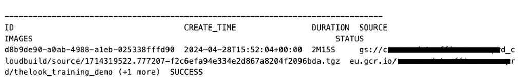
To build and deploy this image to a container registry, we can use the Google Cloud SDK and the gcloud commands:

PROJECT_ID = ...
IMAGE_NAME=f'thelook_training_demo'
IMAGE_TAG='latest'
IMAGE_URI='eu.gcr.io/{}/{}:{}'.format(PROJECT_ID, IMAGE_NAME, IMAGE_TAG)

!gcloud builds submit --tag $IMAGE_URI .

If everything goes well, you should see something like that:

Vertex Pipelines, the move to production

Docker images are the first step to doing some serious Machine Learning in production. The next step is building what we call “pipelines”. Pipelines are a series of operations orchestrated by a framework called Kubeflow. Kubeflow can run on Vertex AI on Google Cloud.

The reasons for preferring pipelines over notebooks in production can be debatable, but I will give you three based on my experience:

1. Monitoring and reproducibility: each pipeline is stored with its artefacts (datasets, models, metrics), meaning you can compare runs, re-run them, and audit them. Each time you re-run a notebook, you lose the history (or you have to manage artefacts yourself as weel as the logs. Good luck.)
2. Costs: Running a notebook implies having a machine on which it runs. — This machine has a cost, and for large models or huge datasets you will need virtual machines with heavy specs.
   — You have to remember to switch it off when you don’t use it.
   — Or you may simply crash your local machine if you choose not to use a virtual machine and have other applications running.
    — Vertex AI pipelines is a serverless service, meaning you do not have to manage the underlying infrastructure, and only pay for what you use, meaning the execution time.
3. Scalability: Good luck when running dozens of experiments on your local laptop simultaneously. You will roll back to using a VM, and scale that VM, and re-read the bullet point above.

The last reason to prefer pipelines over notebooks is subjective and highly debatable as well, but in my opinion notebooks are simply not designed for running workloads on a schedule. They are great though for exploration.

Use a cron job with a Docker image at least, or pipelines if you want to do things the right way, but never, ever, run a notebook in production.

Without further ado, let’s write the components of our pipeline:

# IMPORT REQUIRED LIBRARIES
from kfp.v2 import dsl
from kfp.v2.dsl import (Artifact,
                        Dataset,
                        Input,
                        Model,
                        Output,
                        Metrics,
                        Markdown,
                        HTML,
                        component, 
                        OutputPath, 
                        InputPath)
from kfp.v2 import compiler
from google.cloud.aiplatform import pipeline_jobs

%watermark --packages kfp,google.cloud.aiplatform

kfp                    : 2.7.0
google.cloud.aiplatform: 1.50.0

The first component will download the data from Bigquery and store it as a CSV file.

The BASE_IMAGE we use is the image we build previously! We can use it to import modules and functions we defined in our Docker image src folder:

@component(
    base_image=BASE_IMAGE,
    output_component_file="get_data.yaml"
)
def create_dataset_from_bq(
    output_dir: Output[Dataset],
):
    
    from src.preprocess import create_dataset_from_bq
    
    df = create_dataset_from_bq()
    
    df.to_csv(output_dir.path, index=False)

Next step: split data

@component(
    base_image=BASE_IMAGE,
    output_component_file="train_test_split.yaml",
)
def make_data_splits(
    dataset_full: Input[Dataset],
    dataset_train: Output[Dataset],
    dataset_val: Output[Dataset],
    dataset_test: Output[Dataset]):

    import pandas as pd
    from src.preprocess import make_data_splits

    df_agg = pd.read_csv(dataset_full.path)

    df_agg.fillna('NA', inplace=True)

    df_train, df_val, df_test = make_data_splits(df_agg)
    print(f"{len(df_train)} samples in train")
    print(f"{len(df_val)} samples in train")
    print(f"{len(df_test)} samples in test")
    
    df_train.to_csv(dataset_train.path, index=False)
    df_val.to_csv(dataset_val.path, index=False)
    df_test.to_csv(dataset_test.path, index=False)

Next step: model training. We will save the model scores to display them in the next step:

@component(
    base_image=BASE_IMAGE,
    output_component_file="train_model.yaml",
)
def train_model(
    dataset_train: Input[Dataset],
    dataset_val: Input[Dataset],
    dataset_test: Input[Dataset],
    model: Output[Model]
):

    import json
    from src.train import train_and_evaluate

    outputs = train_and_evaluate(
        dataset_train.path,
        dataset_val.path,
        dataset_test.path
    )
    cb_model = outputs['model']
    scores = outputs['scores']

    
    model.metadata["framework"] = "catboost" 
    # Save the model as an artifact
    with open(model.path, 'w') as f: 
        json.dump(scores, f)

The last step is computing the metrics (which are actually computed in the training of the model). It is merely necessary but is nice to show you how easy it is to build lightweight components. Notice how in this case we don’t build the component from the BASE_IMAGE (which can be quite large sometimes), but only build a lightweight image with necessary components:

@component(
    base_image="python:3.9",
    output_component_file="compute_metrics.yaml",
)
def compute_metrics(
    model: Input[Model],
    train_metric: Output[Metrics],
    val_metric: Output[Metrics],
    test_metric: Output[Metrics]
):
    
    import json
    
    file_name = model.path
    with open(file_name, 'r') as file:  
        model_metrics = json.load(file)
        
    train_metric.log_metric('train_auc', model_metrics['train'])
    val_metric.log_metric('val_auc', model_metrics['eval'])
    test_metric.log_metric('test_auc', model_metrics['test'])

There are usually other steps which we can include, like if we want to deploy our model as an API endpoint, but this is more advanced-level and requires crafting another Docker image for the serving of the model. To be covered next time.

Let’s now glue the components together:

# USE TIMESTAMP TO DEFINE UNIQUE PIPELINE NAMES
TIMESTAMP = dt.datetime.now().strftime("%Y%m%d%H%M%S")
DISPLAY_NAME = 'pipeline-thelook-demo-{}'.format(TIMESTAMP)
PIPELINE_ROOT = f"{BUCKET_NAME}/pipeline_root/"

# Define the pipeline. Notice how steps reuse outputs from previous steps
@dsl.pipeline(
    pipeline_root=PIPELINE_ROOT,
    # A name for the pipeline. Use to determine the pipeline Context.
    name="pipeline-demo"   
)

def pipeline(
    project: str = PROJECT_ID,
    region: str = REGION, 
    display_name: str = DISPLAY_NAME
):

    load_data_op = create_dataset_from_bq()
    train_test_split_op = make_data_splits(
        dataset_full=load_data_op.outputs["output_dir"]
    )
    train_model_op = train_model(
        dataset_train=train_test_split_op.outputs["dataset_train"], 
        dataset_val=train_test_split_op.outputs["dataset_val"],
        dataset_test=train_test_split_op.outputs["dataset_test"],
        )
    model_evaluation_op = compute_metrics(
        model=train_model_op.outputs["model"]
    )

# Compile the pipeline as JSON
compiler.Compiler().compile(
    pipeline_func=pipeline,
    package_path='thelook_pipeline.json'
)

# Start the pipeline
start_pipeline = pipeline_jobs.PipelineJob(
    display_name="thelook-demo-pipeline",
    template_path="thelook_pipeline.json",
    enable_caching=False,
    location=REGION,
    project=PROJECT_ID
)

# Run the pipeline
start_pipeline.run(service_account=<your_service_account_here>)

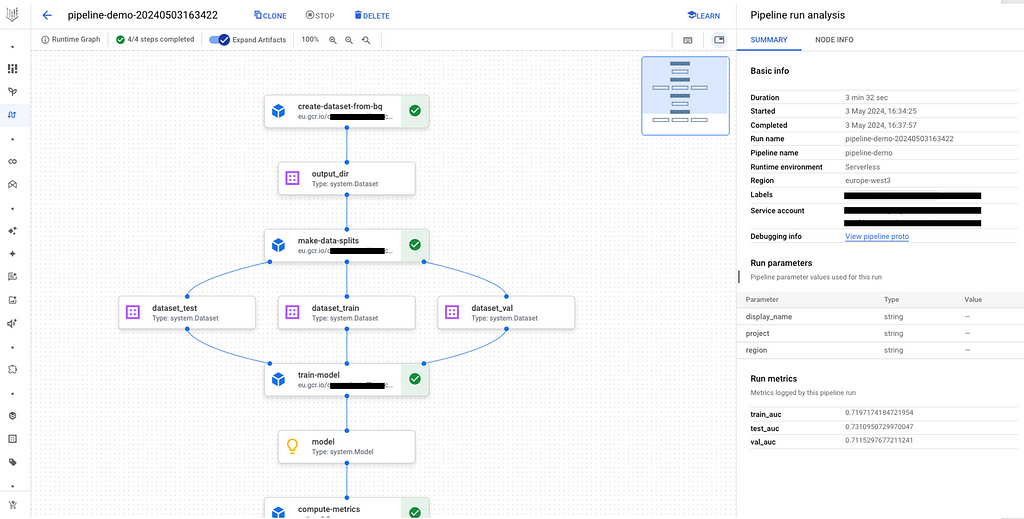
If everything works well, you will now see your pipeline in the Vertex UI:

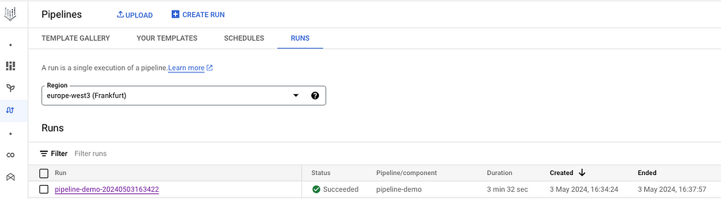
You can click on it and see the different steps:

Conclusion

Data Science, despite all the no-code/low-code enthusiasts telling you you don’t need to be a developer to do Machine Learning, is a real job. Like every job, it requires skills, concepts and tools which go beyond notebooks.

And for those who aspire to become Data Scientists, here is the reality of the job.

Happy coding.

Machine Learning on GCP : from dev to prod with Vertex AI was originally published in Towards Data Science on Medium, where people are continuing the conversation by highlighting and responding to this story.