Tag: AI

An interpretable classifier

Very often in when working on classification or regression problems in machine learning, we’re strictly interested in getting the most accurate model we can. In some cases, though, we’re interested also in the interpretability of the model. While models like XGBoost, CatBoost, and LGBM can be very strong models, it can be difficult to determine why they’ve made the predictions they have, or how they will behave with unseen data. These are what are called black-box models, models where we do not understand specifically why the make the predictions they do.

In many contexts this is fine; so long as we know they are reasonably accurate most of the time, they can be very useful, and it is understood they will be incorrect on occasion. For example, on a website, we may have a model that predicts which ads will be most likely to generate sales if shown to the current user. If the model behaves poorly on the rare occasion, this may affect revenues, but there are no major issues; we just have a model that’s sub-optimal, but generally useful.

But, in other contexts, it can be very important to know why the models make the predictions that they do. This includes high-stakes environments, such as in medicine and security. It also includes environments where we need to ensure there are no biases in the models related to race, gender or other protected classes. It’s important, as well, in environments that are audited: where it’s necessary to understand the models to determine they are performing as they should.

Even in these cases, it is sometimes possible to use black-box models (such as boosted models, neural networks, Random Forests and so on) and then perform what is called post-hoc analysis. This provides an explanation, after the fact, of why the model likely predicted as it did. This is the field of Explainable AI (XAI), which uses techniques such as proxy models, feature importances (e.g. SHAP), counterfactuals, or ALE plots. These are very useful tools, but, everything else equal, it is preferable to have a model that is interpretable in the first place, at least where possible. XAI methods are very useful, but they do have limitations.

With proxy models, we train a model that is interpretable (for example, a shallow decision tree) to learn the behavior of the black-box model. This can provide some level of explanation, but will not always be accurate and will provide only approximate explanations.

Feature importances are also quite useful, but indicate only what the relevant features are, not how they relate to the prediction, or how they interact with each other to form the prediction. They also have no ability to determine if the model will work reasonably with unseen data.

With interpretable models, we do not have these issues. The model is itself comprehensible and we can know exactly why it makes each prediction. The problem, though, is: interpretable models can have lower accuracy then black-box models. They will not always, but will often have lower accuracy. Most interpretable models, for most problems, will not be competitive with boosted models or neural networks. For any given problem, it may be necessary to try several interpretable models before an interpretable model of sufficient accuracy can be found, if any can be.

There are a number of interpretable models available today, but unfortunately, very few. Among these are decision trees, rules lists (and rule sets), GAMs (Generalized Additive Models, such as Explainable Boosted Machines), and linear/logistic regression. These can each be useful where they work well, but the options are limited. The implication is: it can be impossible for many projects to find an interpretable model that performs satisfactorily. There can be real benefits in having more options available.

We introduce here another interpretable model, called ikNN, or interpretable k Nearest Neighbors. This is based on an ensemble of 2d kNN models. While the idea is straightforward, it is also surprisingly effective. And quite interpretable. While it is not competitive in terms of accuracy with state of the art models for prediction on tabular data such as CatBoost, it can often provide accuracy that is close and that is sufficient for the problem. It is also quite competitive with decision trees and other existing interpretable models.

Interestingly, it also appears to have stronger accuracy than plain kNN models.

The main page for the project is: https://github.com/Brett-Kennedy/ikNN

The project defines a single class called iKNNClassifier. This can be included in any project copying the interpretable_knn.py file and importing it. It provides an interface consistent with scikit-learn classifiers. That is, we generally simply need to create an instance, call fit(), and call predict(), similar to using Random Forest or other scikit-learn models.

Using, under the hood, using an ensemble of 2d kNN’s provides a number of advantages. One is the normal advantage we always see with ensembling: we get more reliable predictions than when relying on a single model.

Another is that 2d spaces are straightforward to visualize. The model currently requires numeric input (as is the case with kNN), so all categorical features need to be encoded, but once this is done, every 2d space can be visualized as a scatter plot. This provides a high degree of interpretability.

And, it’s possible to determine the most relevant 2d spaces for each prediction, which allows us to present a small number of plots for each record. This allows fairly simple as well as complete visual explanations for each record.

ikNN is, then, an interesting model, as it is based on ensembling, but actually increases interpretability, while the opposite is more often the case.

Standard kNN Classifiers

kNN models are less-used than many others, as they are not usually as accurate as boosted models or neural networks, or as interpretable as decision trees. They are, though, still widely used. They work based on an intuitive idea: the class of an item can be predicted based on the class of most of the items that are most similar to it.

For example, if we look at the iris dataset (as is used in an example below), we have three classes, representing three types of iris. If we collect another sample of iris and wish to predict which of the three types of iris it is, we can look at the most similar, say, 10 records from the training data, determine what their classes are, and take the most common of these.

In this example, we chose 10 to be the number of nearest neighbors to use to estimate the class of each record, but other values may be used. This is specified as a hyperparameter (the k parameter) with kNN and ikNN models. We wish set k so as to use to a reasonable number of similar records. If we use too few, the results may be unstable (each prediction is based on very few other records). If we use too many, the results may be based on some other records that aren’t that similar.

We also need a way to determine which are the most similar items. For this, at least by default, we use the Euclidean distance. If the dataset has 20 features and we use k=10, then we find the closest 10 points in the 20-dimensional space, based on their Euclidean distances.

Predicting for one record, we would find the 10 closest records from the training data and see what their classes are. If 8 of the 10 are class Setosa (one of the 3 types of iris), then we can assume this row is most likely also Setosa, or at least this is the best guess we can make.

One issue with this is, it breaks down when there are many features, due to what’s called the curse of dimensionality. An interesting property of high-dimensional spaces is that with enough features, distances between the points start to become meaningless.

kNN also uses all features equally, though some may be much more predictive of the target than others. The distances between points, being based on Euclidean (or sometimes Manhattan or other distance metrics) are calculated considering all features equally. This is simple, but not always the most effective, given many features may be irrelevant to the target. Assuming some feature selection has been performed, this is less likely, but the relevance of the features will still not be equal.

And, the predictions made by kNN predictors are uninterpretable. The algorithm is quite intelligible, but the predictions can be difficult to understand. It’s possible to list the k nearest neighbors, which provides some insight into the predictions, but it’s difficult to see why a given set of records are the most similar, particularly where there are many features.

The ikNN Algorithm

The ikNN model first takes each pair of features and creates a standard 2d kNN classifier using these features. So, if a table has 10 features, this creates 10 choose 2, or 45 models, one for each unique pair of features.

It then assesses their accuracies with respect to predicting the target column using the training data. Given this, the ikNN model determines the predictive power of each 2d subspace. In the case of 45 2d models, some will be more predictive than others. To make a prediction, the 2d subspaces known to be most predictive are used, optionally weighted by their predictive power on the training data.

Further, at inference, the purity of the set of nearest neighbors around a given row within each 2d space may be considered, allowing the model to weight more heavily both the subspaces proven to be more predictive with training data and the subspaces that appear to be the most consistent in their prediction with respect to the current instance.

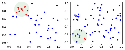
Consider two subspaces and a point shown here as a star. In both cases, we can find the set of k points closest to the point. Here we draw a green circle around the star, though the set of points do not actually form a circle (though there is a radius to the kth nearest neighbor that effectively defines a neighborhood).

These plots each represent a pair of features. In the case of the left plot, there is very high consistency among the neighbors of the star: they are entirely red. In the right plot, there is no little consistency among the neigbhors: some are red and some are blue. The first pair of features appears to be more predictive of the record than the second pair of features, which ikNN takes advantage of.

This approach allows the model to consider the influence all input features, but weigh them in a manner that magnifies the influence of more predictive features, and diminishes the influence of less-predictive features.

Example

We first demonstrate ikNN with a toy dataset, specifically the iris dataset. We load in the data, do a train-test split, and make predictions on the test set.

from sklearn.datasets import load_iris
from interpretable_knn import ikNNClassifier

iris = load_iris()
X, y = iris.data, iris.target

clf = ikNNClassifier()
X_train, X_test, y_train, y_test = train_test_split(
   X, y, test_size=0.33, random_state=42)
clf.fit(X_train, y_train)
y_pred = clf.predict(X_test)

For prediction, this is all that is required. But, ikNN also provides tools for understanding the model, specifically the graph_model() and graph_predictions() APIs.

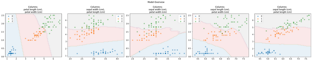
For an example of graph_model():

ikNN.graph_model(X.columns)

This provides a quick overview of the dataspace, plotting, by default, five 2d spaces. The dots show the classes of the training data. The background color shows the predictions made by the 2d kNN for each region of the 2d space.

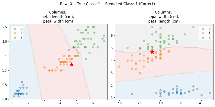
The graph_predictions() API will explain a specific row, for example:

Here, the row being explained is shown as a red star. Again, by default, five plots are used by default, but for simplicity, this uses just two. In both plots, we can see where Row 0 is located relative to the training data and the predictions made by the 2D kNN for this 2D space.

Visualizations

Although it is configurable, by default only five 2d spaces are used by each ikNN prediction. This ensures the prediction times are fast and the visualizations simple. It also means that the visualizations are showing the true predictions, not a simplification of the predictions, ensuring the predictions are completely interpretable

For most datasets, for most rows, all or almost all 2d spaces agree on the prediction. However, where the predictions are incorrect, it may be useful to examine more 2d plots in order to better tune the hyperparameters to suit the current dataset.

Accuracy Tests

A set of tests were performed using a random set of 100 classification datasets from OpenML. Comparing the F1 (macro) scores of standard kNN and ikNN models, ikNN had higher scores for 58 datasets and kNN for 42.

ikNN’s do even a bit better when performing grid search to search for the best hyperparameters. After doing this for both models on all 100 datasets, ikNN performed the best in 76 of the 100 cases. It also tends to have smaller gaps between the train and test scores, suggesting more stable models than standard kNN models.

ikNN models can be somewhat slower, but they tend to still be considerably faster than boosted models, and still very fast, typically taking well under a minute for training, usually only seconds.

The github page provides some more examples and analysis of the accuracy.

Conclusions

While ikNN is likely not the strongest model where accuracy is the primary goal (though, as with any model, it can be on occasion), it is likely a model that should be tried where an interpretable model is necessary.

This page provided the basic information necessary to use the tool. It simply necessary to download the .py file (https://github.com/Brett-Kennedy/ikNN/blob/main/ikNN/interpretable_knn.py), import it into your code, create an instance, train and predict, and (where desired), call graph_predictions() to view the explanations for any records you wish.

All images are by author.

---

Interpretable kNN (ikNN) was originally published in Towards Data Science on Medium, where people are continuing the conversation by highlighting and responding to this story.

Addressing compatibility issues during installation | ONNX for NVIDIA GPUs | Hugging Face’s Optimum library

This article discusses the ONNX runtime, one of the most effective ways of speeding up Stable Diffusion inference. On an A100 GPU, running SDXL for 30 denoising steps to generate a 1024 x 1024 image can be as fast as 2 seconds. However, the ONNX runtime depends on multiple moving pieces, and installing the right versions of all of its dependencies can be tricky in a constantly evolving ecosystem. Take this as a high-level debugging guide, where I share my struggles in hopes of saving you time. While the specific versions and commands might quickly become obsolete, the high-level concepts should remain relevant for a longer period of time.

What is ONNX?

ONNX can actually refer to two different (but related) parts of the ML stack:

1. ONNX is a format for storing machine learning models. It stands for Open Neural Network Exchange and, as its name suggests, its main goal is interoperability across platforms. ONNX is a self-contained format: it stores both the model weights and architecture. This means that a single .onnx file contains all the information needed to run inference. No need to write any additional code to define or load a model; instead, you simply pass it to a runtime (more on this below).
2. ONNX is also a runtime to run model that are in ONNX format. It literally runs the model. You can see it as a mediator between the architecture-agnostic ONNX format and the actual hardware that runs inference. There is a separate version of the runtime for each supported accelerator type (see full list here). Note, however, that the ONNX runtime is not the only way to run inference with a model that is in ONNX format — it’s just one way. Manufacturers can choose to build their own runtimes that are hyper-optimized for their hardware. For instance, NVIDIA’s TensorRT is an alternative to the ONNX runtime.

This article focuses on running Stable Diffusion models using the ONNX runtime. While the high-level concepts are probably timeless, note that the ML tooling ecosystem is in constant change, so the exact workflow or code snippets might become obsolete (this article was written in May 2024). I will focus on the Python implementation in particular, but note that the ONNX runtime can also operate in other languages like C++, C#, Java or JavaScript.

Pros of the ONNX Runtime

• Balance between inference speed and interoperability. While the ONNX runtime will not always be the fastest solution for all types of hardware, it is a fast enough solution for most types of hardware. This is particularly appealing if you’re serving your models on a heterogeneous fleet of machines and don’t have the resources to micro-optimize for each different accelerator.
• Wide adoption and reliable authorship. ONNX was open-sourced by Microsoft, who are still maintaining it. It is widely adopted and well integrated into the wider ML ecosystem. For instance, Hugging Face’s Optimum library allows you to define and run ONNX model pipelines with a syntax that is reminiscent of their popular transformers and diffusers libraries.

Cons of the ONNX Runtime

• Engineering overhead. Compared to the alternative of running inference directly in PyTorch, the ONNX runtime requires compiling your model to the ONNX format (which can take 20–30 minutes for a Stable Diffusion model) and installing the runtime itself.
• Restricted set of ops. The ONNX format doesn’t support all PyTorch operations (it is even more restrictive than TorchScript). If your model is using an unsupported operation, you will either have to reimplement the relevant portion, or drop ONNX altogether.
• Brittle installation and setup. Since the ONNX runtime makes the translation from the ONNX format to architecture-specific instructions, it can be tricky to get the right combination of software versions to make it work. For instance, if running on an NVIDIA GPU, you need to ensure compatibility of (1) operating system, (2) CUDA version, (3) cuDNN version, and (4) ONNX runtime version. There are useful resources like the CUDA compatibility matrix, but you might still end up wasting hours finding the magic combination that works at a given point in time.
• Hardware limitations. While the ONNX runtime can run on many architectures, it cannot run on all architectures like pure PyTorch models can. For instance, there is currently (May 2024) no support for Google Cloud TPUs or AWS Inferentia chips (see FAQ).

At first glance, the list of cons looks longer than the list of pros, but don’t be discouraged — as shown later on, the improvements in model latency can be significant and worth it.

How to install the ONNX runtime

Option #1: Install from source

As mentioned above, the ONNX runtime requires compatibility between many pieces of software. If you want to be on the cutting edge, the best way to get the latest version is to follow the instructions in the official Github repository. For Stable Diffusion in particular, this folder contains installation instructions and sample scripts for generating images. Expect building from source to take quite a while (around 30 minutes).

At the time of writing (May 2024), this solution worked seamlessly for me on an Amazon EC2 instance (g5.2xlarge, which comes with a A10G GPU). It avoids compatibility issues discussed below by using a Docker image that comes with the right dependencies.

Option #2: Install via PyPI

In production, you will most likely want a stable version of the ONNX runtime from PyPI, instead of installing the latest version from source. For Python in particular, there are two different libraries (one for CPU and one for GPU). Here is the command to install it for CPU:

pip install onnxruntime

And here is the command to install it for GPU:

pip install onnxruntime-gpu

You should never install both. Having them both might lead to error messages or behaviors that are not easy to track back to this root cause. The ONNX runtime might simply fail to acknowledge the presence of the GPU, which will look surprising given that onnxruntime-gpu is indeed installed.

Addressing compatibility issues

In an ideal world, pip install onnxruntime-gpu would be the end of the story. However, in practice, there are strong compatibility requirements between other pieces of software on your machine, including the operating system, the hardware-specific drivers, and the Python version.

Say that you want to use the latest version of the ONNX runtime (1.17.1) at the time of writing. So what stars do we need to align to make this happen?

Here are some of the most common sources of incompatibility that can help you set up your environment. The exact details will quickly become obsolete, but the high-level ideas should continue to apply for a while.

CUDA compatibility

If you are not planning on using an NVIDIA GPU, you can skip this section. CUDA is a platform for parallel computing that sits on top of NVIDIA GPUs, and is required for machine learning workflows. Each version of the ONNX runtime is compatible with only certain CUDA versions, as you can see in this compatibility matrix.

According to this matrix, the latest ONNX runtime version (1.17) is compatible with both CUDA 11.8 and CUDA 12. But you need to pay attention to the fine print: by default, ONNX runtime 1.17 expects CUDA 11.8. However, most VMs today (May 2024) come with CUDA 12.1 (you can check the version by running nvcc –version). For this particular setup, you’ll have to replace the usual pip install onnxruntime-gpu with:

pip install onnxruntime-gpu==1.17.1 --extra-index-url https://aiinfra.pkgs.visualstudio.com/PublicPackages/_packaging/onnxruntime-cuda-12/pypi/simple/

Note that, instead of being at the mercy of whatever CUDA version happens to be installed on your machine, a cleaner solution is to do your work from within a Docker container. You simply choose the image that has your desired version of Python and CUDA. For instance:

docker run --rm -it --gpus all nvcr.io/nvidia/pytorch:23.10-py3

OS + Python + pip compatibility

This section discusses compatibility issues that are architecture-agnostic (i.e. you’ll encounter them regardless of the target accelerator). It boils down to making sure that your software (operating system, Python installation and pip installation) are compatible with your desired version of the ONNX runtime library.

Pip version: Unless you are working with legacy code or systems, your safest bet is to upgrade pip to the latest version:

python -m pip install --upgrade pip

Python version: As of May 2024, the Python version that is least likely to give you headaches is 3.10 (this is what most VMs come with by default). Again, unless you are working with legacy code, you certainly want at least 3.8 (since 3.7 was deprecated in June 2023).

Operating system: The fact that the OS version can also hinder your ability to install the desired library came as a surprise to me, especially that I was using the most standard EC2 instances. And it wasn’t straightforward to figure out that the OS version was the culprit.

Here I will walk you through my debugging process, in the hopes that the workflow itself is longer-lived than the specifics of the versions today. First, I installed onnxruntime-gpu with the following command (since I had CUDA 12.1 installed on my machine):

pip install onnxruntime-gpu --extra-index-url https://aiinfra.pkgs.visualstudio.com/PublicPackages/_packaging/onnxruntime-cuda-12/pypi/simple/

On the surface, this should install the latest version of the library available on PyPI. In reality however, this will install the latest version compatible with your current setup (OS + Python version + pip version). For me at the time, that happened to be onnxruntime-gpu==1.16.0. (as opposed to 1.17.1, which is the latest). Unknowingly installing an older version simply manifested in the ONNX runtime being unable to detect the GPU, with no other clues. After somewhat accidentally discovering the version is older than expected, I explicitly asked for the newer one:

pip install onnxruntime-gpu==1.17.1 --extra-index-url https://aiinfra.pkgs.visualstudio.com/PublicPackages/_packaging/onnxruntime-cuda-12/pypi/simple/

This resulted in a message from pip complaining that the version I requested is not actually available (despite being listed on PyPI):

ERROR: Could not find a version that satisfies the requirement onnxruntime-gpu==1.17.1 (from versions: 1.12.0, 1.12.1, 1.13.1, 1.14.0, 1.14.1, 1.15.0, 1.15.1, 1.16.0, 1.16.1, 1.16.2, 1.16.3)
ERROR: No matching distribution found for onnxruntime-gpu==1.17.1

To understand why the latest version is not getting installed, you can pass a flag that makes pip verbose: pip install … -vvv. This reveals all the Python wheels that pip cycles through in order to find the newest one that is compatible to your system. Here is what the output looked like for me:

Skipping link: none of the wheel's tags (cp35-cp35m-manylinux1_x86_64) are compatible (run pip debug --verbose to show compatible tags): https://files.pythonhosted.org/packages/26/1a/163521e075d2e0c3effab02ba11caba362c06360913d7c989dcf9506edb9/onnxruntime_gpu-0.1.2-cp35-cp35m-manylinux1_x86_64.whl (from https://pypi.org/simple/onnxruntime-gpu/)
Skipping link: none of the wheel's tags (cp36-cp36m-manylinux1_x86_64) are compatible (run pip debug --verbose to show compatible tags): https://files.pythonhosted.org/packages/52/f2/30aaa83bc9e90e8a919c8e44e1010796eb30f3f6b42a7141ffc89aba9a8e/onnxruntime_gpu-0.1.2-cp36-cp36m-manylinux1_x86_64.whl (from https://pypi.org/simple/onnxruntime-gpu/)
Skipping link: none of the wheel's tags (cp37-cp37m-manylinux1_x86_64) are compatible (run pip debug --verbose to show compatible tags): https://files.pythonhosted.org/packages/a2/05/af0481897255798ee57a242d3989427015a11a84f2eae92934627be78cb5/onnxruntime_gpu-0.1.2-cp37-cp37m-manylinux1_x86_64.whl (from https://pypi.org/simple/onnxruntime-gpu/)
Skipping link: none of the wheel's tags (cp35-cp35m-manylinux1_x86_64) are compatible (run pip debug --verbose to show compatible tags): https://files.pythonhosted.org/packages/17/cb/0def5a44db45c6d38d95387f20057905ce2dd4fad35c0d43ee4b1cebbb19/onnxruntime_gpu-0.1.3-cp35-cp35m-manylinux1_x86_64.whl (from https://pypi.org/simple/onnxruntime-gpu/)
Skipping link: none of the wheel's tags (cp36-cp36m-manylinux1_x86_64) are compatible (run pip debug --verbose to show compatible tags): https://files.pythonhosted.org/packages/a6/53/0e733ebd72d7dbc84e49eeece15af13ab38feb41167fb6c3e90c92f09cbb/onnxruntime_gpu-0.1.3-cp36-cp36m-manylinux1_x86_64.whl (from https://pypi.org/simple/onnxruntime-gpu/)
...

The tags listed in brackets are Python platform compatibility tags, and you can read more about them here. In a nutshell, every Python wheel comes with a tag that indicates what system it can run on. For instance, cp35-cp35m-manylinux1_x86_64 requires CPython 3.5, a set of (older) Linux distributions that fall under the manylinux1 umbrella, and a 64-bit x86-compatible processor.

Since I wanted to run Python 3.10 on a Linux machine (hence filtering for cp310.*manylinux.*, I was left with a single possible wheel for the onnxruntime-gpu library, with the following tag:

cp310-cp310-manylinux_2_28_x86_64

You can get a list of tags that are compatible with your system by running pip debug –verbose. Here is what part of my output looked like:

cp310-cp310-manylinux_2_26_x86_64
cp310-cp310-manylinux_2_25_x86_64
cp310-cp310-manylinux_2_24_x86_64
cp310-cp310-manylinux_2_23_x86_64
cp310-cp310-manylinux_2_22_x86_64
cp310-cp310-manylinux_2_21_x86_64
cp310-cp310-manylinux_2_20_x86_64
cp310-cp310-manylinux_2_19_x86_64
cp310-cp310-manylinux_2_18_x86_64
cp310-cp310-manylinux_2_17_x86_64
...

In other words, my operating system is just a tad too old (the maximum linux tag that it supports is manylinux_2_26, while the onnxruntime-gpu library’s only Python 3.10 wheel requires manylinux_2_28. Upgrading from Ubuntu 20.04 to Ubuntu 24.04 solved the problem.

How to run Stable Diffusion with the ONNX runtime

Once the ONNX runtime is (finally) installed, generating images with Stable Diffusion requires two following steps:

1. Export the PyTorch model to ONNX (this can take > 30 minutes!)
2. Pass the ONNX model and the inputs (text prompt and other parameters) to the ONNX runtime.

Option #1: Using official scripts from Microsoft

As mentioned before, using the official sample scripts from the ONNX runtime repository worked out of the box for me. If you follow their installation instructions, you won’t even have to deal with the compatibility issues mentioned above. After installation, generating an image is a simple as:

python3 demo_txt2img_xl.py "starry night over Golden Gate Bridge by van gogh"

Under the hood, this script defines an SDXL model using Hugging Face’s diffusers library, exports it to ONNX format (which can take up to 30 minutes!), then invokes the ONNX runtime.

Option #2: Using Hugging Face’s Optimum library

The Optimum library promises a lot of convenience, allowing you to run models on various accelerators while using the familiar pipeline APIs from the well-known transformers and diffusers libraries. For ONNX in particular, this is what inference code for SDXL looks like (more in this tutorial):

from optimum.onnxruntime import ORTStableDiffusionXLPipeline

model_id = "stabilityai/stable-diffusion-xl-base-1.0"
base = ORTStableDiffusionXLPipeline.from_pretrained(model_id)
prompt = "sailing ship in storm by Leonardo da Vinci"
image = base(prompt).images[0]

# Don't forget to save the ONNX model
save_directory = "sd_xl_base"
base.save_pretrained(save_directory)

In practice, however, I struggled a lot with the Optimum library. First, installation is non-trivial; naively following the installation instruction in the README file will run into the incompatibility issues explained above. This is not Optimum’s fault per se, but it does add yet another layer of abstraction on top of an already brittle setup. The Optimum installation might pull a version of onnxruntime that is conflicting with your setup.

Even after I won the battle against compatibility issues, I wasn’t able to run SDXL inference on GPU using Optimum’s ONNX interface. The code snippet above (directly taken from a Hugging Face tutorial) fails with some shape mismatches, perhaps due to bugs in the PyTorch → ONNX conversion:

[ONNXRuntimeError] : 1 : FAIL : Non-zero status code returned while running Add node.
Name:'/down_blocks.1/attentions.0/Add'
Status Message: /down_blocks.1/attentions.0/Add: left operand cannot broadcast on dim 3 LeftShape: {2,64,4096,10}, RightShape: {2,640,64,64}

For a brief second I considered getting into the weeds and debugging the Hugging Face code (at least it’s open source!), but gave up when I realized that Optimum has a backlog of more than 250 issues, with issues going for weeks with no acknowledgement from the Hugging Face team. I decided to move on and simply use Microsoft’s official scripts instead.

Latency Reduction

As promised, the effort to get the ONNX runtime working is worth it. On an A100 GPU, the inference time is reduced from 7–8 seconds (when running vanilla PyTorch) to ~2 seconds. This is comparable to TensorRT (an NVIDIA-specific alternative to ONNX), and about 1 second faster than torch.compile (PyTorch’s native JIT compilation).

Reportedly, switching to even more performant GPUs (e.g. H100) can lead to even higher gains from running your model with a specialized runtime.

Conclusion and further reading

The ONNX runtime promises significant latency gains, but it comes with non-trivial engineering overhead. It also faces the classic trade-off for static compilation: inference is a lot faster, but the graph cannot be dynamically modified (which is at odds with dynamic adapters like peft). The ONNX runtime and similar compilation methods are worth adding to your pipeline once you’ve passed the experimentation phase, and are ready to invest in efficient production code.

If you’re interested in optimizing inference time, here are some articles that I found helpful:

• SDXL inference in under 2 seconds: the ultimate guide to Stable Diffusion optimization
• 40% faster Stable Diffusion XL inference with NVIDIA TensorRT
• Unlocking the full power of NVIDIA H100 GPUs for ML inference with TensorRT
• Making stable diffusion 25% faster using TensorRT
• Maximize Stable Diffusion performance and lower inference costs with AWS Inferentia2
• Generate images with Stable Diffusion models on AWS Inferentia
• Text-to-Image Generation with Stable Diffusion and OpenVINO
• Accelerating Stable Diffusion Inference on Intel CPUs

---

How to Run Stable Diffusion with ONNX was originally published in Towards Data Science on Medium, where people are continuing the conversation by highlighting and responding to this story.