Tag: AI

Welcome, developers! If you’ve spent time mastering data structures and algorithms, have you considered their encrypted data potential?

Introducing the world of Fully Homomorphic Encryption (FHE), a groundbreaking approach that allows for computations on encrypted data without ever needing to decrypt it. This means you can perform operations on data while maintaining complete privacy. This employs post-quantum cryptographic methods, allowing encrypted data to remain secure on public networks such as clouds or blockchains.

In this series of articles, we explore how traditional data structures and algorithms, like binary search trees, sorting algorithms, and even dynamic programming techniques, can be implemented in an encrypted domain using FHE. Imagine performing a binary search on a dataset that remains entirely encrypted, or sorting data that is not visible in its raw form, all while ensuring that the privacy and security of the data are never compromised.

We’ll dive into how FHE works at a fundamental level and the implications it has for both data security and algorithm design. Later in this series we’ll also explore real-world applications and the potential challenges developers face when implementing these encrypted algorithms, such as fraud detection, payments, and more. This isn’t just about enhancing security; it’s about rethinking how we interact with data and pushing the boundaries of what’s possible in software development.

Whether you’re a seasoned developer or new to the concept of encrypted computing, this article will provide you with insights into how you can integrate advanced cryptographic techniques into your programming projects. Let’s embark on this journey together and unlock the potential of coding in cipher, transforming everyday data operations into secure, privacy-preserving computations that pave the way for a new era of secure digital innovation.

Fully Homomorphic Encryption Basics

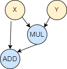
The two primary types of operations that can be performed on ciphertexts in FHE are addition and multiplication, though these serve as building blocks for more complex operations. For instance, you can add two encrypted values, and the result, when decrypted, will be the sum of the original plaintext values. Complex computations can be constructed using combinations of these basic operations, allowing for algorithms and functions to be executed on encrypted data. For example, we have a function F that takes two input values x and y and computes x + x * y. A mathematical representation of this function is written as F(x, y) = x + x * y, which can also be represented as a circuit, which is in other words, a direct acyclic graph:

Noise

While FHE allows computations on encrypted data, it comes with the added challenge of noise growth within ciphertexts, which can eventually lead to decryption errors if not properly managed. In FHE schemes, every ciphertext includes some amount of noise that ensures security. This noise is small initially but grows as more operations are performed on the ciphertext. When performing an addition operation, the noise is relatively small, however, when multiplying, the noise from each of the two ciphertexts multiplies together in the product. This in turn results in a much higher noise level. Specifically, if you multiply two ciphertexts with noise levels n1 and n2, the noise in the resulting ciphertext can be approximated as n1 * n2, or a function growing much faster than either n1 or n2 alone.

There are a few ways to mange the noise in FHE schemas, but for the sake of article length, the main focus is on the noise reduction technique called bootstrapping. Bootstrapping reduces the noise level of a ciphertext, thus restoring the noise budget and allowing more computations. Essentially, bootstrapping applies the decryption and re-encryption algorithms homomorphically. This requires evaluating the entire decryption circuit of the FHE scheme as an encrypted function. The output is a new ciphertext that represents the same plaintext as before but with reduced noise. Bootstrapping is a critical technique in FHE that allows for essentially unlimited computations on encrypted data.

From Theory to Practice

To make your very first steps in exploring FHE, you may delve into the premade circuits in the open source IDE found at fhe-studio.com, which is based on the Concrete FHE library. Concrete’s FHE schema (a variation of the TFHE schema) is binary based, so each bit is individually encrypted. The implementation automatically selects bits per integer using the developer’s example. Concrete also allows for automatic noise management, greatly reducing complexity and increasing accessibility for novice users. Let’s look into a simple circuit that adds 2 numbers:

from concrete import fhe

#1. define the circuit
def add(x, y):
    return x + y

# 2. Compile the circuit
compiler = fhe.Compiler(add, {"x": "encrypted", "y": "clear"})

# examples to determine how many bits to use for integers
inputset = [(2, 3), (0, 0), (1, 6), (7, 7), (7, 1)]
circuit = compiler.compile(inputset)

# 3. testing
x = 4
y = 4

# clear evaluation (not encrypted)
clear_evaluation = add(x, y)

# encrypt data, run encrypted circuit, decrypt result
homomorphic_evaluation = circuit.encrypt_run_decrypt(x, y)

print(x, "+", y, "=", clear_evaluation, "=", homomorphic_evaluation)

The compiler then compiles the circuit into a format called MLIR, which is visible to the user after compilation is complete:

module {
  func.func @main(%arg0: !FHE.eint<4>, %arg1: i5) -> !FHE.eint<4> {
    %0 = "FHE.add_eint_int"(%arg0, %arg1) : (!FHE.eint<4>, i5) -> !FHE.eint<4>
    return %0 : !FHE.eint<4>
  }
}

Once the circuit is compiled, you can add it into your FHE Vault and you can share your circuit for others to perform the same encrypted computations.

FHE Operations

The FHE schema used in the IDE natively supports the following operations:

1. Addition
2. Multiplication
3. Extract a bit (since every bit is encrypted individually)
4. Table lookup

The first three are pretty straightforward, however, the last one requires some attention. Let’s look at the example below:

table = fhe.LookupTable([2, -1, 3, 0])

@fhe.compiler({"x": "encrypted"})
def f(x):
    return table[x]

It acts as a regular table — if x=0, then f = 2 and same for the rest: f(1) = -1; f(2) = 3; f(3) = 0.

Table Lookups are very flexible. All operations except addition, subtraction, multiplication with non-encrypted values, tensor manipulation operations, and a few operations built with primitive operations (e.g. matmul, conv) are converted to Table Lookups under the hood. They allow Concrete to support many operations, but they are expensive. The exact cost depends on many variables (hardware used, error probability, etc.), but they are always much more expensive compared to other operations. You should try to avoid them as much as possible. While it’s not always possible to avoid them completely, you should try to reduce the total number of table lookups, instead replacing some of them with other primitive operations.

IF Operator / Branching

The IF operator is not native to FHE, and it needs to be used in an arithmetical way. Let’s look at the following example:

if a > 0:
    c = 4
 else:
    c = 5

In FHE, we will have to take care of all the branching because it is not possible to directly see the data, so the code becomes the sum of two expressions where one is 0 , and the other is 1:

flag = a > 0 # yields 1 or 0
c = 4 * flag + 5 * (1 - flag)

Recall, that a > 0 is not a native in FHE. The most simple implementation is to use a lookup table . Let’s assume that the positive variable a is 2 bit, then a> 0 for all the (4) outcomes, except when a equals 0. We can build a table for all the outcomes of the two bits of a: {0,1,1,1} . Then the circuit will look like this:

table = fhe.LookupTable([0, 1, 1, 1])

@fhe.compiler({"a": "encrypted"})
def f(a):
    flag = table[a] # a > 0, for 2bit a
    return 4 * flag + 5 * (1 - flag)

It is important to note that, if a becomes larger than 2 bits, the size of the corresponding lookup table grows very fast, resulting in an increase in size of the evaluating key for the circuit. In Concrete FHE implementation this approach is a default functionality for the comparison operator. For example, this circuit:

from concrete import fhe

@fhe.compiler({"x": "encrypted"})
def less_then_21(x):
    return x < 21

inputset = [1, 31]

circuit = less_then_21.compile(inputset)

# result in 5bit integer
x = 19
homomorphic_evaluation = circuit.simulate(x)
print(f"homomorphic_evaluation = {homomorphic_evaluation}")

Upon compiling and inspecting the MLIR (compiled circuit), we can observe the produced lookup table.

module {
  func.func @main(%arg0: !FHE.eint<5>) -> !FHE.eint<1> {
    %c21_i6 = arith.constant 21 : i6
    %cst = arith.constant dense<[1, 1, 1, 1, 1, 1, 1, 1, 1, 1, 1, 1, 1, 1, 1, 1, 1, 1, 1, 1, 1, 0, 0, 0, 0, 0, 0, 0, 0, 0, 0, 0]> : tensor<32xi64>
    %0 = "FHE.apply_lookup_table"(%arg0, %cst) : (!FHE.eint<5>, tensor<32xi64>) -> !FHE.eint<1>
    return %0 : !FHE.eint<1>
  }
}

Comparing two number using carry

The method of comparing two binary numbers by using subtraction to determine which one is greater can be efficiently done in FHE using simple arithmetic. Binary comparison by subtraction leverages the properties of binary arithmetic. The core idea is that subtracting one number from another reveals information about their relative sizes based on the result and certain flags (like the carry flag in processors) set during the operation.

In binary subtraction, if A is greater than or equal to B, the result is non-negative. If B is greater, the result is negative, causing the carry flag to be 1.

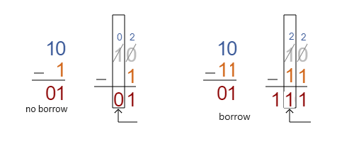
This is means, if A>B, then carry=1, and 0 otherwise. We have to compute the carry bit form right to left and the last carry is the final result. To speed up FHE calculation we could compute 1+ A – B for each bit to make it positive. This example needs only 2 bits to hold the residual. Then we left shift (<<) the carry bit by 2 positions and add the residual. The total number of all outcomes will be 8, which we can use together with the lookup table to output the next carry bit, like in this circuit.

# two numbers are need to presented as  bit arrays
# ---------------------------
# 0 0000 -> 1 less (1+0-1), set the curry bit
# 1 0001 -> 0, equal (1+1-1) or (1+0-0)
# 2 0010 -> 0, greater (1+1-0)
# 3 0100 -> 0 (does not exists)
# carry bit set
# 5 1000 -> 1
# 6 1100 -> 1
# 7 1010 -> 1
# 8 1010 -> 1

from concrete import fhe

table = fhe.LookupTable([1,0,0,0,1,1,1,1])

# result is 1 if less, 0 otherwise
@fhe.compiler({"x": "encrypted", "y": "encrypted"})
def fast_comparision(x, y):
    carry = 0

    # for all the bits
    for i in range(4):
        s = 1 + x[i] - y[i]
        # left shift by 2 (carry << 4)
        carry4 = carry*4 + s
        carry = table[carry4]

    return curry

inputset = [([0,1, 1, 1], [1,0, 1,1])]

circuit = fast_comparision.compile(inputset)

homomorphic_evaluation = circuit.simulate([1,0,1, 0], [1,0,0,0])
print("homomorphic_evaluation =", homomorphic_evaluation)

This method is far more computationally expensive than just using a lookup table, like in the example before this one. However, the memory complexity is far less here, because the lookup table holds only 8 values, resulting in smaller evaluation keys. And yes, as usual, nothing is perfect, as there is a trade off between memory usage vs CPU usage and key sizes, depending on the method you select.

Sorting

Let’s look at the Bubble Sort, which is a simple comparison-based sorting algorithm that repeatedly steps through the list to be sorted, compares each pair of adjacent items, and swaps them if they are in the wrong order. The algorithm gets its name because smaller elements “bubble” to the top of the list (beginning of the array), while larger elements sink to the bottom (end of the array) with each iteration.

from concrete import fhe
import numpy as np

@fhe.compiler({"in_array": "encrypted"})
def bubble_sort(in_array):
    for i in range(len(in_array)):
        for j in range(len(in_array)-1):        
            a = in_array[j]
            b = in_array[j+1]
            flag = a > b
            # if a > b then swap the values
            in_array[j] = flag * b + (1-flag) * a
            in_array[j+1] = flag * a + (1-flag) * b

    return in_array

inputset = [[3,0,0,0]]
circuit = bubble_sort.compile(inputset)

test = [3,2,0,1]
test_clear = test.copy()
test_fhe = test.copy()

clear_evaluation = bubble_sort(test_clear)

#homomorphic_evaluation = circuit.encrypt_run_decrypt(test_fhe)
homomorphic_evaluation = circuit.simulate(test_fhe)

print(test, "=> ", clear_evaluation, "=>", homomorphic_evaluation)

Bubble sort is quite slow [O(n²)] but very memory efficient [O(1)]. For a more CPU efficient algorithm, you can use Merge Sort. It works on the principle of breaking down a list into smaller, more manageable parts (ideally down to individual elements), sorting those parts, and then merging them back together in the correct order.

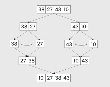
The merge sort has a complexity of O(n log n) , making it one of the most efficient sorting algorithms for large datasets. However, the space complexity is O(n), as it requires additional space proportional to the array size for the temporary merging process.

Dynamic programming

Dynamic programming is a method for solving complex problems by breaking them down into simpler subproblems and solving each of these subproblems just once, storing their solutions. The idea is that if you can solve the smaller subproblems efficiently, you can then use these solutions to tackle the larger problem. Let’s take a Fibonacci numbers as an example.

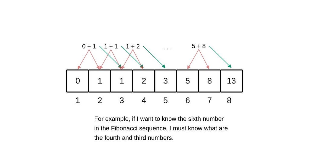
The Fibonacci sequence is a series of numbers where each number is the sum of the two preceding ones, usually starting with 0 and 1. The sequence typically goes 0, 1, 1, 2, 3, 5, 8, 13, and so forth. When solving for the nth Fibonacci number using dynamic programming, the approach can be significantly more efficient than the naive recursive approach by avoiding redundant calculations.

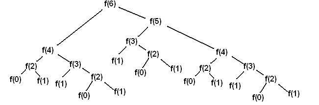
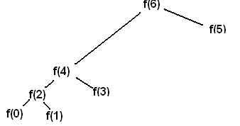
As you can see, to solve for F(6), we need to resolve two subproblems recursively: F(5) and F(4) and so forth. You can note the solutions are overlapping, so the calculation of F(4) happens both on the left and on the right size of the tree. Obviously, we should cache each unique result and thus compute it only once. Then our tree becomes very simple. This approach is called memoization.

However, in the context of Fully Homomorphic Encryption (FHE), memoization cannot typically be used due to the fundamental characteristics and security constraints of FHE. The reason for this is that FHE allows operations to be performed on encrypted data, meaning the actual data values remain concealed throughout the computation.

The other approach for dynamic programming is called tabulation. Tabulation is a bottom-up approach where you solve smaller subproblems first and use their solutions to build solutions to bigger problems. This method is particularly effective for FHE due to its non recursive nature. Tabulation uses a table where on each step, you update the current value. In this example we initialize a table of 6 elements with the base conditions requiring the first element to be 0 and the second element to be 1. The rest of the elements are then initialized to zero: [0,1,0,0,0,0]. Then, we progress from left to right.

This article marks the beginning of a series on Encrypted Data Structures and Algorithms. Up next, I’ll delve into the use of Graphs and Trees, Machine Learning and AI within the realm of Fully Homomorphic Encryption (FHE). Subsequent installments will explore practical applications within financial industry.

—

Ready to Transform Your Coding with Encryption?

Dive deeper into the world of encrypted data structures and algorithms with the open source IDE at FHE-Studio.com. Whether you’re looking to enhance your projects with top-tier security protocols or simply curious about the next generation of data privacy in software development, FHE Studio is a free and open source gateway to the FHE world. Develop, test and share your circuits, and get feedback from peers!

Looking for specialized expertise? Our team at FHE Studio can help you integrate fully homomorphic encryption into your existing projects or develop new encrypted solutions tailored to your needs.

Support us

If you’ve found value in our project, consider supporting us. We’re committed to keeping FHE-Studio open and accessible, and every contribution helps us expand the project.

References

1. FHE-STUDIO.COM, an open source FHE IDE
   2. FHE Studio docs and sources, https://github.com/artifirm
   3. Concrete FHE compiler: https://docs.zama.ai/concrete
   4. Concrete ML is an open-source, privacy-preserving, machine learning framework based on Fully Homomorphic Encryption (FHE). https://docs.zama.ai/concrete-ml
   5. Microsoft SEAL, an open source FHE library https://www.microsoft.com/en-us/research/project/microsoft-seal/
   6. HELib, a FHE library https://github.com/homenc/HElib

Unless otherwise noted, all images are by the author.

---

Coding in Cipher: Encrypted Data Structures and Algorithms was originally published in Towards Data Science on Medium, where people are continuing the conversation by highlighting and responding to this story.

Musings on dominant design and the strategic factors driving the success or failure of generative AI technology in the race for dominance

I. Introduction

The struggle to achieve dominant design within the lifecycle of technology innovation has been the topic of intense study over the last half century. These battles play out within research and development (R&D) labs, in discussions on strategy around commercialization and marketing, and in the media and consumer space, but ultimately in the hearts and minds of the customers who turn the tide of market share and product acceptance through their everyday selections of capability. It is why history remembers VHS and not Betamax, why we type on a QWERTY keyboard, and how the industry changed after the introduction of Google’s search engine or Apple’s iPhone. The emergence of ChatGPT was a signal to the market that we are in the midst of yet another battle for dominant design, this time involving generative AI.

Generative AI, capable of generating new content and performing complex actions, has the potential to revolutionize industries by enhancing creativity, automating tasks, and enhancing customer experiences. As a result, organizations are hastily investing in this ecosystem of capabilities in order to remain relevant and competitive. As business leaders, government agencies, and investors make decisions on technologies within the rapidly evolving field of generative AI, from chips to platforms to models, they should do so with the concept of dominant design in mind and how technologies eventually coalesce around this notion as they mature.

II. The Battle for Dominant Design

The concept of dominant design was first articulated by the Abernathy-Utterback Model[i][ii] in 1975, although the term was not formally coined until twenty years later[iii]. This concept went on to become so foundational that it continues to be taught to MBA students in schools across the country. At its most basic core, this business model describes how a product’s design and manufacturing processes evolve over time through three distinct phases: an initial Fluid Phase characterized by significant experimentation in both product design and process improvement with significant innovation as different approaches are developed and refined to meet market needs, a Transitional Phase where a dominant product design begins to emerge and the market gradually shifts towards increasing product standardization but with substantial process innovation, and a Specific Phase marked by standardization across product and process designs.

This work has since been expanded upon, most prominently by Fernando Suarez, to account for technological dominance dynamics that precede the introduction of a product to the market and can serve as a roadmap to navigate this process. In his integrative framework for technological dominance[iv], Suarez illustrates how product innovation progresses through five phases, covered below.

The Five Phases of Technological Dominance

1. R&D Buildup: Starts as a mix of companies begin conducting applied research related to an emerging technological area. Given the diversity of technological trajectories, the emphasis is on technology and technological talent.
2. Technical Feasibility: The creation of the first working prototype prompts all participating firms to evaluate their current research and their competitive positioning (e.g., continued independent pursuit, partnership/teaming, exit). Competitive dynamics emphasize firm-level factors and technological superiority, as well as regulation if applicable to the market.
3. Creating the Market: The launch of the first commercial product sends a clear signal to the market and irreversibly changes the emphasis from technology to market factors. In this phase, technological differences between products become increasingly less important and strategic maneuvering by firms within the ecosystem becomes most important.
4. The Decisive Battle: The emergence of an early front-runner from among several competitors with sizeable market share signals this phase. Of note, network effects (e.g. ecosystem built around a product) and switching costs in the environment begin to have a stronger impact. In addition, the size of the installed based and complementary assets become critical as mainstream market consumers who seek reliability and trustworthiness over performance and novelty determine the winner(s).
5. Post Dominance: The market adopts one of the alternative designs and becomes the clear dominant technology, supported by a large installed base of users. This serves as a natural defense against new entrants, especially in markets with strong network effects and switching costs. This phase continues until the emergence of a new technological innovation to replace the current one, restarting the cycle.

A firm’s success in navigating these phases to achieve technological dominance is influenced by a number of firm-level factors (e.g., technological superiority, complementary assets, installed user base, strategic maneuvering) and environmental factors (e.g., industry regulation, network effects, switching costs, appropriability regime, market characteristics). Each of these factors have differing levels of importance in a given stage, with actions occurring too early or too late within the process having muted or unintended effects. Work has also been conducted to consider how sequential decisions on three key aspects (i.e., the market, the technology, complementary assets) can help determine success or failure in the battle for dominance[v]. The first decision relates to the market and the decisions needed to correctly visualize the market to drive the actions to achieve a superior installed user base. The second decision relates to whether the market standard is government or market driven and includes a consideration of a strategy of proprietary control vs one of openness. The third and final decision relates to the strategy to cultivate access to the complementary assets required to be competitive in a mainstream market.

An additional factor that one must consider is technological path dependency and the impact of previous outcomes (e.g., the cloud wars, AI chip investments) on the course of future events. Modern, complex technologies often operate within a regime of increasing returns to adoption, in that the more a technology is adopted, the more beneficial and entrenched it becomes[vi]. Within this context, small historical events can have a strong influence in which technology ultimately becomes dominant, despite the potential advantages of competing technologies. This results from several reinforcing mechanisms such as learning effects, coordination effects, and adaptive expectations that make switching to another technology costly and complex. Moreover, the transition of enterprise-scale generative AI from R&D to commercialized product with business and operational value is intertwined with cloud infrastructure dominance[vii]. This is necessitated by the need for a common set of capabilities coupled with large scale computational resources. To provide such capabilities, hyperscalers have seamlessly integrated cloud infrastructure, models, and applications into the cloud AI stack — accelerating the creation of complementary assets. It is through the lens of these considerations that the developments in generative AI are examined.

III. ChatGPT: The Shot Heard Around the World

The emergence of ChatGPT in November 2022 sent a clear signal that large language models (LLMs) had practical, commercial application on a broad scale. Within weeks, the term generative AI was known across generations of users, technical and non-technical alike. Even more profound was the realization by other participants in the market that they needed to either initiate or significantly accelerate their own efforts to deliver generative AI capability. This marked the transition from Phase 2: Technical Feasibility to Phase 3: Creating the Market. From there, the race was on.

In fairly quick succession, major technology providers began releasing their own generative AI platforms and associated models (e.g., Meta AI — February 2023, AWS Bedrock — April 2023, Palantir Artificial Intelligence Platform — April 2023, Google Vertex AI — June 2023, IBM WatsonX.ai — July 2023). Where technology and technological talent were of greatest importance in proving technical feasibility, this has given way to strategic maneuvering as firms work to position themselves for growth with a focus on building up the installed user base, developing complementary assets and ecosystems, and enhancing networking effects. This is leading to the current period of rapid expansion of strategic partnerships across hyperscaler ecosystems and with key AI providers as organizations seek to form the alliances that will help them weather the decisive battle for dominance. We are also seeing hyperscalers leverage their existing cloud infrastructure assets to pull their generative AI assets through regulatory hurdles at an accelerated pace in niche markets with little to no competition.

As this plays out, organizations should remain cognizant of various risks. For one, AI companies that invest in alternative approaches that do not become the dominant design may find themselves at a disadvantage. Consequently, adapting to or adopting the dominant design could require significant shifts in strategy, development, and investment beyond current sunk costs. Additionally, competition will continue to increase as the generative AI market’s potential becomes more evident, increasing pressure on all market participants and eventually leading to consolidation and exits. Lastly, the pervasiveness of AI is leading world governments and institutions to begin updating regulatory frameworks to promote security and the responsible deployment of AI. This is introducing added uncertainty as organizations may face new compliance requirements which can be resource-intensive to implement. In markets with heavy regulation, this may prove a barrier to being able to even provide generative AI tools, if those tools do not meet basic requirements.

However, this current period is not without opportunities. As the market begins to identify front runners in the battle for dominant design, organizations that can quickly align with the dominant design(s) or innovate within those frameworks are better positioned to capture significant market share. Also, even as the market begins to standardize around a dominant design, new niches can emerge within the AI field. If identified early and capitalized on, companies can establish a strong presence and enjoy first-mover advantages.

IV. Indicators of Technological Dominance

As the current race for dominant design continues, one can expect to observe the emergence of several indicators that can help predict which technologies or companies might establish market leadership and set the standard for generative AI applications within the current evolving landscape.

1. Leadership Emergence in Market Share: AI companies and platforms able to secure a large installed user base with respect to the market may wield a front-runner status. This could be evidenced by widespread adoption of their platforms, increased user engagement, growing sales figures, or clients within a specific market. An early lead in market share can be a significant indicator of potential dominance.
2. Development and Expansion of Ecosystems: Observation of the ecosystems surrounding different generative AI technologies may identify strong, expansive ecosystems, with complementary technologies that can enhance the value of a generative AI platform. The strength of these ecosystems often plays a crucial role in the adoption and long-term viability of a technology.
3. Switching Costs: Switching costs associated with moving away from one generative AI platform to another can deter users from moving to competing technologies, thereby strengthening the position of the current leader. These could include data integration issues, the need for retraining machine learning models, or contractual and business dependencies.
4. Size of the Installed Base: A large installed base of users and solutions improves network effects and provides a critical mass that can attract further users due to perceived reliability, the support ecosystem, interoperability, and learning effects. This also activates the bandwagon effect, attracting risk-adverse users who may otherwise avoid technology adoption[v].
5. Reliability and Trustworthiness: Gauge market sentiment regarding the reliability and trustworthiness of different generative AI technologies. Market consumers often favor reliability and trustworthiness over performance and novelty. Brands that are perceived as reliable and receive positive feedback for user support and robustness are likely to gain a competitive edge.
6. Innovations and Improvements: Company investments in innovations within their generative AI offerings may indicate dominance. While the market may lean towards established, reliable technologies, continuous improvement and adaptation to user needs will be crucial for continued competitiveness.
7. Regulatory Compliance and Ethical Standards: Companies and organizations that lead in developing ethically aligned AI in compliance with increasing regulations could be favored by the market, particularly in heavily regulated industries. This is especially important within the Federal market, where network accreditations and unique security requirements play an outsized role in the technologies that can be leveraged for operational value.

By monitoring these indicators, organizations can gain insights into which technologies might emerge as leaders in the generative AI space during the decisive battle phase. Understanding these dynamics is crucial when making investment, development, or implementation decisions on generative AI technologies.

V. Conclusion

Establishment of a dominant design in generative AI is an important step for market stability and industry-wide standardization, which will lead to increased market adoption and reduced uncertainty among businesses and consumers alike. Companies that can influence or adapt to emerging dominant designs will secure competitive advantages, establishing themselves as market leaders in the new technological paradigm. However, selecting a product ecosystem that ultimately does not become the standard will lead to diminishing market share and exact switching costs upon the firms that will now need to transition to the dominant design.

As the industry moves from the fluid to the specific, flowing with increasing viscosity toward a dominant design, strategic foresight and agility become more critical than ever if organizations intend to create value from and deliver impact with technology. The necessity to anticipate future trends and swiftly adapt to evolving technological landscapes means that organizations must stay vigilant and flexible, ready to pivot their strategies in response to new developments in AI technology and shifts in consumer demands. Businesses that can envision the trajectory of technological change and proactively respond to it will not only endure but also stand out as pioneers in the new era of digital transformation. Those that cannot, will be relegated to the annals of history.

All views expressed in this article are the personal views of the author.

References:

[i] J. Utterback, W. Abernathy, “A dynamic model of process and product innovation,” Omega, Vol. 3, Issue 6. 1975

[ii] W. Abernathy, J. Utterback, “Patterns on Innovation”, Technology Review, Vol. 80, Issue 7. 1978

[iii] F. Suárez, J. Utterback, “Dominant Designs and the Survival of Firms,” Strategic Management Journal, Vol. 16, №6. 1995, 415–430

[iv] F. Suárez, “Battles for technological dominance: an integrative framework,” Research Policy, Vol. 33, 2004, 271–286

[v] E. Fernández, S. Valle, “Battle for dominant design: A decision-making model,” European Research on Management and Business Economics, Vol. 25, Issue 2. 2019, 72–78

[vi] W.B. Arthur, “Competing Technologies, Increasing Returns, and Lock-In by Historical Events,” The Economic Journal, Vol. 99, №394, 1989, 116–131

[vii] F. van der Vlist, A. Helmond, F. Ferrari, “Big AI: Cloud infrastructure dependence and the industrialisation of artificial intelligence,” Big Data and Society, January-March: I-16, 2024, 1, 2, 5, 6

---

The Path to Dominant Design in Generative AI was originally published in Towards Data Science on Medium, where people are continuing the conversation by highlighting and responding to this story.

Competitions are more valuable than other components

Kaggle is a platform for users to gain hands-on experience on practical data science and machine learning. It has 4 different progression components, namely Competitions, Datasets, Notebooks and Discussions. No prior experience in data science is necessary to get yourself started in using this platform and learn

My background: I did my first project on Kaggle as part of a Machine Learning course in my Bachelor’s curriculum (Math + Comp Sci) in early 2023. Since then I have been hooked to this platform as a favorite pastime. I have taken part in 20 competitions to date. I had no work/internship experience as a data scientist prior to starting Kaggle.

In one year, I have made (I believe) significant progress in my Kaggle journey, including winning 2 gold competition medals, one of which I won 1st place and rising to the top 116 in the Competitions category, while barely missing a day of activity.

My Kaggle Profile

Now, let’s dive into 3 key learnings from my Kaggle journey to date.

1. Your team cannot solely rely on public notebooks to succeed in Competitions

A standard Kaggle competition only awards Gold medals to the top 10 + floor(NumTeams / 500) teams! For example, in a competition with 2500 teams, only 15 teams win gold. This is mandatory for one to progress to the Master tier in competitions, and you need five (including one solo) to progress to the Grandmaster tier.

It is very unlikely that your team could just briefly modify public work (such as ensembling public notebooks) and earn a spot in the gold zone. Your team will be competing against top-notch data scientists and grandmasters who have lots of creative ideas to approach the problem.

Briefly modifying public work is something even beginners to ML can do and it is unlikely your team’s solution stands out using this. Most likely, a small enhancement of a public notebook gets a bronze medal, or if lucky, a silver medal.

In the 2 competitions which my team won gold:

• 1/2048 (Champion) PII Detection: We used a wide variety of Deberta architectures and postprocessing strategies, most of which are not shared in the public forums. No public models were used in our final ensemble
• 14/4436 Optiver — Trading At The Close: We used online training to make sure the model is fitted with the latest data before making the prediction. It was not easy to write an online training pipeline that worked on the private LB, and such an idea was not shared in the public forums, as far as I know. We did not use the popular public training approach as we felt it was overfitting to the train data, despite its great public LB score

In contrast, here is a competition in which my team won bronze:

• 185/2664 LLM Science Exam: We briefly modified a public training pipeline and a public inference pipeline, such as changing the embedding model, hyperparameters and ensembling. There was no creative ideas in our final solution

Summary: In my opinion, it is better to spend more time analyzing the baseline, and research to think of enhancements. It may be a good idea to start with a small model (deberta-v3-xsmall for example) to evaluate ideas quickly. Aim to establish a robust cross-validation strategy from the very beginning.

2. You learn much more from the Competitions category compared to Datasets/Notebooks/Discussions

Some of the real-world skills I learnt

• I was the team leader for most of the competitions I participated in, including both of them which my team won the gold medal. It has drastically improved my communication and leadership skills.
• Collaborating with other data scientists/engineers from different countries and timezones, and learning good practices from them
• Using Wandb to track and log experiments
• Customizing architectures of transformer models
• Generating use-case specific synthetic datasets using LLMs
• How to model a real-world use case in a data science perspective
• Writing clean code that is easily understandable
• How to utilize multi-GPU training
• Better time management
• Evaluating and mitigating model mistakes

In contrast, it is much easier to progress in datasets/notebooks/discussions without learning much about data science. In discussions, a user can earn gold discussion medals by posting his/her accomplishments on the Kaggle forum. I doubt I would learn most of the skills above without doing competitions. In my opinion, progress on datasets/notebooks/discussions does not necessarily tell that one is passionate about data science.

3. Playground Competitions is a great way to start for beginners

The playground series simulate the featured competitions, except that it is more beginner-friendly and do not award medals/prizes. In playgrounds, you make predictions on a tabular dataset, which allows you to learn the basics of coding an ML pipeline. Plenty of notebooks are shared in playgrounds, both tabular and NN (neural network) approaches, so if you are stuck, those public notebooks are a good reference.

Each playground series competition is about 1 month long.

Based on my experience, the playground competitions taught me:

• How to build a robust cross-validation strategy and not overfit the public LB
• How to select submissions for evaluation
• How to perform feature engineering and feature selection
• How to style a Jupyter Notebook
• (More on the data engineering side of things) How to use Polars. This is a much faster dataframe library than Pandas and is better suited for big data use cases

In conclusion, I feel the most rewarding part from doing Kaggle is the hands-on experience in competitions and the opportunity to collaborate with data professionals from around the globe. I get to solve a wide variety of problems ranging from tabular to more advanced NLP tasks. Looking forward to more as I continue to improve myself in the field of data science!

---

One Year of Consistent Kaggling: What Did It Teach Me? was originally published in Towards Data Science on Medium, where people are continuing the conversation by highlighting and responding to this story.

Crafting new questions for exams and quizzes can be tedious and time-consuming for educators. The time required varies based on factors like subject matter, question types, experience level, and class level. Multiple-choice questions require substantial time to generate quality distractors and ensure a single unambiguous answer, and composing effective true-false questions demands careful effort to […]

ONNX is an open source machine learning (ML) framework that provides interoperability across a wide range of frameworks, operating systems, and hardware platforms. ONNX Runtime is the runtime engine used for model inference and training with ONNX. AWS Graviton3 processors are optimized for ML workloads, including support for bfloat16, Scalable Vector Extension (SVE), and Matrix […]

Amazon Ads helps advertisers and brands achieve their business goals by developing innovative solutions that reach millions of Amazon customers at every stage of their journey. At Amazon Ads, we believe that what makes advertising effective is delivering relevant ads in the right context and at the right moment within the consumer buying journey. With that […]