Strategies and Insights from Both Sides of the Interview Table
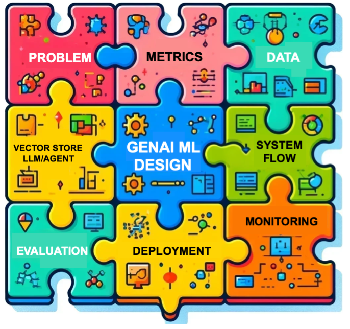
Mastering GenAI ML System Design Interview: Principles & Solution Outline
Mastering GenAI ML System Design Interview: Principles & Solution Outline

Strategies and Insights from Both Sides of the Interview Table

How to detect and fix any type of error in a directed acyclic graph so that it is a valid representation of the underlying data
Originally appeared here:
Causal Validation: A Unified Theory of Everything
Go Here to Read this Fast! Causal Validation: A Unified Theory of Everything


You don’t need to know math to learn this powerful statistical test. And if you’re going to learn only one statistical test, it should be…
Originally appeared here:
The Colorful Power of Permutation Tests
Go Here to Read this Fast! The Colorful Power of Permutation Tests

Originally appeared here:
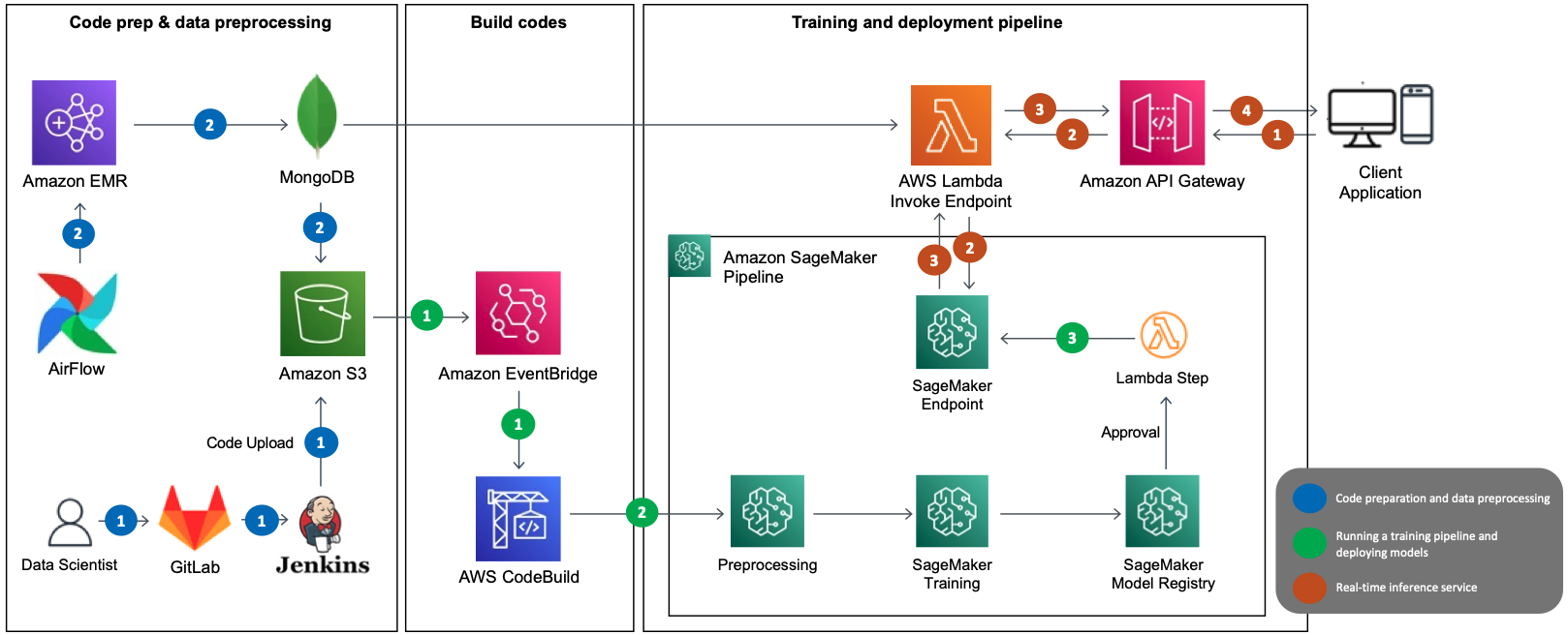
How LotteON built a personalized recommendation system using Amazon SageMaker and MLOps

The first two blogs in this series described how different architectural motifs ranging from graph neural networks to sparse transformers addressed the challenges of “long-form” video representation learning. We showed how explicit graph based methods can aggregate 5-10X larger temporal context, but they were two-stage methods. Next, we explored how we can make memory and compute efficient end-to-end learnable models based on transformers and aggregate over 2X larger temporal context.
In this blog, I’ll take you to our latest and greatest explorations, especially for egocentric video understanding. As you can imagine, an egocentric or first-person video (captured usually by head-mounted cameras) is most likely coming from an always-ON camera, meaning the videos are really really long, with a lot of irrelevant visual information, specially when the camera wearer move their heads. And, this happens a lot of times with head mounted cameras. A proper analysis of such first-person videos can enable a detailed understanding of how humans interact with the environment, how they manipulate objects, and, ultimately, what are their goals and intentions. Typical applications of egocentric vision systems require algorithms able to represent and process video over temporal spans that last in the order of minutes or hours. Examples of such applications are action anticipation, video summarization, and episodic memory retrieval.
We present Egocentric Action Scene Graphs (EASGs), a new representation for long-form understanding of egocentric videos. EASGs extend standard manually-annotated representations of egocentric videos, such as verb-noun action labels, by providing a temporally evolving graph-based description of the actions performed by the camera wearer. The description also includes interacted objects, their relationships, and how actions unfold in time. Through a novel annotation procedure, we extend the Ego4D dataset adding manually labeled Egocentric Action Scene Graphs which offer a rich set of annotations for long-from egocentric video understanding.
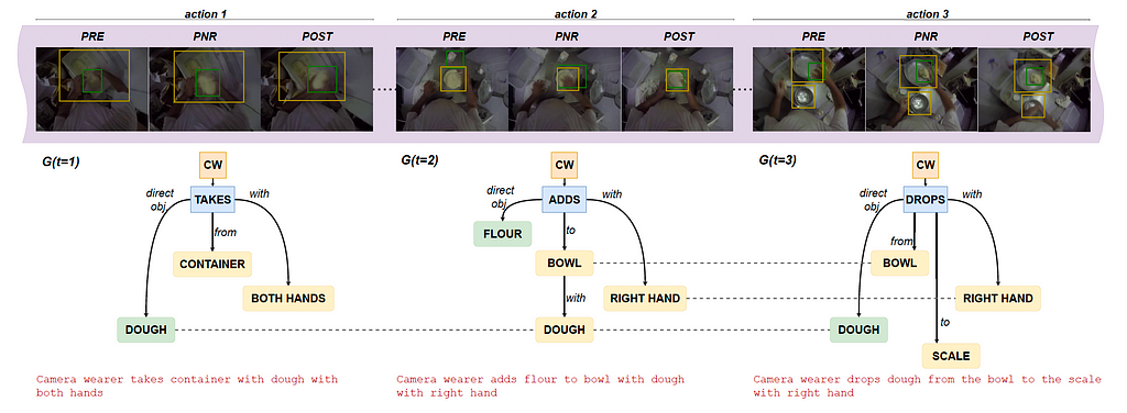
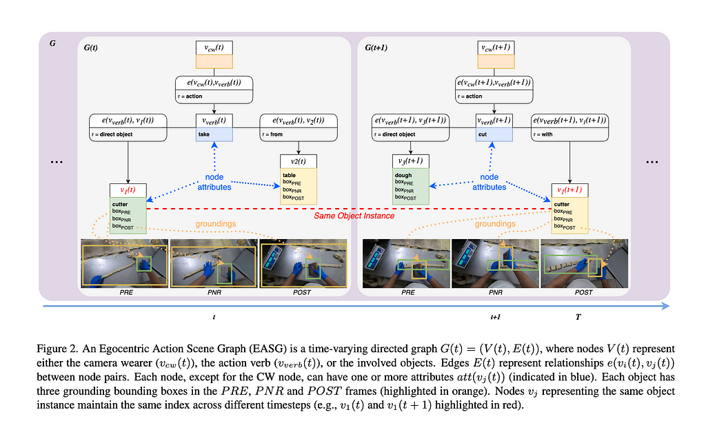
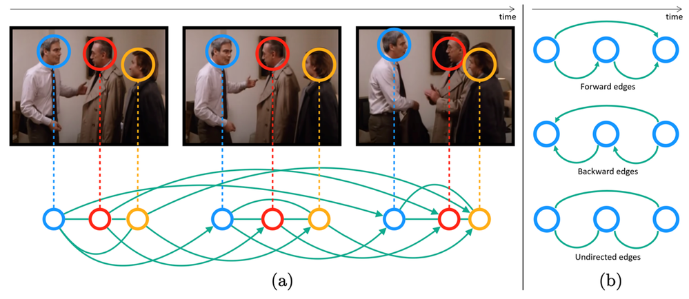
EASGs provide annotations for a video clip in the form of a dynamic graph. We formalize an EASG as a time-varying directed graph G(t) = (V (t), E(t)), where V (t) is the set of nodes at time t and E(t) is the set of edges between such nodes (Figure 2). Each temporal realization of the graph G(t) corresponds to an egocentric action spanning over a set of three frames defined as in [Ego4D]: the precondition (PRE), the point of no return (PNR) and the postcondition (POST) frames. The graph G(t) is hence effectively associated to three frames: F(t) = {PREₜ, PNRₜ, POSTₜ}, as shown in figure 1 below.
Figure 2 shows an example of an annotated graph in details.
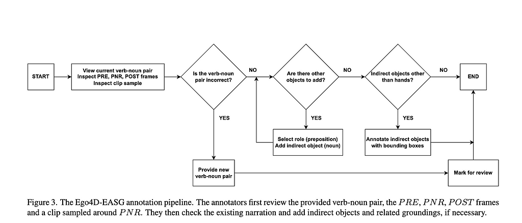
We obtain an initial EASG leveraging existing annotations from Ego4D, with initialization and refinement procedure. e.g. we begin with adding the camera wearer node, verb node and and the default action edge from camera wearer node to the verb node. The annotation pipeline is shown in figure 3 below.
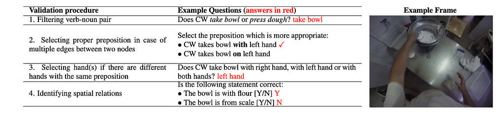
Next, we do the graph refinement via inputs from 3 annotators. The validation stage aggregates the data received from three annotators and ensures the quality of the final annotations as shown below.
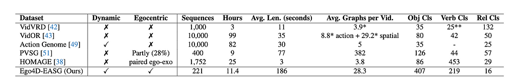
As it can be noted, the EASG dataset is unique in its labels. And, in the table below you can see how this new dataset compares with other video datasets with visual relations, in terms of labels and size.
After the creation of this unique dataset, we will now describe different tasks that are evaluated on this dataset. The first set of tasks is about generating action scene graphs which stems from the image scene graph generation literature. In other words we aim to learn EASG representations in a supervised way and measure its performance in standard Recall metrics used in scene graph literature. We devise baselines and compare the EASG generation performance of different baselines on this dataset.

We show the potential of the EASG representation in the downstream tasks of action anticipation and activity summarization. Both tasks require to perform long-form reasoning over the egocentric video, processing long video sequences spanning over different time-steps. Following recent results showing the flexibility of Large Language Models (LLMs) as symbolic reasoning machines, we perform these experiments with LLMs accessed via the OpenAI API. The experiments aim to examine the expressive power of the EASG representation and its usefulness for downstream applications. We show that EASG offers an expressive way of modeling long-form activities, in comparison with the gold-standard verb-noun action encoding, extensively adopted in egocentric video community.
Action anticipation with EASGs:
For the action anticipation task, we use the GPT3 text-davinci-003 model. We prompt the model to predict the future action from a sequence of length T ∈ {5, 20}. We compare two types of representations — EASG and sequences of verb-noun pairs. Below table shows the results of this experiment.

Even short EASG sequences (T =5) tend to outperform long V-N sequences (T = 20), highlighting the higher representation power of EASG, when compared to standard verb-noun representations. EASG representations achieve the best results for long sequences (T = 20).
Long-form activity summarization with EASGs:
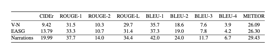
We select a subset of 147 Ego4D-EASG clips containing human-annotated summaries describing the activities performed within the clip in 1–2 sentences from Ego4D. We construct three types of input sequences: sequences of graphs S-EASG = [G(1), G(2), …, G(Tmax)], sequences of verb-noun pairs svn = [s-vn(1), s-vn(2), …, s-vn(Tmax)], and sequences of original Ego4D narrations, matched with the EASG sequence. This last input is reported for reference, as we expect summarization from narrations to bring the best performance, given the natural bias of language models towards this representation.
Results reported in the below table indicate strong improvement in CIDEr score over the sequence of verb-noun inputs, showing that models which process EASG inputs capturing detailed object action relationships, will generate more specific, informative sentences that align well with reference descriptions.
We believe that these contributions mark a step forward in long-form egocentric video understanding.
Highlights:
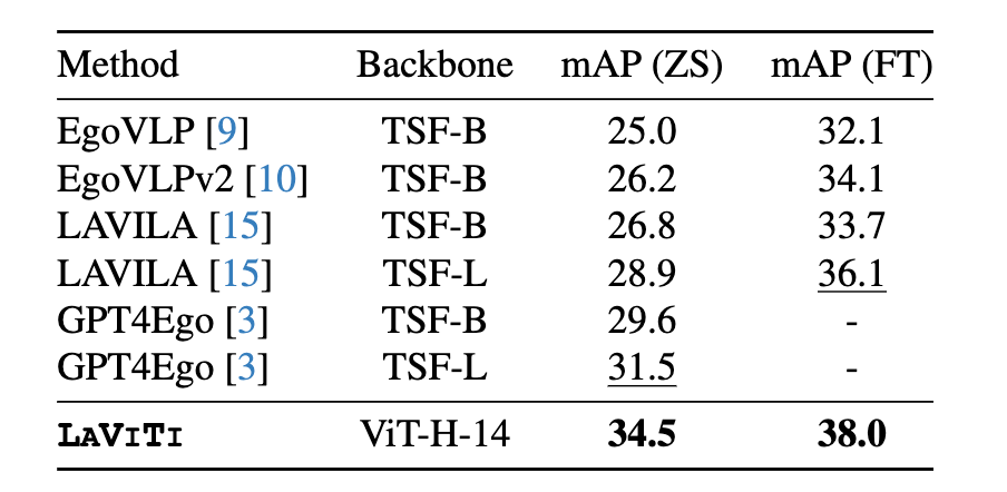
In recent years, egocentric video-language pre-training (VLP) has been adopted significantly in academia and in industry. A line of works such as EgoVLP, EgoVLPv2 learn transferable spatial-temporal representations from large-scale video-text datasets. Recently, LaViLa showed that VLP can benefit from the dense narrations generated by Large Language Models (LLMs). However, all such methods do hit the memory and compute bottleneck while processing video sequences, each consisting of a small number of frames (e.g. 8 or 16 frame models), leading to limited temporal context aggregation capability. On the contrary, our model, called LAVITI, is equipped with long-form reasoning capability (1,000 frames vs 16 frames) and is not limited to a small number of input frames.
In this ongoing work, we devised a novel approach to learning language, video, and temporal representations in long-form videos via contrastive learning. Unlike existing methods, this new approach aims to align language, video, and temporal features by extracting meaningful moments in untrimmed videos by formulating it as a direct set prediction problem. LAVITI outperforms existing state-of-the-art methods by a significant margin on egocentric action recognition, yet is trainable on memory and compute-bound systems. Our method can be trained on the Ego4D dataset with only 8 NVIDIA RTX-3090 GPUs in a day.
As our model is capable of long-form video understanding with explicit temporal alignment, the Ego4D Natural Language Query (NLQ) task is a natural fit with the pre-training targets. We can directly predict intervals which are aligned with language query given a video; therefore, LAVITI can
perform the NLQ task under the zero-shot setting (without modifications of the architecture and re-training on NLQ annotations).
In the near future, we plan on assessing its potential to learn improved representations for episodic memory tasks including NLQ and Moment Query (MQ). To summarize, we are leveraging existing foundation models (essentially “short-term”) for creating “long-form” reasoning module aiming at 20X-50X larger context aggregation.
Highlights:
We devised exciting new ways for egocentric video understanding. Our contributions are manifold.
Watch out for more exciting results with this new paradigm of “long-form” video representation learning!
Long-form video representation learning (Part 3: Long-form egocentric video representation… was originally published in Towards Data Science on Medium, where people are continuing the conversation by highlighting and responding to this story.
Originally appeared here:
Long-form video representation learning (Part 3: Long-form egocentric video representation…

The first blog in this series was about learning explicit sparse graph-based video representation methods for “long-form” video representation learning. They are effective methods; however, they were not end-to-end trainable. We needed to rely on other CNN or transformer-based feature extractors to generate the initial node embeddings. In this blog, our focus is to devising an end-to-end methods using transformers, but with the same goal of “long-form” reasoning.
As an end-to-end learnable architecture, we started exploring transformers. The first question we needed an answer for is that do video-text transformers learn to model temporal relationships across frames? We oberved that despite their immense capacity and the abundance of multimodal training data, recent video models show strong tendency towards frame-based spatial representations, while temporal reasoning remains largely unsolved. For example, if we shuffle the order of video frames in the input to the video models, the output do not change much!
Upon a closer investigation, we identify a few key challenges to incorporating multi-frame reasoning in video-language models. First, limited model size implies a trade-off between spatial and temporal learning (a classic example being 2D/3D convolutions in video CNNs). For any given dataset, optimal performance requires a careful balance between the two. Second, long-term video models typically have larger model sizes and are more prone to overfitting. Hence, for long-form video models, it becomes more important to carefully allocate parameters and control model growth. Finally, even if extending the clip length improves the results, it is subject to diminishing returns since the amount of information provided by a video clip does not grow linearly with its sampling rate. If the model size is not controlled, the compute increase may not justify the gains in accuracy. This is critical for transformer-based architectures, since self-attention mechanisms have a quadratic memory and time cost with respect to input length.
In summary, model complexity should be adjusted adaptively, depending on the input videos, to achieve the best trade-off between spatial representation, temporal representation, overfitting potential, and complexity. Since existing video-text models lack this ability, they either attain a suboptimal balance between spatial and temporal modeling, or do not learn meaningful temporal representations at all.
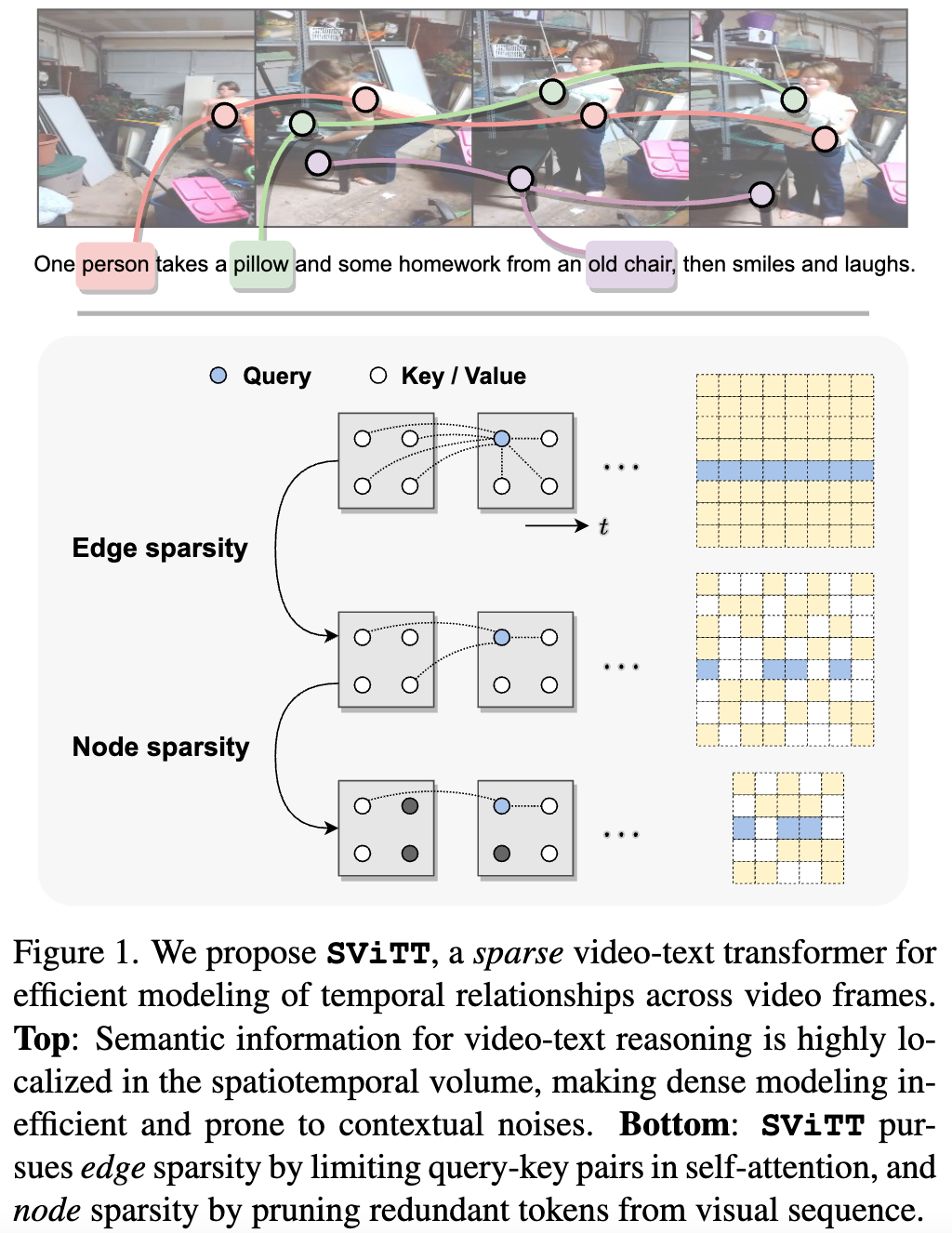
We argue that video-text models should learn to allocate modeling resources to the video data. Rather than uniformly extending the model to longer clips, the allocation of these resources to the relevant spatio-temporal locations of the video is crucial for efficient learning from long clips. For transformer models, this allocation is naturally performed by pruning redundant attention connections. We then accomplish these goals by exploring transformer sparsification techniques. This motivates the introduction of a Sparse Video-Text Transformer SViTT inspired by graph models. As illustrated in Figure 1, SViTT treats video tokens as graph vertices, and self-attention patterns as edges that connect them.
We design SViTT to pursue sparsity for both: Node sparsity reduces to identifying informative tokens (e.g., corresponding to moving objects or person in the foreground) and pruning background feature embeddings; edge sparsity aims at reducing query-key pairs in attention module while maintaining its global reasoning capability. And, node sparsity reduces to identifying informative tokens (e.g., corresponding to moving objects or person in the foreground) and pruning background feature embeddings. To address the diminishing returns for longer input clips, we propose to train SViTT with temporal sparse expansion, a curriculum learning strategy that increases clip length and model sparsity, in sync, at each training stage.
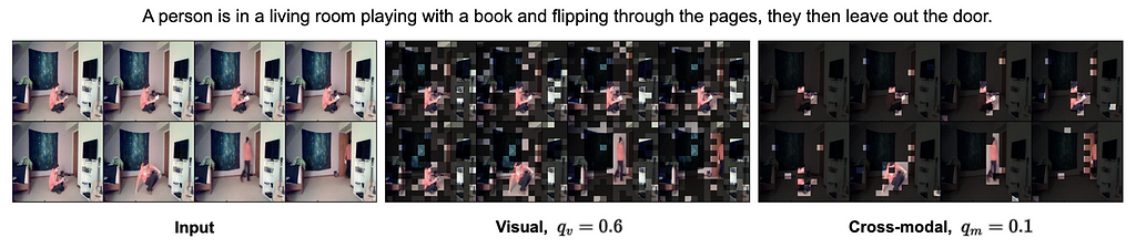
SViTT is evaluated on diverse video-text benchmarks from video retrieval to question answering, comparing to prior art and our own dense modeling baselines. First, we perform a series of ablation studies to understand the benefit of sparse modeling in transformers. Interestingly, we find that both nodes (tokens) and edges (attention) can be pruned drastically at inference, with a small impact on test performance. In fact, token selection using cross-modal attention improves retrieval results by 1% without re-training. Figure 2 shows that SViTT isolates informative regions from background patches to facilitate efficient temporal reasoning.
We next perform full pre-training with the sparse models and evaluate their downstream performance. We observe that SViTT scales well to longer input clips, where the accuracy of dense transformers drop due to optimization difficulties. On all video-text benchmarks, SViTT reports comparable or better performance than their dense counterparts with lower computational cost, outperforming prior arts including those trained with additional image-text corpora.
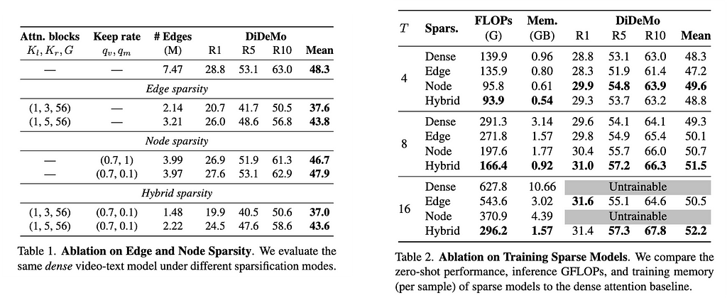
We can see from the above tables, with sparsification, immediate temporal context aggregation could be made 2X longer (table 2). Also see how sparsification maintains the final task accuracies (table 1), rather improves them.
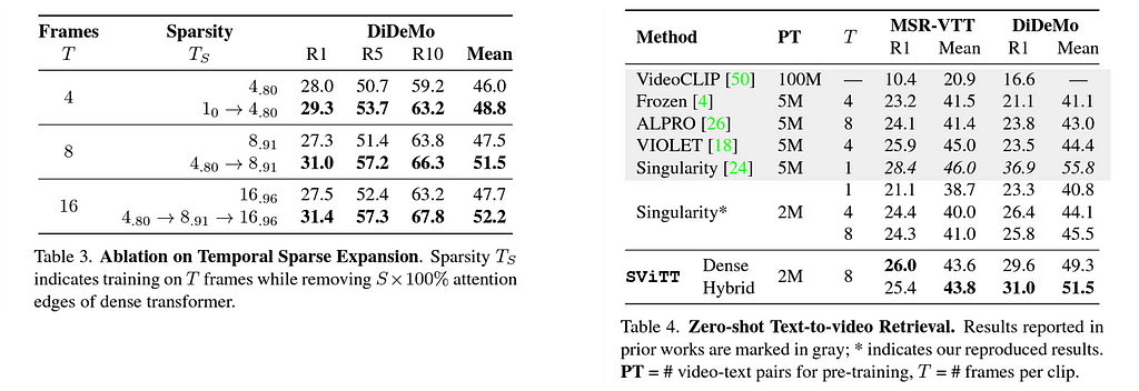
In the above table, we show how our proposed training paradigm helps improve task performance with respect to the different levels of sparsity. In table 4, you can see the zero-shot performance on text-to-video retrieval task on two standard benchmarks.
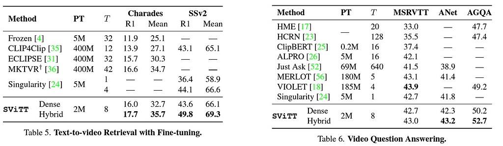
Finally, we show the results on different benchmarks on multimodal retrieval and video question-answering. SViTT outperforms all existing methods, and even required less number of pre-training pairs.
More details on SViTT can be found here . To summarize, Compared to original transformers, SViTT is 6–7 times more efficient, capable of 2X more context aggregation. Pre-training with SViTT improves accuracy SoTA on 5 benchmarks : retrieval, VideoQ&A.
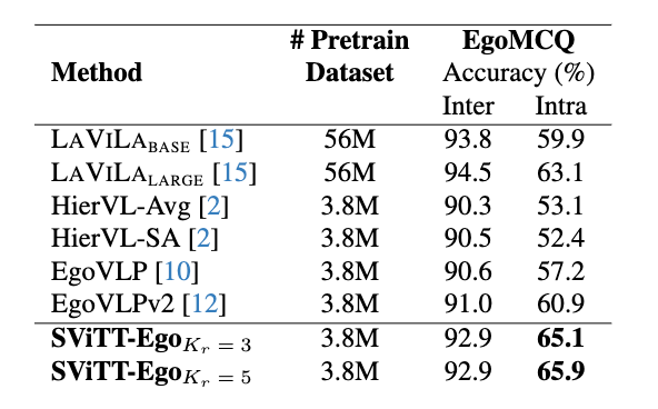
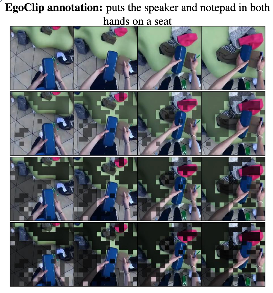
Pretraining egocentric vision-language models has become essential to improving downstream egocentric video-text tasks. These egocentric foundation models commonly use the transformer architecture. The memory footprint of these models during pretraining can be substantial. Therefore, we pre-train our own sparse video-text transformer model, SViTT-Ego, the first sparse egocentric video-text transformer model integrating edge and node sparsification. We pretrain on the EgoClip dataset and incorporate the egocentric-friendly objective EgoNCE, instead of the frequently used InfoNCE. Most notably, SViTT-Ego, obtains a 2.8% gain on EgoMCQ (intra-video) accuracy compared to the current SOTA, with no additional data augmentation techniques other than standard image augmentations, yet pre-trainable on memory-limited devices. One such visual example is shown below. We are preparing to participate in the EgoVis workshop at CVPR with our SViTT-ego.

We propose, SViTT, a video-text architecture that unifies edge and node sparsity; We show its temporal modeling efficacy on video-language tasks. Compared to original transformers, SViTT is 6–7 times more efficient, capable of 2X more context aggregation. Pre-training with SViTT improves accuracy over SoTA on 5 benchmarks : retrieval, VideoQ&A. Our video-text sparse transformer work was first published at CVPR 2023.
Next, we show how we are leveraging such sparse transformer for egocentric video understanding applications. We show our SViTT-Ego (built atop SViTT) outperforms dense transformer baselines on the EgoMCQ task with significantly lower peak memory and compute requirements thanks to the inherent sparsity. This shows that sparse architectures such as SViTT-Ego is a potential foundation model choice, especially for pretraining on memory-bound devices. Watch out for exciting news in the near future!
Long-form video representation learning (Part 2: Video as sparse transformers) was originally published in Towards Data Science on Medium, where people are continuing the conversation by highlighting and responding to this story.
Originally appeared here:
Long-form video representation learning (Part 2: Video as sparse transformers)

Existing video architectures tend to hit computation or memory bottlenecks after processing only a few seconds of the video content. So, how do we enable accurate and efficient long-form visual understanding? An important first step is to have a model that practically runs on long videos. To that end, we explore novel video representations methods that are equipped with long-form reasoning capability.
As we saw the huge leap of success of image-based understanding tasks with deep learning models such as convolutions or transformers, the next step naturally became going beyond still images and exploring video understanding. Developing video understanding models require two equally important focus areas. First is a large scale video dataset and the second is the learnable backbone for extracting video features efficiently. Creating finer-grained and consistent annotations for a dynamic signal such as a video is not trivial even with the best intention from both the system designer as well as the annotators. Naturally, the large video datasets that were created, took the relatively easier approach of annotating at the whole video level. About the second focus area, again it was natural to extend image-based models (such as CNN or transformers) for video understanding since videos are perceived as a collection of video frames each of which is identical in size and shape of an image. Researchers made their models that use sampled frames as inputs as opposed to all the video frames for obvious memory budget. To put things into perspective, when analyzing a 5-minute video clip at 30 frames/second, we need to process a bundle of 9,000 video frames. Neither CNN nor Transformers can operate on a sequence of 9,000 frames as a whole if it involves dense computations at the level of 16×16 rectangular patches extracted from each video frame. Thus most models operate in the following way. They take a short video clip as an input, do prediction, followed by temporal smoothing as opposed to the ideal scenario where we want the model to look at the video in its entirety.
Now comes this question. If we need to know whether a video is of type ‘swimming’ vs ‘tennis’, do we really need to analyze a minute-worth content? The answer is most certainly NO. In other words, the models optimized for video recognition, most likely learned to look at background and other spatial context information instead of learning to reason over what is actually happening in a ‘long’ video. We can term this phenomenon as learning the spatial shortcut. These models were good for video recognition tasks in general. Can you guess how do these models generalize for other tasks that require actual temporal reasoning such as action forecasting, video question-answering, and recently proposed episodic memory tasks? Since they weren’t trained for doing temporal reasoning, they turned out not quite good for those applications.
So we understand that datasets / annotations prevented most video models from learning to reason over time and sequence of actions. Gradually, researchers realized this problem and started coming up with different benchmarks addressing long-form reasoning. However, one problem still persisted which is mostly memory-bound i.e. how do we even make the first practical stride where a model can take a long-video as input as opposed to a sequence of short-clips processed one after another. To address that, we propose a novel video representation method based on Spatio-Temporal Graphs Learning (SPELL) to equip the model with long-form reasoning capability.
Let G = (V, E) be a graph with the node set V and edge set E. For domains such as social networks, citation networks, and molecular structure, the V and E are available to the system, and we say the graph is given as an input to the learnable models. Now, let’s consider the simplest possible case in a video where each of the video frame is considered a node leading to the formation of V. However, it is not clear whether and how node t1 (frame at time=t1) and node t2 (frame at time=t2) are connected. Thus, the set of edges, E, is not provided. Without E, the topology of the graph is not complete, resulting into unavailability of the “ground truth” graphs. One of the most important challenges remains how to convert a video to a graph. This graph can be considered as a latent graph since there is no such labeled (or “ground truth”) graph available in the dataset.
When a video is modeled as a temporal graph, many video understanding problems can be formulated as either node classification or graph classification problems. We utilize a SPELL framework for tasks such as Action Boundary Detection, Temporal Action Segmentation, Video summarization / highlight reels detection.
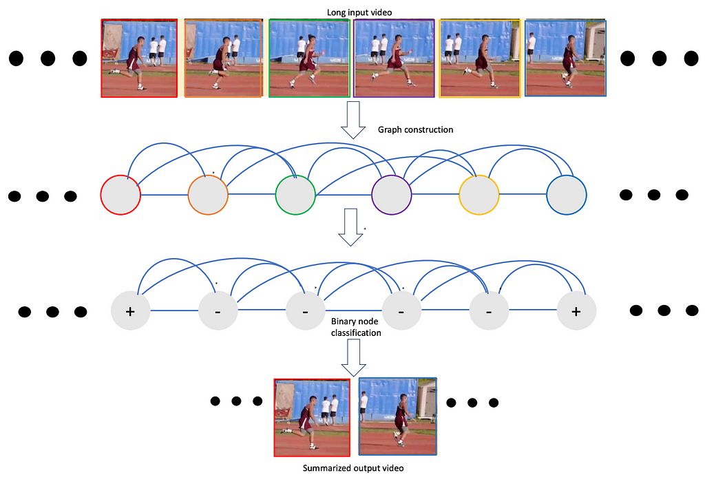
Here we present such a framework, namely VideoSAGE which stands for Video Summarization with Graph Representation Learning. We leverage the video as a temporal graph approach for video highlights reel creation using this framework. First, we convert an input video to a graph where nodes correspond to each of the video frames. Then, we impose sparsity on the graph by connecting only those pairs of nodes that are within a specified temporal distance. We then formulate the video summarization task as a binary node classification problem, precisely classifying video frames whether they should belong to the output summary video. A graph constructed this way (as shown in Figure 1) aims to capture long-range interactions among video frames, and the sparsity ensures the model trains without hitting the memory and compute bottleneck. Experiments on two datasets(SumMe and TVSum) demonstrate the effectiveness of the proposed nimble model compared to existing state-of-the-art summarization approaches while being one order of magnitude more efficient in compute time and memory.
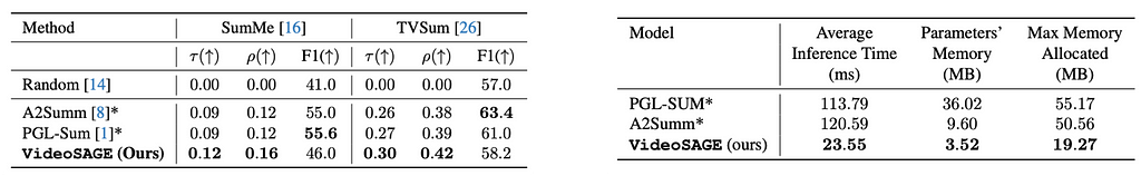
We show that this structured sparsity leads to comparable or improved results on video summarization datasets(SumMe and TVSum) show that VideoSAGE has comparable performance as existing state-of-the-art summarization approaches while consuming significantly lower memory and compute budgets. The tables below show the comparative results of our method, namely VideoSAGE, on performances and objective scores. This has recently been accepted in a workshop at CVPR 2024. The paper details and more results are available here.
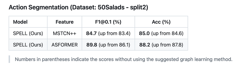
Similarly, we also pose the action segmentation problem as a node classification in such a sparse graph constructed from the input video. The GNN structure is similar to the above, except the last GNN layer is Graph Attention Network (GAT) instead of SageConv as used in the video summarization. We perform experiments of 50-Salads dataset. We leverage MSTCN or ASFormer as the stage 1 initial feature extractors. Next, we utilize our sparse, Bi-Directional GNN model that utilizes concurrent temporal “forward” and “backward” local message-passing operations. The GNN model further refine the final, fine-grain per-frame action prediction of our system. Refer to table 2 for the results.
In this section, we will describe how we can take the similar graph based approach where as nodes denote “objects” instead of one whole video frame. We will start with a specific example to describe the spatio-temporal graph approach.
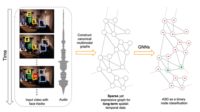
Figure 2 illustrates an overview of our framework designed for Active Speaker Detection (ASD) task. With the audio-visual data as input, we construct a multimodal graph and cast the ASD as a graph node classification task. Figure 3 demonstrates the graph construction process. First, we create a graph where the nodes correspond to each person within each frame, and the edges represent spatial or temporal relationships among them. The initial node features are constructed using simple and lightweight 2D convolutional neural networks (CNNs) instead of a complex 3D CNN or a transformer. Next, we perform binary node classification i.e. active or inactive speaker — on each node of this graph by learning a light-weight three-layer graph neural network (GNN). Graphs are constructed specifically for encoding the spatial and temporal dependencies among the different facial identities. Therefore, the GNN can leverage this graph structure and model the temporal continuity in speech as well as the long-term spatial-temporal context, while requiring low memory and computation.
You can ask why the graph construction is this way? Here comes the influence of the domain knowledge. The reason the nodes within a time distance that share the same face-id are connected with each other is to model the real-world scenario that if a person is taking at t=1 and the same person is talking at t=5, the chances are that person is talking at t=2,3,4. Why we connect different face-ids if they share the same time-stamp? That’s because, in general, if a person is talking others are most likely listening. If we had connected all nodes with each other and made the graph dense, the model not only would have required huge memory and compute, they would also have become noisy.
We perform extensive experiments on the AVA-ActiveSpeaker dataset. Our results show that SPELL outperforms all previous state-of-the-art (SOTA) approaches. Thanks to ~95% sparsity of the constructed graphs, SPELL requires significantly less hardware resources for the visual feature encoding (11.2M #Params) compared to ASDNet (48.6M #Params), one of the leading state-of-the-art methods of that time.
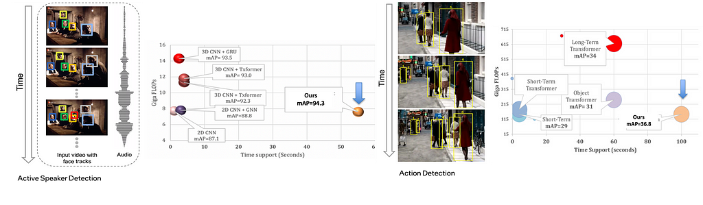
Refer to figure 3 below that shows the temporal context achieved by our methods on two different applications.
The hyper-parameter τ (= 0.9 second in our experiments) in SPELL imposes additional constraints on direct connectivity across temporally distant nodes. The face identities across consecutive timestamps are always connected. Below is the estimate of the effective temporal context size of SPELL. The AVA-ActiveSpeaker dataset contains 3.65 million frames and 5.3 million annotated faces, resulting in 1.45 faces per frame. Averaging 1.45 faces per frame, a graph with 500 to 2000 faces in sorted temporal order can span 345 to 1379 frames, corresponding to anywhere between 13 and 55 seconds for a 25 frame/second video. In other words, the nodes in the graph might have a time difference of about 1 minute, and SPELL is able to effectively reason over that long-term temporal window within a limited memory and compute budget. It is noteworthy that the temporal window size in MAAS is 1.9 seconds and TalkNet uses up to 4 seconds as long-term sequence-level temporal context.
The work on spatio-temporal graphs for active speaker detection has been published at ECCV 2022. The manuscript can be found here . In an earlier blog we provided more details.
The ASD problem setup in Ava active speaker dataset has access to the labeled faces and labeled face tracks as input to the problem setup. That largely simplifies the construction of the graph in terms of identifying the nodes and edges. For other problems, such as Action Detection, where the ground truth object (person) locations and tracks are not provided, we use pre-processing to detect objects and object tracks, then utilize SPELL for the node classification problem. Similar to the previous case, we utilize domain knowledge and contruct a sparse graph. The “object-centric” graphs are first created keeping the underlying application in mind.
On average, we achieve ~90% sparse graphs; a key difference compared to visual transformer-based methods which rely on dense General Matrix Multiply (GEMM) operations. Our sparse GNNs allow us to (1) achieve slightly better performance than transformer-based models; (2) aggregate temporal context over 10x longer windows compared to transformer-based models (100s vs 10s); and (3) Achieve 2–5X compute savings compared to transformers-based methods.
We have open-sourced our software library, GraVi-T. At present, GraVi-T supports multiple video understanding applications, including Active Speaker Detection, Action Detection, Temporal Segmentation, Video Summarization. See our opensource software library GraVi-T to more on the applications.
Compared to transformers, our graph approach can aggregate context over 10x longer video, consumes ~10x lower memory and 5x lower FLOPs. Our first and major work in this topic (Active Speaker Detection) was published at ECCV’22. Watch out for our latest publication at upcoming CVPR 2024 on video summarization aka video highlights reels creation.
Our approach of modeling video as a sparse graph outperformed complex SOTA methods on several applications. It secured top places in multiple leaderboards. The list includes ActivityNet 2022, Ego4D audio-video diarization challenge at ECCV 2022, CVPR 2023. Source code for the training the past challenge winning models are also included in our open-sourced software library, GraVi-T.
We are excited about this generic, lightweight and efficient framework and are working towards other new applications. More exciting news coming soon !!!
Long-form video representation learning (Part 1: Video as graphs) was originally published in Towards Data Science on Medium, where people are continuing the conversation by highlighting and responding to this story.
Originally appeared here:
Long-form video representation learning (Part 1: Video as graphs)
Go Here to Read this Fast! Long-form video representation learning (Part 1: Video as graphs)
Feeling inspired to write your first TDS post? We’re always open to contributions from new authors.
New LLMs continue to arrive on the scene almost daily, and the tools and workflows they make possible proliferate even more quickly. We figured it was a good moment to take stock of some recent conversations on this ever-shifting terrain, and couldn’t think of a better way to do that than by highlighting some of our strongest articles from the past couple of weeks.
The lineup of posts we put together tackle high-level questions and nitty-gritty problems, so whether you’re interested in AI ethics, the evolution of open-source technology, or innovative RAG approaches, we’re certain you’ll find something here to pique your interest. Let’s dive in.

As they always do, our authors branched out to many other topics in recent weeks, producing some top-notch articles; here’s a representative sample:
Thank you for supporting the work of our authors! We love publishing articles from new authors, so if you’ve recently written an interesting project walkthrough, tutorial, or theoretical reflection on any of our core topics, don’t hesitate to share it with us.
Until the next Variable,
TDS Team
Open-Source Models, Temperature Scaling, Re-Ranking, and More: Don’t Miss Our Latest LLM Must-Reads was originally published in Towards Data Science on Medium, where people are continuing the conversation by highlighting and responding to this story.
Originally appeared here:
Open-Source Models, Temperature Scaling, Re-Ranking, and More: Don’t Miss Our Latest LLM Must-Reads
“When life gives you chickens, let AI handle the fowl play.” — Unknown Engineer.
Why on earth do we need simulations? What is the advantage we can get by sampling something and getting an average? But that is never only this. Real life is usually far more complex compared to simplistic tasks we encounter in computer science classes. Sometimes we can’t find an analytical solution, we can’t find population parameters. Sometimes we have to build a model to reflect specifics of the system’s dynamics, we have to run simulations to study the underlying processes so as to gain a better understanding of real-world situations. Simulation modelling provides an invaluable tool for systems design and engineering across a range of industries and applications. It helps to analyse system performance, identify potential bottlenecks and inefficiencies, thus allowing for iterative refinements and improvements.
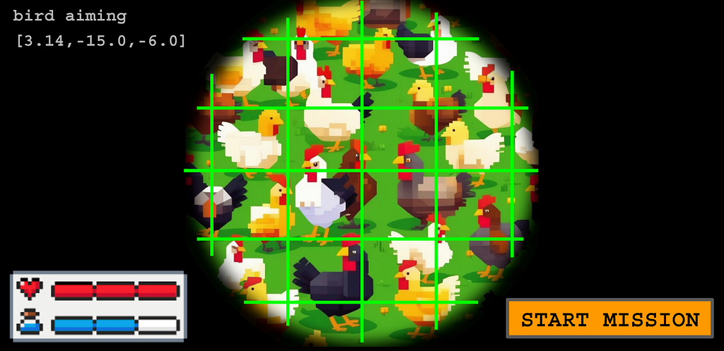
Speaking about our very special challenge, here, we are going to create an FSM simulation replicating the behavior of an AI-assisted security system for lawn monitoring and cleaning. In particular, we will tackle the task of simulating processes to intelligently manage the coming and going of birds through object detection and water sprinkling subsystems. In the previous article, you had been introduced to the theory and design principles on finite state machines (FSM) for dealing with the infamous Chicken-and-Turkey (CaT) problem, resulting in the creation of a model that describes complex lawn scenarios at a high level of abstraction. Through this article, we will further investigate the topic of practical aspects of an FSM-based simulation for leveraging the real-life system operation. In addition, we are going to implement the FSM simulation in Python so that we can later improve it via optimization and XAI techniques. By the end of the tutorial, you’ll have a fully functional FSM solution along with a better understanding of simulation modelling for solving engineering problems.
Disclaimer: This work is a part of the “Bird by Bird using Deep Learning” series and is devoted to modelling and simulation of real-life systems for computer vision applications using finite automata. All actors, states, events and outputs are the products of the FSM design process for educational purposes only. Any resemblance to actual persons, birds, or real events is purely coincidental.
“When asked about systems design sans abstractions, just describe if-then loops for real-life scenarios, making sure to stutter while juggling multiple conditions. Then, gracefully retreat, leaving these trivialities behind.” — Unknown Engineer.
Simulation, a special case of mathematical modelling, involves creating simplified representations of real-world systems to understand their behavior under various conditions. At its core, a model is to capture intrinsic patterns of a real-life system through equations, while simulation relates to the algorithmic approximation of these equations by running a program. This process enables generation of simulation results, facilitating comparison with theoretical assumptions and driving improvements in the actual system. Simulation modelling allows to provide insights on the system behavior and predict outcomes when it’s too expensive and/or challenging to run real experiments. It can be especially useful when an analytical solution is not feasible (e.g., warehouse management processes).
When dealing with the CaT-problem, the objective is clear: we want to maintain a pristine lawn and save resources. Rather than relying on traditional experimentation, we opt for a simulation-based approach to find a setup that allows us to minimize water usage and bills. To achieve this, we will develop an FSM-based model that reflects the key system processes, including bird intrusion, bird detection, and water sprinkling. Throughout the simulation, we will then assess the system performance to guide further optimization efforts towards improved efficiency on bird detection.
Using if-else conditional branching for system modelling is a naïve solution that will ultimately lead to increased complexity and error-proneness by design, making further development and maintenance more difficult. Below you find how to (not) describe a simple chicken-on-the-lawn system, considering an example of the simple FSM we discussed earlier (see Figure 1 for FSM state transition diagram with simplified CaT- system scenarios).
# import functions with input events and actions
from events import (
   simulate_chicken_intrusion,
   initiate_shooing_chicken,
)
from actions import (
  spoil_the_lawn,
  start_lawn_cleaning,
  one_more_juice
)

# define states
START = 0
CHICKEN_PRESENT = 1
NO_CHICKEN = 2
LAWN_SPOILING = 3
ENGINER_REST = 4
END = 5

# initialise simulation step and duration
sim_step = 0
max_sim_steps = 8

# initialise states
prev_state = None
current_state = START

# monitor for events
while current_state != END:
   # update state transitions
   if current_state == START:
       current_state = NO_CHICKEN
       prev_state = START
   elif current_state == NO_CHICKEN:
       if prev_state == CHICKEN_PRESENT:
           start_lawn_cleaning()
       if simulate_chicken_intrusion():
           current_state = CHICKEN_PRESENT
       else:
           current_state = ENGINER_REST
       prev_state = NO_CHICKEN
   elif current_state == CHICKEN_PRESENT:
       if initiate_shooing_chicken():
           current_state = NO_CHICKEN
       else:
           current_state = LAWN_SPOILING
       prev_state = CHICKEN_PRESENT
   elif current_state == LAWN_SPOILING:
       spoil_the_lawn()
       current_state = CHICKEN_PRESENT
       prev_state = LAWN_SPOILING
   elif current_state == ENGINER_REST:
       one_more_juice()
       current_state = NO_CHICKEN
       prev_state = ENGINER_REST

   sim_step += 1
   if sim_step >= max_sim_steps:
       current_state = END
In this code snippet, we define constants to represent each state of the FSM (e.g., CHICKEN_PRESENT). Then, we initialize the current state to START and continuously monitor for events within a while loop, simulating the behavior of the simplified system. Based on the current state and associated events, we use if-else conditional branching instructions to switch between states and invoke corresponding actions. A state transition can have side effects, such as initiating the process of the lawn spoiling for chickens and starting the lawn cleaning for the engineer. Here, functionality related to input events and actions indicates processes that can be automated, so we mock importing the associated functions for simplicity. Note, that whilst chickens can spoil a lawn nearly endlessly, excessive quantities of juice are fraught with the risk of hyperhydration. Be careful with this and don’t forget to add constraints on the duration of your simulation. In our case, this will be the end of the day, as defined by the `max_sim_steps` variable. Looks ugly, right?
This should work, but imagine how much time it would take to update if-else instructions if we wanted to extend the logic, repeating the same branching and switching between states over and over. As you can imagine, as the number of states and events increases, the size of the system state space grows rapidly. Unlike if-else branching, FSMs are really good at handling complex tasks, allowing complex systems to be decomposed into manageable states and transitions, hence enhancing code modularity and scalability. Here, we are about to embark on a journey in implementing the system behavior using finite automata to reduce water usage for AI-system operation without compromising accuracy on bird detection.
“Ok, kiddo, we are about to create a chicken now.” — Unknown Engineer.
In this section, we delve into the design choices underlying FSM implementation, elucidating strategies to streamline the simulation process and maximize its utility in real-world system optimization. To build the simulation, we first need to create a model representing the system based on our assumptions about the underlying processes. One way to do this is to start with encapsulating functionally for individual states and transitions. Then we can combine them to create a sequence of events by replicating a real system behavior. We also want to track output statistics for each simulation run to provide an idea of its performance. What we want to do is watch how the system evolves over time given variation in conditions (e.g., stochastic processes of birds spawning and spoiling the lawn given a probability). For this, let’s start with defining and arranging building blocks we are going to implement later on. Here is the plan:
The source code used for this tutorial can be found in this GitHub repository: https://github.com/slipnitskaya/Bird-by-Bird-AI-Tutorials.
First, we need to create a class hierarchy for our simulation, spanning from base classes for states to a more domain specific yard simulation subclass. We will use `@abc.abstractmethod` and `@property` decorators to mark abstract methods and properties, respectively. In the AbstractSimulation class, we will define `step()` and `run()` abstract methods to make sure that child classes implement them.
class AbstractSimulation(abc.ABC):
   @abc.abstractmethod
   def step(self) -> Tuple[int, List['AbstractState']]:
       pass

   @abc.abstractmethod
   def run(self) -> Iterator[Tuple[int, List['AbstractState']]]:
       pass
Similar applies to AbstractState, which defines an abstract method `transit()` to be implemented by subclasses:
class AbstractState(abc.ABC):
   def __init__(self, state_machine: AbstractSimulation):
       super().__init__()
       self.state_machine = state_machine

   def __eq__(self, other):
       return self.__class__ is other.__class__

   @abc.abstractmethod
   def transit(self) -> 'AbstractState':
       pass
For our FSM, more specific aspects of the system simulation will be encapsulated in the AbstractYardSimulation class, which inherits from AbstractSimulation. As you can see in its name, AbstractYardSimulation outlines the domain of simulation more precisely, so we can define some extra methods and properties that are specific to the yard simulation in the context of the CaT problem, including `simulate_intrusion()`, `simulate_detection()`, `simulate_sprinkling()`, `simulate_spoiling()`.
We will also create an intermediate abstract class named AbstractYardState to enforce typing consistency in the hierarchy of classes:
class AbstractYardState(AbstractState, abc.ABC):
   state_machine: AbstractYardSimulation
Now, let’s take a look at the inheritance tree reflecting an entity named Target and its descendants.
Target behavior is a cornerstone of our simulation, as it affects all the aspects towards building an effective model along with its optimization downstream. Figure 1 shows a class diagram for the target classes we are going to implement.
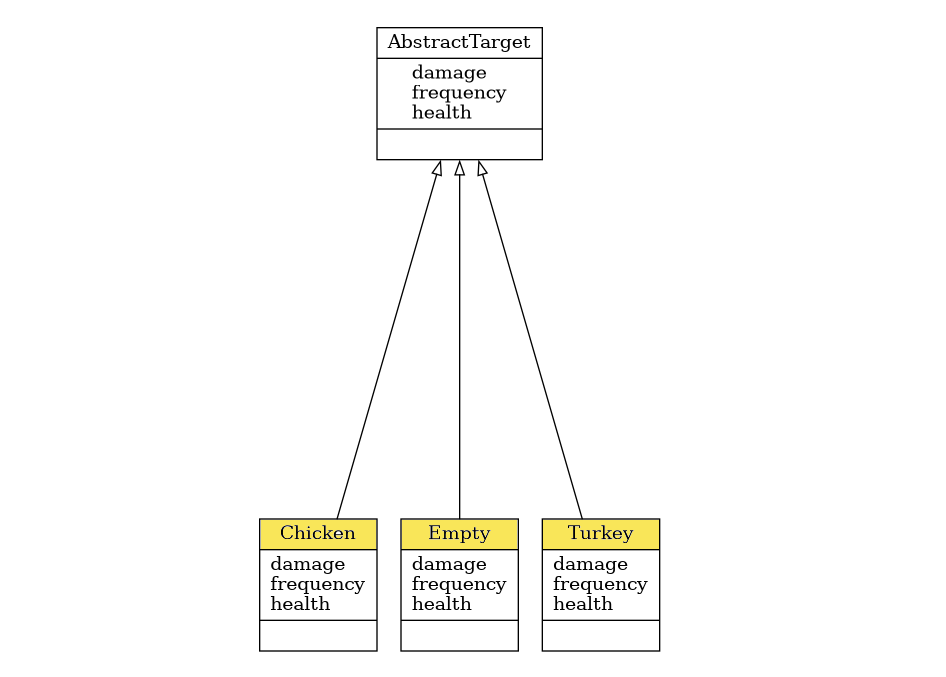
For our system, it’s important to note that a target appears with a certain frequency, it may cause some damage to the lawn, and it also has a health property. The latter is related to the size of the target, which may differ, thus a water gun can aim for either smaller or larger targets (which, in turn, affects the water consumption). Consequently, a large target has a lot of health points, so a small water stream will not be able to effectively manage it.
To model targets trespassing the lawn with different frequencies we also create the associated property. Here we go:
class AbstractTarget(int, abc.ABC):
   @property
   @abc.abstractmethod
   def health(self) -> float:
       pass

   @property
   @abc.abstractmethod
   def damage(self) -> float:
       pass

   @property
   @abc.abstractmethod
   def frequency(self) -> float:
       pass
Note that in our implementation we want the target objects to be valid integers, which will be of use for modelling randomness in the simulation.
Next, we create child classes to implement different kinds of targets. Below is the code of the class Chicken, where we override abstract methods inherited from the parent:
class Chicken(AbstractTarget):
   @property
   def health(self) -> float:
       return 4

   @property
   def damage(self) -> float:
       return 10

   @property
   def frequency(self) -> float:
       return 9
We repeat the similar procedure for remaining Turkey and Empty classes. In the case of Turkey, health and damage parameters will be set to 7 and 17, respectively (let’s see how we can handle these bulky ones with our AI-assisted system). Empty is a special type of Target that refers to the absence of either bird species on the lawn. Although we can’t assign to its health and damage properties other values than 0, an unconditional (i.e. not caused by the engineer) birdlessness on the lawn has a non-zero probability reflected by the frequency value of 9.
Now imagine a bird in its natural habitat. It can exhibit a wide variety of agonistic behaviors and displays. In the face of challenge, animals may employ a set of adaptive strategies depending on the circumstances, including fight, or flight responses and other intermediate actions. Following up on the previous article on the FSM design and modelling, you may remember that we already described the key components of the CaT system, which we will use for the actual implementation (see Table 2 for FSM inputs describing the events triggering state changes).
In the realm of the FSM simulation, a bird can be viewed as an independent actor triggering a set of events: trespassing the yard, spoiling the grass, and so on. In particular, we expect the following sequential patterns in case of an optimistic scenario (success in bird detection and identification, defense actions): a bird invades the yard before possibly being recognized by the CV-based bird detector in order to move ahead with water sprinkling module, those configuration is dependent on the invader class predicted upstream. This way, the bird can be chased away successfully (hit) or not (miss). For this scenario (success in bird detection, class prediction, defense actions), the bird, eventually, escapes from the lawn. Mission complete. Tadaa!
You may remember that the FSM can be represented graphically as a state transition diagram, which we covered in the previous tutorial (see Table 3 for FSM state transition table with next-stage transition logic). Considering that, now we will create subclasses of AbstractYardState and override the `transit()` method to specify transitions between states based on the current state and events.
Start is the initial state from which the state machine transits to Spawn.
class Start(AbstractYardState):
   def transit(self) -> 'Spawn':
       return Spawn(self.state_machine)
From Spawn, the system can transit to one of the following states: Intrusion, Empty, or End.
class Spawn(AbstractYardState):
   def transit(self) -> Union['Intrusion', 'Empty', 'End']:
       self.state_machine.stayed_steps += 1

       self.state_machine.simulate_intrusion()

       next_state: Union['Intrusion', 'Empty', 'End']
       if self.state_machine.max_steps_reached:
           next_state = End(self.state_machine)
       elif self.state_machine.bird_present:
           next_state = Intrusion(self.state_machine)
       else:
           next_state = Empty(self.state_machine)

       return next_state
Transition to the End state happens if we reach the limit on the number of simulation time steps. The state machine switches to Intrusion if a bird invades or is already present on the lawn, while Empty is the next state otherwise.
Both Intrusion and Empty states are followed by a detection attempt, so they share a transition logic. Thus, we can reduce code duplication by creating a parent class, namely IntrusionStatus, to encapsulate this logic, while aiming the subclasses at making the actual states of the simulation Intrusion and Empty distinguishable at the type level.
class IntrusionStatus(AbstractYardState):
   intruder_class: Target

   def transit(self) -> Union['Detected', 'NotDetected']:
       self.state_machine.simulate_detection()
       self.intruder_class = self.state_machine.intruder_class

       next_state: Union['Detected', 'NotDetected']
       if self.state_machine.predicted_bird:
           next_state = Detected(self.state_machine)
       else:
           next_state = NotDetected(self.state_machine)

       return next_state
We apply a similar approach to the Detected and NotDetected classes, those superclass DetectionStatus handles target prediction.
class DetectionStatus(AbstractYardState):
   detected_class: Target

   def transit(self) -> 'DetectionStatus':
       self.detected_class = self.state_machine.detected_class

       return self
However, in contrast to the Intrusion/Empty pair, the NotDetected class introduces an extra transition logic steering the simulation flow with respect to the lawn contamination/spoiling.
class Detected(DetectionStatus):
   def transit(self) -> 'Sprinkling':
       super().transit()

       return Sprinkling(self.state_machine)


class NotDetected(DetectionStatus):
   def transit(self) -> Union['Attacking', 'NotAttacked']:
       super().transit()

       next_state: Union['Attacking', 'NotAttacked']
       if self.state_machine.bird_present:
           next_state = Attacking(self.state_machine)
       else:
           next_state = NotAttacked(self.state_machine)

       return next_state
The Detected class performs an unconditional transition to Sprinkling. For its antagonist, there are two possible next states, depending on whether a bird is actually on the lawn. If the bird is not there, no poops are anticipated for obvious reasons, while there may potentially be some grass cleaning needed otherwise (or not, the CaT universe is full of randomness).
Getting back to Sprinkling, it has two possible outcomes (Hit or Miss), depending on whether the system was successful in chasing the bird away (this time, at least).
class Sprinkling(AbstractYardState):
   def transit(self) -> Union['Hit', 'Miss']:
       self.state_machine.simulate_sprinkling()

       next_state: Union['Hit', 'Miss']
       if self.state_machine.hit_successfully:
           next_state = Hit(self.state_machine)
       else:
           next_state = Miss(self.state_machine)

       return next_state
Note: The Hit state does not bring a dedicated transition logic and is included to follow semantics of the domain of wing-aided shitting on the grass. Omitting it will cause the Shooting state transition to Leaving directly.
class Hit(AbstractYardState):
   def transit(self) -> 'Leaving':
       return Leaving(self.state_machine)
If the water sprinkler was activated and there was no bird on the lawn (detector mis-predicted the bird), the state machine will return to Spawn. In case the bird was actually present and we missed it, there’s a possibility of bird spoils on the grass.
class Miss(AbstractYardState):
   def transit(self) -> Union['Attacking', 'Spawn']:
       next_state: Union['Attacking', 'Spawn']
       if self.state_machine.bird_present:
           next_state = Attacking(self.state_machine)
       else:
           next_state = Spawn(self.state_machine)

       return next_state
Eventually, the attacking attempt can result in a real damage to the grass, as reflected by the Attacking class and its descendants:
class Attacking(AbstractYardState):
   def transit(self) -> Union['Attacked', 'NotAttacked']:
       self.state_machine.simulate_spoiling()

       next_state: Union['Attacked', 'NotAttacked']
       if self.state_machine.spoiled:
           next_state = Attacked(self.state_machine)
       else:
           next_state = NotAttacked(self.state_machine)

       return next_state


class Attacked(AfterAttacking):
   def transit(self) -> Union['Leaving', 'Spawn']:
       return super().transit()


class NotAttacked(AfterAttacking):
   def transit(self) -> Union['Leaving', 'Spawn']:
       return super().transit()
We can employ the same idea as for the Intrusion status and encapsulate the shared transition logic into a superclass AfterAttacking, resulting in either Leaving or returning to the Spawn state:
class AfterAttacking(AbstractYardState):
   def transit(self) -> Union['Leaving', 'Spawn']:
       next_state: Union['Leaving', 'Spawn']
       if self.state_machine.max_stay_reached:
           next_state = Leaving(self.state_machine)
       else:
           next_state = Spawn(self.state_machine)

       return next_state
What happens next? When the simulation reaches the limit of steps, it stucks in the End state:
class End(AbstractYardState):
   def transit(self) -> 'End':
       return self
In practice, we don’t want the program to execute endlessly. So, subsequently, once the simulation detects a transition into the End state, it shuts down.
“In the subtle world of bird detection, remember: while a model says “no chickens detected,” a sneaky bird may well be on the lawn unnoticed. This discrepancy stands as a call to refine and enhance our AI systems.” — Unknown Engineer.
Now, we’d like to simulate a process of birds trespassing the lawn, spoiling it and leaving. To do so, we will turn to a kind of simulation modelling called discrete-event simulation. We will reproduce the system behavior by analyzing the most significant relationships between its elements and developing a simulation based on finite automata mechanics. For this, we have to consider the following aspects:
Now, it’s time to explore the magic of probability to simulate these processes using the implemented FSM. For that, we need to create a YardSimulation class that encapsulates the simulation logic. As said, the simulation is more than an FSM. The same applies to the correspondences between simulation steps and state machine transitions. That is, the system needs to perform several state transitions to switch to the next time step.
Here, the `step()` method handles transitions from the current to the next state and invokes the FSM’s method `transit()` until the state machine returns into the Spawn state or reaches End.
def step(self) -> Tuple[int, List[AbstractYardState]]:
   self.step_idx += 1

   transitions = list()
   while True:
       next_state = self.current_state.transit()
       transitions.append(next_state)
       self.current_state = next_state

       if self.current_state in (Spawn(self), End(self)):
           break

   return self.step_idx, transitions
In the `run()` method, we call `step()` in the loop and yield its outputs until the system transits to the End step:
def run(self) -> Iterator[Tuple[int, List[AbstractYardState]]]:
   while self.current_state != End(self):
       yield self.step()
The `reset()` method resets the FSM memory after the bird leaves.
def reset(self) -> 'YardSimulation':
   self.current_state = Start(self)
   self.intruder_class = Target.EMPTY
   self.detected_class = Target.EMPTY
   self.hit_successfully = False
   self.spoiled = False
   self.stayed_steps = 0

   return self
A bird is leaving when either it’s successfully hit by the water sprinkler or it stays too long on the lawn (e.g., assuming it got bored). The latter is equivalent to having a bird present on the lawn during 5 simulation steps (= minutes). Not that long, who knows, maybe the neighbor’s lawn looks more attractive.
Next, let’s implement some essential pieces of our system’s behavior. For (1), if no bird is present on the lawn (true intruder class), we try to spawn the one.
def simulate_intrusion(self) -> Target:
   if not self.bird_present:
       self.intruder_class = self.spawn_target()

   return self.intruder_class
Here, spawning relates to the live creation of the trespassing entity (bird or nothing).
@property
def bird_present(self) -> bool:
   return self.intruder_class != Target.EMPTY
Then (2), the CV-based system — that is described by a class confusion matrix — tries to detect and classify the intruding object. For this process, we simulate a prediction generation, while keeping in mind the actual intruder class (ground truth).
def simulate_detection(self) -> Target:
   self.detected_class = self.get_random_target(self.intruder_class)

   return self.detected_class
Detector works on every timestep of the simulation, as the simulated system doesn’t know the ground truth (otherwise, why would we need the detector?). If the detector identifies a bird (point 3), we try to chase it away with the water sprinkler tuned to a specific water flow rate that depends on the detected target class:
def simulate_sprinkling(self) -> bool:
   self.hit_successfully = self.bird_present and (self.rng.uniform() <= self.hit_proba) and self.target_vulnerable

   return self.hit_successfully
Regardless of the success of the sprinkling, the system consumes water anyway. Hit success criteria includes the following conditions: a bird was present on the lawn (a), water sprinkler hit the bird (b), the shot was adequate/sufficient to treat the bird of a given size ©. Note, that © the chicken “shot” won’t treat the turkey, but applies otherwise.
Spoiling part (4) — a bird can potentially mess up with the grass. If this happens, the lawn damage rate increases (obviously).
def simulate_spoiling(self) -> bool:
   self.spoiled = self.bird_present and (self.rng.uniform() <= self.shit_proba)
   if self.spoiled:
       self.lawn_damage[self.intruder_class] += self.intruder_class.damage

   return self.spoiled
Now we have all the essentials to simulate a single time step for the CaT problem we are going to handle. Simulation time!
Now, we are all set to employ our FSM simulation to emulate an AI-assisted lawn security system across different settings. While running a yard simulation, the `YardSimulation.run()` method iterates over a sequence of state transitions until the system reaches the limit of steps. For this, we instantiate a simulation object (a.k.a. state machine), setting the `num_steps` argument that reflects the total amount of the simulation timesteps (let’s say 12 hours or daytime) and `detector_matrix` that relates to the confusion matrix of the CV-based bird detector subsystem trained to predict chickens and turkeys:
sim = YardSimulation(detector_matrix=detector_matrix, num_steps=num_steps)
Now we can run the FSM simulation and print state transitions that the FSM undergoes at every timestep:
for step_idx, states in sim.run():
   print(f't{step_idx:0>3}: {" -> ".join(map(str, states))}')
In addition, we accumulate simulation statistics related to the water usage for bird sprinkling (`simulate_sprinkling`) and grass cleaning after birds arrive (`simulate_spoiling`).
def simulate_sprinkling(self) -> bool:
   ...
   self.water_consumption[self.detected_class] += self.detected_class.health
   ...


def simulate_spoiling(self) -> bool:
   ...
   if self.spoiled:
       self.lawn_damage[self.intruder_class] += self.intruder_class.damage
   ...
When the simulation reaches its limit, we can then compute the total water consumption by the end of the day for each of the categories. What we would like to see is what happens after each run of the simulation.
water_sprinkling_total = sum(sim.water_consumption.values())
lawn_damage_total = sum(sim.lawn_damage.values())
Finally, let’s conduct experiments to assess how the system can perform given changes in the computer vision-based subsystem. To that end, we will run simulations using YardSimulation.run()` method for 100 trials for a non-trained (baseline) and perfect detection matrices:
detector_matrix_baseline = np.full(
     (len(Target),) * 2,  # size of the confusion matrix (3 x 3)
     len(Target) ** -1    # prediction probability for each class is the same and equals to 1/3
)
detector_matrix_perfect = np.eye(len(Target))
Thereafter, we can aggregate and compare output statistics related to the total water usage for target sprinkling and lawn cleaning for different experimental settings:
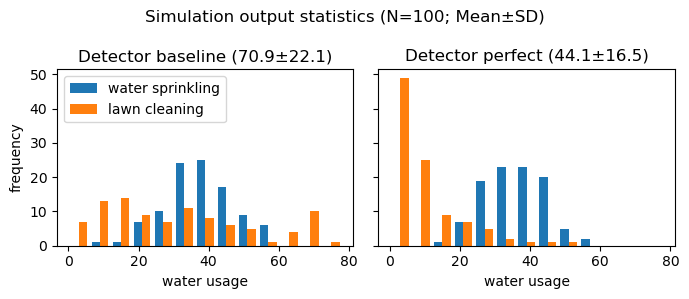
A comparison of summary results across experiments reveals that having a better CV model would contribute to increased efficiency in minimizing water usage by 37.8% (70.9 vs. 44.1), compared to the non-trained baseline detector for birds under the given input parameters and simulation conditions — a concept both intuitive and anticipated. But what does “better” mean quantitatively? Is it worth fiddling around with refining the model? The numerical outcomes demonstrate the value of improving the model, motivating further refinement efforts. Going forward, we will use the resulting statistics as an objective for global optimization to improve efficiency of the bird detection subsystem and cut down on water consumption for system operation and maintenance, making the engineer a little happier.
To sum up, simulation modelling is a useful tool that can be used to estimate efficiency of processes, enable rapid testing of anticipated changes, and understand how to improve processes through operation and maintenance. Through this article, you have gained a better understanding on practical applications of simulation modelling for solving engineering problems. In particular, we’ve covered the following:
Focusing on improving resource efficiency, in the follow-up articles, you will discover how to address a non-analytic optimization problem of the water cost reduction by applying Monte-Carlo and eXplainable AI (XAI) methods to enhance the computer vision-based bird detection subsystem, thus advancing our simulated AI-assisted lawn security system.
What are other important concepts in simulation modelling and optimization for vision projects? Find out more on Bird by Bird Tech.
Bird by Bird using Finite Automata was originally published in Towards Data Science on Medium, where people are continuing the conversation by highlighting and responding to this story.
Originally appeared here:
Bird by Bird using Finite Automata
Go Here to Read this Fast! Bird by Bird using Finite Automata


We code examples using Altair, Bokeh, Plotly, Pandas Plot and Matplotlib, to illustrate the pros and cons of each one
Originally appeared here:
Streamlit Supports 5 Important Data Visualization Libraries — Which to Choose?