Tag: AI

  • How to Evaluate Your Predictions

    Jeffrey Näf

    Be mindful of the measure you choose

    Photo by Isaac Smith on Unsplash

    Testing and benchmarking machine learning models by comparing their predictions on a test set, even after deployment, is of fundamental importance. To do this, one needs to think of a measure or score that takes a prediction and a test point and assigns a value measuring how successful the prediction is with respect to the test point. However, one should think carefully about which scoring measure is appropriate. In particular, when choosing a method to evaluate a prediction we should adhere to the idea of proper scoring rules. I only give a loose definition of this idea here, but basically, we want a score that is minimized at the thing we want to measure!

    As a general rule: One can use MSE to evaluate mean predictions, MAE to evaluate median predictions, the quantile score to evaluate more general quantile predictions and the energy or MMD score to evaluate distributional predictions.

    Consider a variable you want to predict, say a random variable Y, from a vector of covariates X. In the example below, Y will be income and X will be certain characteristics, such as age and education. We learned a predictor f on some training data and now we predict Y as f(x). Usually, when we want to predict a variable Y as well as possible we predict the expectation of y given x, i.e. f(x) should approximate E[Y | X=x]. But more generally, f(x) could be an estimator of the median, other quantiles, or even the full conditional distribution P(Y | X=x).

    Now for a new test point y, we want to score your prediction, that is you want a function S(y,f(x)), that is minimized (in expectation) when f(x) is the best thing you can do. For instance, if we want to predict E[Y | X=x], this score is given as the MSE: S(y, f(x))= (y-f(x))².

    Here we study the principle of scoring the predictor f over at test set of (y_i,x_i), i=1,…,ntest in more detail. In all examples we will compare the ideal estimation method to an other that is clearly wrong, or naive, and show that our scores do what they are supposed to.

    The Example

    To illustrate things, I will simulate a simple dataset that should mimic income data. We will use this simple example throughout this article to illustrate the concepts.

    library(dplyr)


    #Create some variables:
    # Simulate data for 100 individuals
    n <- 5000

    # Generate age between 20 and 60
    age <- round(runif(n, min = 20, max = 60))

    # Define education levels
    education_levels <- c("High School", "Bachelor's", "Master's")

    # Simulate education level probabilities
    education_probs <- c(0.4, 0.4, 0.2)

    # Sample education level based on probabilities
    education <- sample(education_levels, n, replace = TRUE, prob = education_probs)

    # Simulate experience correlated with age with some random error
    experience <- age - 20 + round(rnorm(n, mean = 0, sd = 3))

    # Define a non-linear function for wage
    wage <- exp((age * 0.1) + (case_when(education == "High School" ~ 1,
    education == "Bachelor's" ~ 1.5,
    TRUE ~ 2)) + (experience * 0.05) + rnorm(n, mean = 0, sd = 0.5))

    hist(wage)

    Although this simulation may be oversimplified, it reflects certain well-known characteristics of such data: older age, advanced education, and greater experience are all linked to higher wages. The use of the “exp” operator results in a highly skewed wage distribution, which is a consistent observation in such datasets.

    Wage distribution over the whole simulated population. Source: Author

    Crucially, this skewness is also present when we fix age, education and experience to certain values. Let’s imagine we look at a specific person, Dave, who is 30 years old, has a Bachelor’s in Economics and 10 years of experience and let’s look at his actual income distribution according to our data generating process:

    ageDave<-30
    educationDave<-"Bachelor's"
    experienceDave <- 10


    wageDave <- exp((ageDave * 0.1) + (case_when(educationDave == "High School" ~ 1,
    educationDave == "Bachelor's" ~ 1.5,
    TRUE ~ 2)) + (experienceDave * 0.05) + rnorm(n, mean = 0, sd = 0.5))

    hist(wageDave, main="Wage Distribution for Dave", xlab="Wage")
    Wage distrbution for Dave. Source: Author

    Thus the distribution of possible wages of Dave, given the information we have about him, is still highly skewed.

    We also generate a test set of several people:


    ## Generate test set
    ntest<-1000

    # Generate age between 20 and 60
    agetest <- round(runif(ntest, min = 20, max = 60))


    # Sample education level based on probabilities
    educationtest <- sample(education_levels, ntest, replace = TRUE, prob = education_probs)

    # Simulate experience correlated with age with some random error
    experiencetest <- agetest - 20 + round(rnorm(ntest, mean = 0, sd = 3))


    ## Generate ytest that we try to predict:

    wagetest <- exp((agetest * 0.1) + (case_when(educationtest == "High School" ~ 1,
    educationtest == "Bachelor's" ~ 1.5,
    TRUE ~ 2)) + (experiencetest * 0.05) + rnorm(ntest, mean = 0, sd = 0.5))

    We now start simple and first look at the scores for mean and median prediction.

    The scores for mean and median prediction

    In data science and machine learning, interest often centers on a single number that signifies the “center” or “middle” of the distribution we aim to predict, namely the (conditional) mean or median. To do this we have the mean squared error (MSE):

    and the mean absolute error (MAE):

    An important takeaway is that the MSE is the appropriate metric for predicting the conditional mean, while the MAE is the measure to use for the conditional median. Mean and median are not the same thing for skewed distributions like the one we study here.

    Let us illustrate this for the above example with very simple estimators (that we would not have access to in real life), just for illustration:

    conditionalmeanest <-
    function(age, education, experience, N = 1000) {
    mean(exp((age * 0.1) + (
    case_when(
    education == "High School" ~ 1,
    education == "Bachelor's" ~ 1.5,
    TRUE ~ 2
    )
    ) + (experience * 0.05) + rnorm(N, mean = 0, sd = 0.5)
    ))
    }


    conditionalmedianest <-
    function(age, education, experience, N = 1000) {
    median(exp((age * 0.1) + (
    case_when(
    education == "High School" ~ 1,
    education == "Bachelor's" ~ 1.5,
    TRUE ~ 2
    )
    ) + (experience * 0.05) + rnorm(N, mean = 0, sd = 0.5)
    ))
    }

    That is we estimate mean and median, by simply simulating from the model for fixed values of age, education, and experience (this would be a simulation from the correct conditional distribution) and then we simply take the mean/median of that. Let’s test this on Dave:


    hist(wageDave, main="Wage Distribution for Dave", xlab="Wage")
    abline(v=conditionalmeanest(ageDave, educationDave, experienceDave), col="darkred", cex=1.2)
    abline(v=conditionalmedianest(ageDave, educationDave, experienceDave), col="darkblue", cex=1.2)

    Blue: estimated conditional median of Dave, Red: estimated conditional mean of Dave. Source: Author

    Clearly the mean and median are different, as one would expect from such a distribution. In fact, as is typical for income distributions, the mean is higher (more influenced by high values) than the median.

    Now let’s use these estimators on the test set:

    Xtest<-data.frame(age=agetest, education=educationtest, experience=experiencetest)

    meanest<-sapply(1:nrow(Xtest), function(j) conditionalmeanest(Xtest$age[j], Xtest$education[j], Xtest$experience[j]) )
    median<-sapply(1:nrow(Xtest), function(j) conditionalmedianest(Xtest$age[j], Xtest$education[j], Xtest$experience[j]) )

    This gives a diverse range of conditional mean/median values. Now we calculate MSE and MAE:

    (MSE1<-mean((meanest-wagetest)^2))
    (MSE2<-mean((median-wagetest)^2))

    MSE1 < MSE2
    ### Method 1 (the true mean estimator) is better than method 2!

    # but the MAE is actually worse of method 1!
    (MAE1<-mean(abs(meanest-wagetest)) )
    (MAE2<-mean( abs(median-wagetest)))

    MAE1 < MAE2
    ### Method 2 (the true median estimator) is better than method 1!

    This shows what is known theoretically: MSE is minimized for the (conditional) expectation E[Y | X=x], while MAE is minimized at the conditional median. In general, it does not make sense to use the MAE when you try to evaluate your mean prediction. In a lot of applied research and data science, people use the MAE or both to evaluate mean predictions (I know because I did it myself). While this may be warranted in certain applications, this can have serious consequences for distributions that are not symmetric, as we saw in this example: When looking at the MAE, method 1 looks worse than method 2, even though the former estimates the mean correctly. In fact, in this highly skewed example, method 1 should have a lower MAE than method 2.

    To score conditional mean prediction use the mean squared error (MSE) and not the mean absolute error (MAE). The MAE is minimized for the conditional median.

    Scores for quantile and interval prediction

    Assume we want to score an estimate f(x) of the quantile q_x such that

    Simple quantile illustration. Source: Author

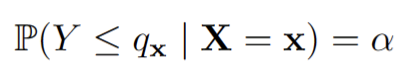
    In this case, we can consider the quantile score:

    whereby

    To unpack this formula, we can consider two cases:

    (1) y is smaller than f(x):

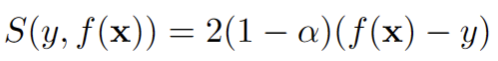
    i.e. we incur a penalty which gets bigger the further away y is from f(x).

    (2) y is larger than f(x):

    i.e. a penalty which gets bigger the further away y is from f(x).

    Notice that the weight is such that for a high alpha, having the estimated quantile f(x) smaller than y gets penalized more. This is by design and ensures that the right quantile is indeed the minimizer of the expected value of S(y,f(x)) over y. This score is in fact the quantile loss (up to a factor 2), see e.g. this nice article. It is implemented in the quantile_score function of the package scoringutils in R. Finally, note that for alpha=0.5:

    simply the MAE! This makes sense, as the 0.5 quantile is the median.

    With the power to predict quantiles, we can also build prediction intervals. Consider (l_x, u_x), where l_xu_x are quantiles such that

    In fact, this is met if l_x is the alpha/2 quantile, and u_x is the 1-alpha/2 quantile. Thus we now estimate and score these two quantiles. Consider f(x)=(f_1(x), f_2(x)), whereby f_1(x) to be an estimate of l_x and f_2(x) an estimate of u_x. We provide two estimators, the “ideal” one that simulates again from the true process to then estimate the required quantiles and a “naive” one, which has the right coverage but is too big:

    library(scoringutils)

    ## Define conditional quantile estimation
    conditionalquantileest <-
    function(probs, age, education, experience, N = 1000) {
    quantile(exp((age * 0.1) + (
    case_when(
    education == "High School" ~ 1,
    education == "Bachelor's" ~ 1.5,
    TRUE ~ 2
    )
    ) + (experience * 0.05) + rnorm(N, mean = 0, sd = 0.5)
    )
    , probs =
    probs)
    }

    ## Define a very naive estimator that will still have the required coverage
    lowernaive <- 0
    uppernaive <- max(wage)

    # Define the quantile of interest
    alpha <- 0.05

    lower <-
    sapply(1:nrow(Xtest), function(j)
    conditionalquantileest(alpha / 2, Xtest$age[j], Xtest$education[j], Xtest$experience[j]))
    upper <-
    sapply(1:nrow(Xtest), function(j)
    conditionalquantileest(1 - alpha / 2, Xtest$age[j], Xtest$education[j], Xtest$experience[j]))


    ## Calculate the scores for both estimators

    # 1. Score the alpha/2 quantile estimate
    qs_lower <- mean(quantile_score(wagetest,
    predictions = lower,
    quantiles = alpha / 2))
    # 2. Score the alpha/2 quantile estimate
    qs_upper <- mean(quantile_score(wagetest,
    predictions = upper,
    quantiles = 1 - alpha / 2))

    # 1. Score the alpha/2 quantile estimate
    qs_lowernaive <- mean(quantile_score(wagetest,
    predictions = rep(lowernaive, ntest),
    quantiles = alpha / 2))
    # 2. Score the alpha/2 quantile estimate
    qs_uppernaive <- mean(quantile_score(wagetest,
    predictions = rep(uppernaive, ntest),
    quantiles = 1 - alpha / 2))

    # Construct the interval score by taking the average
    (interval_score <- (qs_lower + qs_upper) / 2)
    # Score of the ideal estimator: 187.8337

    # Construct the interval score by taking the average
    (interval_scorenaive <- (qs_lowernaive + qs_uppernaive) / 2)
    # Score of the naive estimator: 1451.464

    Again we can clearly see that, on average, the correct estimator has a much lower score than the naive one!

    Thus with the quantile score, we have a reliable way of scoring individual quantile predictions. However, the way of averaging the score of the upper and lower quantiles for the prediction interval might seem ad hoc. Luckily it turns out that this leads to the so-called interval score:

    Thus through some algebraic magic, we can score a prediction interval by averaging the scores for the alpha/2 and the 1-alpha/2 quantiles as we did. Interestingly, the resulting interval score rewards narrow prediction intervals, and induces a penalty, the size of which depends on alpha, if the observation misses the interval. Instead of using the average of quantile scores, we can also directly calculate this score with the package scoringutils.

    alpha <- 0.05
    mean(interval_score(
    wagetest,
    lower=lower,
    upper=upper,
    interval_range=(1-alpha)*100,
    weigh = T,
    separate_results = FALSE
    ))
    #Score of the ideal estimator: 187.8337

    This is the exact same number we got above when averaging the scores of the two intervals.

    The quantile score implemented in R in the package scoringutils can be used to score quantile predictions. If one wants to score a prediction interval directly, the interval_score function can be used.

    Scores for distributional prediction

    More and more fields have to deal with distributional prediction. Luckily there are even scores for this problem. In particular, here I focus on what is called the energy score:

    for f(x) being an estimate of the distribution P(Y | X=x). The second term takes the expectation of the Eucledian distance between two independent samples from f(x). This is akin to a normalizing term, establishing the value if the same distribution was compared. The first term then compares the sample point y to a draw X from f(x). In expectation (over Y drawn from P(Y | X=x)) this will be minimized if f(x)=P(Y | X=x).

    Thus instead of just predicting the mean or the quantiles, we now try to predict the whole distribution of wage at each test point. Essentially we try to predict and evaluate the conditional distribution we plotted for Dave above. This is a bit more complicated; how exactly do we represent a learned distribution? In practice this is resolved by assuming we can obtain a sample from the predicted distribution. Thus we compare a sample of N, obtained from the predicted distribution, to a single test point. This can be done in R using es_sample from the scoringRules package:

    library(scoringRules)

    ## Ideal "estimate": Simply sample from the true conditional distribution
    ## P(Y | X=x) for each sample point x
    distributionestimate <-
    function(age, education, experience, N = 100) {
    exp((age * 0.1) + (
    case_when(
    education == "High School" ~ 1,
    education == "Bachelor's" ~ 1.5,
    TRUE ~ 2
    )
    ) + (experience * 0.05) + rnorm(N, mean = 0, sd = 0.5))
    }

    ## Naive Estimate: Only sample from the error distribution, without including the
    ## information of each person.
    distributionestimatenaive <-
    function(age, education, experience, N = 100) {
    exp(rnorm(N, mean = 0, sd = 0.5))
    }


    scoretrue <- mean(sapply(1:nrow(Xtest), function(j) {
    wageest <-
    distributionestimate(Xtest$age[j], Xtest$education[j], Xtest$experience[j])
    return(scoringRules::es_sample(y = wagetest[j], dat = matrix(wageest, nrow=1)))
    }))

    scorenaive <- mean(sapply(1:nrow(Xtest), function(j) {
    wageest <-
    distributionestimatenaive(Xtest$age[j], Xtest$education[j], Xtest$experience[j])
    return(scoringRules::es_sample(y = wagetest[j], dat = matrix(wageest, nrow=1)))
    }))

    ## scoretrue: 761.026
    ## scorenaive: 2624.713

    In the above code, we again compare the “perfect” estimate (i.e. sampling from the true distribution P(Y | X=x)) to a very naive one, namely one that does not consider any information on wage, edicuation or experience. Again, the score reliably identifies the better of the two methods.

    The energy score, implemented in the R package scoringRules can be used to score distributional prediction, if a sample from the predicted distribution is available.

    Conclusion

    We have looked at different ways of scoring predictions. Thinking about the right measure to test predictions is important, as the wrong measure might make us choose and keep the wrong model for our prediction task.

    It should be noted that especially for distributional prediction this scoring is a difficult task and the score might not have much power in practice. That is, even a method that leads to a large improvement might only have a slightly smaller score. However, this is not a problem per se, as long as the score is able to reliably identify the better of the two methods.

    References

    [1] Tilmann Gneiting & Adrian E Raftery (2007) Strictly Proper Scoring Rules, Prediction, and Estimation, Journal of the American Statistical Association, 102:477, 359–378, DOI: 10.1198/016214506000001437

    Appendix: All the code in one place

    library(dplyr)

    #Create some variables:
    # Simulate data for 100 individuals
    n <- 5000

    # Generate age between 20 and 60
    age <- round(runif(n, min = 20, max = 60))

    # Define education levels
    education_levels <- c("High School", "Bachelor's", "Master's")

    # Simulate education level probabilities
    education_probs <- c(0.4, 0.4, 0.2)

    # Sample education level based on probabilities
    education <- sample(education_levels, n, replace = TRUE, prob = education_probs)

    # Simulate experience correlated with age with some random error
    experience <- age - 20 + round(rnorm(n, mean = 0, sd = 3))

    # Define a non-linear function for wage
    wage <- exp((age * 0.1) + (case_when(education == "High School" ~ 1,
    education == "Bachelor's" ~ 1.5,
    TRUE ~ 2)) + (experience * 0.05) + rnorm(n, mean = 0, sd = 0.5))

    hist(wage)


    ageDave<-30
    educationDave<-"Bachelor's"
    experienceDave <- 10

    wageDave <- exp((ageDave * 0.1) + (case_when(educationDave == "High School" ~ 1,
    educationDave == "Bachelor's" ~ 1.5,
    TRUE ~ 2)) + (experienceDave * 0.05) + rnorm(n, mean = 0, sd = 0.5))

    hist(wageDave, main="Wage Distribution for Dave", xlab="Wage")


    ## Generate test set
    ntest<-1000

    # Generate age between 20 and 60
    agetest <- round(runif(ntest, min = 20, max = 60))

    # Sample education level based on probabilities
    educationtest <- sample(education_levels, ntest, replace = TRUE, prob = education_probs)

    # Simulate experience correlated with age with some random error
    experiencetest <- agetest - 20 + round(rnorm(ntest, mean = 0, sd = 3))

    ## Generate ytest that we try to predict:

    wagetest <- exp((agetest * 0.1) + (case_when(educationtest == "High School" ~ 1,
    educationtest == "Bachelor's" ~ 1.5,
    TRUE ~ 2)) + (experiencetest * 0.05) + rnorm(ntest, mean = 0, sd = 0.5))


    conditionalmeanest <-
    function(age, education, experience, N = 1000) {
    mean(exp((age * 0.1) + (
    case_when(
    education == "High School" ~ 1,
    education == "Bachelor's" ~ 1.5,
    TRUE ~ 2
    )
    ) + (experience * 0.05) + rnorm(N, mean = 0, sd = 0.5)
    ))
    }

    conditionalmedianest <-
    function(age, education, experience, N = 1000) {
    median(exp((age * 0.1) + (
    case_when(
    education == "High School" ~ 1,
    education == "Bachelor's" ~ 1.5,
    TRUE ~ 2
    )
    ) + (experience * 0.05) + rnorm(N, mean = 0, sd = 0.5)
    ))
    }


    hist(wageDave, main="Wage Distribution for Dave", xlab="Wage")
    abline(v=conditionalmeanest(ageDave, educationDave, experienceDave), col="darkred", cex=1.2)
    abline(v=conditionalmedianest(ageDave, educationDave, experienceDave), col="darkblue", cex=1.2)


    Xtest<-data.frame(age=agetest, education=educationtest, experience=experiencetest)

    meanest<-sapply(1:nrow(Xtest), function(j) conditionalmeanest(Xtest$age[j], Xtest$education[j], Xtest$experience[j]) )
    median<-sapply(1:nrow(Xtest), function(j) conditionalmedianest(Xtest$age[j], Xtest$education[j], Xtest$experience[j]) )


    (MSE1<-mean((meanest-wagetest)^2))
    (MSE2<-mean((median-wagetest)^2))

    MSE1 < MSE2
    ### Method 1 (the true mean estimator) is better than method 2!

    # but the MAE is actually worse of method 1!
    (MAE1<-mean(abs(meanest-wagetest)) )
    (MAE2<-mean( abs(median-wagetest)))

    MAE1 < MAE2
    ### Method 2 (the true median estimator) is better than method 1!


    library(scoringutils)

    ## Define conditional quantile estimation
    conditionalquantileest <-
    function(probs, age, education, experience, N = 1000) {
    quantile(exp((age * 0.1) + (
    case_when(
    education == "High School" ~ 1,
    education == "Bachelor's" ~ 1.5,
    TRUE ~ 2
    )
    ) + (experience * 0.05) + rnorm(N, mean = 0, sd = 0.5)
    )
    , probs =
    probs)
    }

    ## Define a very naive estimator that will still have the required coverage
    lowernaive <- 0
    uppernaive <- max(wage)

    # Define the quantile of interest
    alpha <- 0.05

    lower <-
    sapply(1:nrow(Xtest), function(j)
    conditionalquantileest(alpha / 2, Xtest$age[j], Xtest$education[j], Xtest$experience[j]))
    upper <-
    sapply(1:nrow(Xtest), function(j)
    conditionalquantileest(1 - alpha / 2, Xtest$age[j], Xtest$education[j], Xtest$experience[j]))

    ## Calculate the scores for both estimators

    # 1. Score the alpha/2 quantile estimate
    qs_lower <- mean(quantile_score(wagetest,
    predictions = lower,
    quantiles = alpha / 2))
    # 2. Score the alpha/2 quantile estimate
    qs_upper <- mean(quantile_score(wagetest,
    predictions = upper,
    quantiles = 1 - alpha / 2))

    # 1. Score the alpha/2 quantile estimate
    qs_lowernaive <- mean(quantile_score(wagetest,
    predictions = rep(lowernaive, ntest),
    quantiles = alpha / 2))
    # 2. Score the alpha/2 quantile estimate
    qs_uppernaive <- mean(quantile_score(wagetest,
    predictions = rep(uppernaive, ntest),
    quantiles = 1 - alpha / 2))

    # Construct the interval score by taking the average
    (interval_score <- (qs_lower + qs_upper) / 2)
    # Score of the ideal estimator: 187.8337

    # Construct the interval score by taking the average
    (interval_scorenaive <- (qs_lowernaive + qs_uppernaive) / 2)
    # Score of the naive estimator: 1451.464


    library(scoringRules)

    ## Ideal "estimate": Simply sample from the true conditional distribution
    ## P(Y | X=x) for each sample point x
    distributionestimate <-
    function(age, education, experience, N = 100) {
    exp((age * 0.1) + (
    case_when(
    education == "High School" ~ 1,
    education == "Bachelor's" ~ 1.5,
    TRUE ~ 2
    )
    ) + (experience * 0.05) + rnorm(N, mean = 0, sd = 0.5))
    }

    ## Naive Estimate: Only sample from the error distribution, without including the
    ## information of each person.
    distributionestimatenaive <-
    function(age, education, experience, N = 100) {
    exp(rnorm(N, mean = 0, sd = 0.5))
    }

    scoretrue <- mean(sapply(1:nrow(Xtest), function(j) {
    wageest <-
    distributionestimate(Xtest$age[j], Xtest$education[j], Xtest$experience[j])
    return(scoringRules::es_sample(y = wagetest[j], dat = matrix(wageest, nrow=1)))
    }))

    scorenaive <- mean(sapply(1:nrow(Xtest), function(j) {
    wageest <-
    distributionestimatenaive(Xtest$age[j], Xtest$education[j], Xtest$experience[j])
    return(scoringRules::es_sample(y = wagetest[j], dat = matrix(wageest, nrow=1)))
    }))

    ## scoretrue: 761.026
    ## scorenaive: 2624.713


    How to Evaluate Your Predictions was originally published in Towards Data Science on Medium, where people are continuing the conversation by highlighting and responding to this story.

    Originally appeared here:
    How to Evaluate Your Predictions

    Go Here to Read this Fast! How to Evaluate Your Predictions

  • I built a reusable dashboard for Read the Docs traffic analytics using Vizro

    I built a reusable dashboard for Read the Docs traffic analytics using Vizro

    Jo Stichbury

    I Built a Reusable Dashboard for Read the Docs Traffic Analytics Using Vizro-AI

    (In less than 50 lines of code)

    A dark theme screen shot with a set of charts to visualize traffic data from a website.
    The resulting dashboard from typical traffic data

    In this article, I’ll explain how I built a dashboard to visualize the traffic data for some documentation I maintain as a technical writer. I have few design skills and limited Python experience, so needed a simple, low-code approach to show the impact and usage of the documentation I maintain. This turned out to be an open-source solution: Vizro as a template for a low-code dashboard, and Vizro-AI to build the individual charts with generative AI.

    TL;DR?

    If you want to jump right in, you can find the Jupyter Notebook code for the dashboard in my GitHub repo.

    A Read the Docs dashboard project

    If, like me, you manage an open-source docs project with Read the Docs (RTD), you have probably discovered that you can download the last 90 days’ worth of traffic data in CSV format from your project dashboard. The dashboard also displays a daily pageview totals chart, like the one below.

    A teal-coloured chart with date on x axis and a curve of page views that goes up and down.
    A typical RTD pageviews chart (the only graphical traffic data provided)

    For additional visual output, you could harness Google Analytics (GA). However, some projects prefer not to use GA because its compliance with the General Data Protection Regulation (GDPR) is seen as controversial, particularly in the European Union (EU).

    Get the code and data

    Just a note that in the example below I’ve used a set of fake CSV traffic data that I generated, with help from OpenAI, to keep the traffic to our project private. The fake data has the same fields as genuine RTD data so you can download and use the dashboard with the data downloaded from your RTD dashboard.

    To run through the example yourself, you’ll need my fake data (or your own download) and the Jupyter Notebook code, stored in my GitHub repo. It’s simple to step through at a basic level, but a more advanced user can extend it. Please let me know if you do create an enhanced version!

    What are Vizro and Vizro-AI?

    Vizro is a framework built on top of Plotly and Dash that uses a configuration approach to specify custom dashboard layouts. A Vizro dashboard can be populated with charts built by Vizro-AI, a package separate from Vizro that simplifies the visualization process by leaning on generative AI.

    In this example, I supplied the data and natural language instructions, and Vizro-AI generated Python code and created my requested charts. This worked well for me as a writer, since I have no front-end design skills and I’m unfamiliar with Plotly, but I’m happy to phrase a suitable generative AI prompt and coax a chart from OpenAI.

    Set up Vizro-AI

    Before running the Notebook code, you need to set up Vizro-AI inside a virtual environment with Python 3.9 or later. Install the package with pip install vizro_ai.

    Next, you need an API key to access OpenAI. If you don’t already have an account, create one, and buy some credits to use a model since you cannot use the free version. Generate an API key and add it to your environment so the code you write in the next step can access it to successfully call OpenAI. There are some straightforward instructions in the OpenAI docs, and the process is also covered in the Vizro-AI LLM setup guide.

    Build a chart

    At this point you can open a Jupyter Notebook to make your first chart, or just open the Notebook from my repo to step through the code I created, and load your RTD data (or the fake data I’ve provided) into a pandas DataFrame, named df in the code below.

    The following code shows how to submit a request to Vizro-AI to build a chart that resembles the chart in the Read the Docs project dashboard, showing views by date, but splitting the data into two traces, for the stable and latest versions of the documentation:

    Vizro-AI passes the natural language query “Combine rows of Views for each Date for latest and stable Version. Draw a line graph comparing Views per Date for latest and stable” and the dataframe to the model. Note that in the example above, I’ve specified a gpt-4 model. Vizro-AI will default to use gpt-3.5-turbo because it offers a lower price point and higher speed for providing answers, but it does not offer the most sophisticated charting, so I opted to make an explicit request to use a gpt-4 model.

    The chart output will depend on your data, and on the output received from OpenAI at the time the query was submitted. The parameter explain=True requests that Vizro-AI explains how the resulting chart was obtained, and the explanation is shown as output in the Jupyter Notebook, along with the chart which is displayed by the show() command.

    The Insights text returned by Vizro-AI explains how to manipulate the traffic data. The Code section describes the steps the code snippet follows to generate the line graph requested.

    Insights section returned from the call to plot() with instructions “Combine rows of Views for each Date for latest and stable Version. Draw a smoothed line graph comparing Views per Date for latest and stable.”

    The chart returned looks as follows:

    A dark theme screenshot of a single plotly chart showing date on the x axis and two coloured lines of view data for a website.
    Chart returned from the call to plot() with instructions “Combine rows of Views for each Date for latest and stable Version. Draw a smoothed line graph comparing Views per Date for latest and stable.”

    Build more charts

    I created some additional charts to further illustrate the traffic to our documentation, as follows:

    Vizro-AI has done the heavy lifting for me by generating the code to manipulate the data and generate a set of charts, which are useful in themselves . More useful still would be to group them together in combination to make a complete dashboard.

    Create a Vizro dashboard

    You can use Vizro in the same Jupyter Notebook as the Vizro-AI code above. Make sure to pip install vizro as the Vizro documentation describes. Here is some code for the skeleton of a simple dashboard without the chart generation:

    There are two options at this point:

    • Use Vizro-AI to generate the charts each time the dashboard is generated
    • Use the Python code that Vizro-AI returned to call directly to Plotly.

    The first option requires less code but will be slower to return, and more expensive, because it uses Vizro-AI, which calls OpenAI. The second option is faster but requires more code manipulation.

    Here’s a cell containing the dashboard code that demonstrates the first option with functions that call through to Vizro-AI (if you plan to run this for yourself, make sure you’re using the Notebook in my repo, have loaded the data and stepped through the cells that set up the calls to Vizro-AI):

    Here’s a slightly different version, which uses the second option to generate one of the charts. I‘ve taken the opportunity to tweak the Python code slightly to change the colors of the lines, which is about my limit for Plotly manipulation! (Again, if you plan to run this for yourself, make sure you’re using the Notebook in my repo, have loaded the data and stepped through the cells that set up the chart creation functions).

    You can download the Jupyter Notebook to try out the dashboard with your own Read the Docs data. It looks as follows with the fake data I supplied.

    A dark theme screen shot with a set of charts to visualize traffic data from a website.
    The final output built using method 2 which enabled me to tweak the colours in the first chart.

    One of my colleagues (thanks Nadija!) gave me a tip that you can run the dashboard in the Notebook and then view it in a separate browser window by viewing the port you choose as follows:

    Vizro().build(dashboard).run(port=8006) # localhost8006 in the browser

    Alternatively (thanks Antony!), as I’ve shown in the second dashboard example above, you can generate a clickable link to view the dashboard as follows:

    Vizro().build(dashboard).run(jupyter_mode="external")

    Wrapping up

    In this example, I showed how to use Vizro-AI to generate Plotly charts to visualize documentation traffic, and then built those charts into a Vizro dashboard.

    If you have data science and Python skills, and a talent for design, you’ll maybe want the challenge of building a dashboard with Plotly and Dash. But, to someone like me without those skills, it’s a game changer to be able to use OpenAI and achieve the output above. I now have a useful visualization for Read the Docs traffic data in about 50 lines of code. It looks professional and is easily extensible and relatively easy to share. With more effort, I could improve it further to add customizations such as filters, parameters or separate navigable pages.

    What’s more, I can collaborate on the dashboard code with my colleagues to adapt for other Read the Docs projects. I’ve used a Jupyter Notebook to make it easy to demonstrate the project, but this approach works equally well in a Python script, making it easily sharable and maintainable in version control. I can also deploy the dashboard so my colleagues can access it directly without running the code.

    Our team now has a useful and usable dashboard for tracking documentation impact, put together by a technical writer in an afternoon. Who can ask for more?

    I’d like to thank my colleagues, particularly Nadija and Anna, and Joe, for several rounds of review feedback as I was putting this post together.


    I built a reusable dashboard for Read the Docs traffic analytics using Vizro was originally published in Towards Data Science on Medium, where people are continuing the conversation by highlighting and responding to this story.

    Originally appeared here:
    I built a reusable dashboard for Read the Docs traffic analytics using Vizro

    Go Here to Read this Fast! I built a reusable dashboard for Read the Docs traffic analytics using Vizro

  • Best Practices for AIML Product UX

    Bishr Tabbaa

    This blog post describes practices for “what good looks like” in AIML UX, suggests examples, and maps a path forward for product leaders

    Much time, blood, sweat, tears, and ink have been spilled in recent years to focus on Artificial Intelligence and Machine Learning (AIML) models, their size and performance, their rapid evolution, their training costs, their security, their latency, and the various model hosting choices in the cloud, locally, and at the edge. One overlooked area has been the Final Mile product User Experience (UX), and how best to incorporate AIML into products.

    This blog post describes several practices for “what good looks like” in AIML UX, suggests reference examples, and maps a path forward for product managers and leaders who are shaping the future of their products and businesses. I also take the unique ךens of dually aligning these practices with Amazon Leadership Principles (LP) as well as UX principles articulated by Dr Don Norman and Steve Krug who authored The Design of Everyday Things and Don’t Make Me Think, respectively. Together, these principles and practices provide a solid foundation for understanding the Why for recommending specific UX actions and ideas when building AIML solutions.

    Attention is All You Need.

    [Writer at Work on Typewriter], Stability AI

    Product features, AI related or not, will not have an impact unless they are surfaced to customers in a manner that is convenient, easy to use, discoverable, and visible. Visibility is critical in UX design, and it aligns with the Amazon LP of Invent and Simplify which all suggests that the features should be readily accessible at the surface of attention and consciousness and without a lot of fussing, fumbling, searching, and struggling. Whether it is content, conversation, or contacts, delivering the right information to the right person at the right time is essential here, so now let’s see what good looks like.

    For example, Google Workspaces embeds generative AI features directly into the UX of Docs, Mail and other Google apps, making it easier for users to start drafting new documents and summarizing existing ones whether it’s a short memo, longer paper, or a dynamic presentation. In the case of Google Docs, the content is generated below the prompt, and it is also made clear that it was generated by the AIML model with the star (*) symbol. This motif of denoting something as produced by AIML will show up frequently throughout the examples.

    [Gemini for Google Workspaces], screenshot by author

    Another example is Slack AI which allows you to personalize search results as well as summarize channel activity and long, complex threads. In this case, the generated content is displayed in a compact right hand panel as contextual details enriching the main pane. It is convenient, does not overload the user, and is also clearly marked as AI-generated.

    [Slack AI], screenshot by author

    Lastly, Amazon.com now generates and displays summaries of product reviews. According to Amazon, 125 million customers contributed nearly 1.5 billion reviews and ratings to Amazon.com in 2022 alone; some individual products have 1000s of reviews. So in the spirit of helping a customer understand whether a product is right for them, Amazon.com provides a short paragraph on the product detail page that highlights the product features and customer sentiment frequently mentioned across reviews. The AI-generated review also highlights key product attributes and allows customers to more easily surface specific human reviews that mention certain those product attributes. Again, the AI-content is compact, clearly marked as machine-generated, and some aspects are visually iconified.

    [Amazon.com Product Reviews], screenshot by author

    You Can Quote Me on That

    [Editor and Journalist in Newspaper Room], Stability AI

    In the newspaper business, there is an old saying that if you want readers to believe you, then consider getting your source “on the record” and getting their consent so that “you can quote them on that”. Citing bibliographic sources is a common practice in academic and scientific writing. The purpose of this practice is Earning Trust, one of the Amazon LPs, as well as Helpfulness, another UX principle. The practice is best illustrated through some good examples of how others are providing citations.

    I asked Perplexity.ai, an AI-powered conversational search service built on AWS, to “Help me troubleshoot an HAProxy installation which is not load balancing correctly across multiple destination nodes and is only caching 1 IP address incorrectly. Please provide detailed, step-by-step prescriptive guidance.” Note in the response below that there are the multiple sources listed at the top and the numeric citations (e.g. [1]) sprinkled throughout referencing said sources.

    [Perplexity AI], screenshot by author

    Next, I interacted with Amazon Q, and asked this question “I am planning to create Serverless APIs with 100k requests per day. Each request needs to read data from the database. What are the best services for this workload?” Once again, the service answered my question and also provided the Sources, however they are suffixed to the response, and while numerically ordered the actual references are not identified within the response for the reader’s benefit. I also commend the clear link to the Responsible AI policy which is another mechanism for earning trust. Which approach is clearer to read and to understand depends upon the context of your specific application. Do the citations clarify? Do they distract? Where are they best placed?

    [Amazon Q], screenshot by author

    Learn from Users through Loops.

    [Mobius Strip Rock Formation in Inyo, California], Wikimedia Commons/Public Domain

    Learning from users is crucial to progressive, product iterations tied to business outcomes. This practice is aligned with the Amazon LP of Learn and Be Curious, and the UX principle of Feedback. You cannot know everything inside a user’s mind, so ask them. Track and measure them, and then align the gathered data with outcomes. Think about optimizing e-commerce shopping cart experiences to increase orders and reduce pending carts, also referred to as conversion rates. Consider time spent and clicks on a site as a proxy for user engagement. Reflect when you onboard onto any new system. The first few clicks, steps and minutes of onboarding are crucial to maximizing the task success rate and reducing the error rate. Now put these ideas into the context of Generative AI which is relatively new to public facing products in both business and consumer scenarios. Some common approaches to this practice include actions for Like/Dislike and Sharing to Support.

    Copilot for Microsoft 365 illustrates this practice having first class buttons for Like / Dislike. The other commendable aspect is the clear italicized message that “AI-generated content may be incorrect”. That also earns trust as well.

    [Microsoft 365 CoPilot], screenshot by author

    Einstein Copilot for Salesforce also does a good job of having the Like/Dislike action pair, clearly denotes summaries as AI-generated in a right hand panel, and distinguishes between Accepting vs Drafting to make the output intent clearer to the user.

    [Salesforce Einstein CoPilot], screenshot by author

    Have a Map of the Random Forest.

    [Map of Random Forest], Stability AI

    To paraphrase Lewis Carroll, author of Alice in Wonderland, if you don’t know where you are going, then any road will take you there. Supporting these core UX practices for AIML is good, old-fashioned product road mapping, and there are no shortcuts to arriving at this Big Picture. The principles supporting this practice are the Amazon LP, Think Big, and UX principle for Consistency. Identify your target users, product use cases, and their goals. And then work backwards. At Amazon, we often draft a PRFAQ document to imagine what the future ought to be and think about it from the external PR aspect and the internal FAQ detailed aspect. Think about the high-level solution information and processes needed to achieve the customer goals. Then dive deeper into the solution components at the UX layer and other technology layers. Align and prioritize solution and component milestones based on risk, ROI, must-have vs nice-to-have, and other factors. Get consensus across the product, engineering, and sales teams. And then go execute according to the roadmap with the proviso that some adjustments will be made along the journey.

    Conclusion

    In this blog, we covered four AIML product UX practices: Attention is All You Need (Visibility/Simplify), You Can Quote me on That (Earning Trust/Helpfulness), Learning from Users through Loops (Learn and Be Curious/Feedback), and Have a Map for the Random Forest (Think Big/Consistency). We also discussed several real product examples from top technology companies including Amazon, Google, Microsoft, Perplexity, Salesforce, and Slack to illustrate these practices and principles. I hope you learned something new that you can immediately incorporate into your own products and solution. Go forth and build!

    Disclaimer: Note the contents of this article are my opinion and not necessarily that of my employer.

    Enjoy the article? Please share your comments. Follow me on Medium and Twitter for more updates.

    References


    Best Practices for AIML Product UX was originally published in Towards Data Science on Medium, where people are continuing the conversation by highlighting and responding to this story.

    Originally appeared here:
    Best Practices for AIML Product UX

    Go Here to Read this Fast! Best Practices for AIML Product UX

  • Exploring LLMs for ICD Coding — Part 1

    Exploring LLMs for ICD Coding — Part 1

    Anand Subramanian

    Exploring LLMs for ICD Coding — Part 1

    Building automated clinical coding systems with LLMs

    Clinical coding isn’t common parlance, but it significantly impacts everyone who interacts with the healthcare system in most countries. Clinical coding involves translating and mapping medical information from patient health records, such as diagnoses and procedures, into standardized numeric or alphanumeric codes. These codes are crucial for billing, healthcare analytics, and ensuring that patients receive appropriate care.

    A representative workflow of automated ICD coding (Image by Author)

    Clinical coding is typically performed by human coders with medical expertise. These coders navigate complex and often hierarchical coding terminologies with specific codes for a vast range of diagnoses and procedures. As such, coders must have a deep familiarity with and experience in the coding terminology used. However, manually coding documents can be slow, error-prone, and bottlenecked by the requirement for significant human expertise.

    Deep learning can play a significant role in automating clinical coding. By automating the extraction and translation of complex medical information into codes, deep learning systems can function as a valuable tool within a human-in-the-loop system. They can support coders by processing large volumes of data quickly, potentially improving speed and accuracy. This can help streamline administrative operations, reduce billing errors and enhance patient care outcomes.

    In this first part, I describe what ICD coding is, characterize the various challenges that an automated coding system must overcome in order to be effective. I also analyze how Large Language Models (LLMs) can be effectively used for overcoming these problems, and illustrate that by implementing an algorithm from a recent paper that leveraged LLMs effectively for ICD coding.

    Table of Contents:

    1. What is ICD Coding?
    2. What are the challenges in automated ICD coding?
    3. How can LLMs help in automated ICD coding?
    4. Exploring the paper “Automated clinical coding using off-the-shelf large language models
    5. Implementing the technique described in the paper
    6. Conclusion
    7. References

    What is ICD Coding?

    The International Classification of Diseases (ICD) coding is a clinical terminology system developed and maintained by the World Health Organization [1]. It is used in most countries to categorize and code all diagnoses, symptoms, and procedures recorded for a patient.

    Medical notes, which document the diagnoses and medical procedures for a patient, are crucial for ICD coding . The ICD terminology features a hierarchical, tree-like structure to efficiently organize extensive information, with approximately 75,000 different codes available for various medical conditions and diagnoses. Coding these documents precisely is vital; accurate coding ensures appropriate billing and influences the quality of healthcare analysis, directly impacting patient care outcomes, reimbursement and healthcare efficiency.

    What are the challenges in automated ICD coding?

    ICD coding poses multiple challenges that an automated system must overcome in order to be effective.

    Label Diversity in ICD Coding:

    One significant challenge is the extensive output space of labels. ICD codes are numerous, and each code can differ in minute details — for instance, a condition affecting the right hand versus the left hand will have different codes. Additionally, there exists a long tail of rare codes that appear infrequently in medical records, making it difficult for deep learning models to learn and accurately predict these codes due to the scarcity of examples.

    Adapting to New ICD Codes:

    Traditional datasets used for training, such as MIMIC-III [2] , while comprehensive, often limit the scope of ICD codes to those included in the training corpus. This restriction means that deep-learning models treating ICD coding as a multi-label classification problem from medical notes to ICD codes have difficulty handling new codes introduced into the ICD system after the model’s training. This makes retraining necessary and potentially challenging.

    Extracting and Contextualizing Information:

    Another major challenge is the accurate extraction and contextualization of information from medical notes. ICD coding is fundamentally an Information Retrieval problem that requires not only identifying the diagnoses in the medical records but also capturing all supplementary information necessary for correctly mapping these diagnoses to their respective ICD codes. Therefore, it is crucial for an automated system to extract the various medical diagnoses in the medical note and contextualize them appropriately to ensure accurate mapping to the ICD codes.

    An example of the coarse-to-fine grained nature of ICD Coding — The final code that is to be assigned to a diagnosis is a function of how contextualized and precise the final query is. (Image by Author)

    What does contextualization mean here? When dealing with medical notes, to contextualize a diagnosis means to link it with all pertinent details — such as the bodypart affected and the symptoms of the condition — to fully characterize the diagnosis. Generally this task is referred to as relation extraction.

    A representative example of the Relation Extraction process. Relation Extraction can help associate all relevant information for the main diagnosis in the medical note. (Image by Author)

    How can LLMs help in automated ICD coding?

    When addressing the challenges of automated ICD coding, Large Language Models (LLMs) are well-positioned to address these problems, particularly due to their adaptability to new labels and their ability to manage complex information extraction tasks. However the point here is not to argue that LLMs are the best solution for automated ICD coding, or that these are problems that only LLMs can solve. Rather, by establishing some of the main challenges than an automated ICD coding system must overcome, I analyze how best the abilities of LLMs can be leveraged to solve them.

    Adapting to New and Rare ICD Codes:

    LLMs demonstrate robust zero-shot and few-shot learning capabilities, allowing them to adapt to new tasks with minimal examples and instructions provided in the prompt. Retrieval-Augmented Generation (RAG) is another paradigm that enables LLMs to access more contextual information to adapt to new tasks without fine-tuning. This is particularly useful for adapting LLMs to new and/or rare ICD codes, which may not be frequently represented in training datasets, from just a few descriptions or examples of usage.

    Contextualizing Information:

    LLMs are found to be effective at zero-shot relation extraction in the clinical domain [3] [4]. Zero-shot relation extraction allows LLMs to identify and categorize relationships in text without prior specific training on those relationships. This allows for better contextualization of the diagnosis in the medical coding to fetch more precise ICD codes.

    Exploring the paper “Automated clinical coding using off-the-shelf large language models”:

    While exploring recent works that applied LLMs towards ICD coding, I came across a very interesting paper that leveraged LLMs for ICD coding without any specific fine-tuning. The authors came up with a method which they termed LLM-guided tree-search [5].

    How does it work?

    The ICD terminology is a hierarchical, tree-like structure. Each ICD code exists within this hierarchical structure where parent codes cover more general conditions, and child codes detail specific diseases. Traversing the ICD tree leads to more specific and fine-grained diagnosis codes.

    In LLM-guided tree search, the search begins at the root and uses the LLM to select branches for exploration, continuing iteratively until all paths are exhausted. Practically, this process is implemented by providing the descriptions of all codes at any given level of the tree, along with the medical note, as a prompt to the LLM and asking it to identify the relevant codes for the medical note. The codes selected by the LLM in each instance are then further traversed and explored. This method identifies the most pertinent ICD codes, which are subsequently assigned as predicted labels for the clinical note.

    The Tree-Search algorithm starts at the first level of the ICD tree. The descriptions of all the nodes in the first level along with the Medical Note are provided to the LLM, which is prompted to identify all relevant codes for the provided note. The output of the LLM is resolved as a set of Yes/No answers for each ICD code description. (Image by Author)

    Let’s clarify this with an example. Imagine a tree with two root nodes: ICD Code 1 and ICD Code 2. Each node has a plain-text description characterizing the code. In the initial stage, the LLM is given the medical note along with the descriptions of the codes and asked to identify the codes pertinent to the medical note.

    Given that the LLM predicted both ICD Code 1 and 2 as relevant to the medical note, the algorithm traverses the children of each of these nodes. Each node has 2 children codes, and the LLM is again invoked for each node’s children individually to identify if the child nodes are relevant to the medical note. (Image by Author)

    In this scenario, the LLM identifies both ICD Code 1 and ICD Code 2 as relevant to the medical note. The algorithm then examines the child nodes of each code. Each parent code has two child nodes representing more specific ICD codes. Starting with ICD Code 1, the LLM uses the descriptions of ICD Code 1.1 and ICD Code 1.2 along with the medical note to determine the relevant codes. The LLM concludes that ICD Code 1.1 is relevant, while ICD Code 1.2 is not. Since ICD Code 1.1 has no further child nodes, the algorithm checks if it is an assignable code and assigns it to the document. Next, the algorithm evaluates the child nodes of ICD Code 2. Invoking the LLM again, it determines that only ICD Code 2.1 is relevant. This is a simplified example; in reality, the ICD tree is extensive and deeper, meaning the algorithm will continue to traverse the children of each relevant node until it reaches the end of the tree or exhausts valid traversals.

    Highlights

    1. This method does not require any fine-tuning of the LLM; it leverages the LLM’s ability to contextually understand the medical note and dynamically identify the relevant ICD codes based on the provided descriptions.
    2. Furthermore, this paper shows that LLMs can effectively adapt to a large output space when given relevant information in the prompt, outperforming PLM-ICD [6] on rare codes in terms of macro-average metrics.
    3. This technique also outperforms the baseline of directly asking the LLM to predict the ICD codes for a medical note based on its parametric knowledge. This highlights the potential in integrating LLMs with tools or external knowledge for solving clinical coding tasks.

    Drawbacks

    1. The algorithm invokes the LLM at every level in the tree. That leads to a high number of LLM invocations as you traverse the tree, compounded by the vastness of the ICD tree. This leads to high latency and costs in processing a single document.
    2. As the authors also note in the paper, in order to correctly predict a relevant code, the LLM must correctly identify its parent nodes at all levels. Even if a mistake is made at one level, the LLM will be unable to reach the final relevant code.
    3. The authors were unable to evaluate their method using datasets like MIMIC-III due to limitations that prohibit the transfer of data to external services such as OpenAI’s GPT endpoints. Instead, they evaluated the method using the test set of the CodiEsp dataset [7,8], which includes 250 medical notes. The small size of this dataset suggests that the method’s effectiveness on larger clinical datasets is yet to be established.

    Implementing the technique described in the paper

    All code and resources related to this article are made available at this link with a mirror of the repo available in my original blog-related repository. I wish to stress that my reimplementation is not exactly identical to the paper and differs in subtle ways that I’ve documented in the original repository. I’ve tried to replicate the prompts used for invoking GPT-3.5 and Llama-70B based on the details in the original paper. For translating the datasets from Spanish to English, I created my own prompt for doing that, as the details were not accessible in the paper.

    Let’s implement the technique to better understand how it works. As mentioned, the paper uses the CodiEsp test set for its evaluation. This dataset consists of Spanish medical notes along with their ICD codes. Although the dataset includes an English translated version, the authors note that they translated the Spanish medical notes into English using GPT-3.5, which they claim provided a modest performance improvement over using the pre-translated version. We replicate this functionality and translate the notes into English.

    def construct_translation_prompt(medical_note):
    """
    Construct a prompt template for translating spanish medical notes to english.

    Args:
    medical_note (str): The medical case note.

    Returns:
    str: A structured template ready to be used as input for a language model.
    """
    translation_prompt = """You are an expert Spanish-to-English translator. You are provided with a clinical note written in Spanish.
    You must translate the note into English. You must ensure that you properly translate the medical and technical terms from Spanish to English without any mistakes.
    Spanish Medical Note:
    {medical_note}"""

    return translation_prompt.format(medical_note = medical_note)

    Now that we have the evaluation corpus ready, let’s implement the core logic for the tree-search algorithm. We define the functionality in get_icd_codes, which accepts the medical note to process, the model name, and the temperature setting. The model name must be either “gpt-3.5-turbo-0613” for GPT-3.5 or “meta-llama/Llama-2–70b-chat-hf” for Llama-2 70B Chat. This specification determines the LLM that the tree-search algorithm will invoke during its processing.

    Evaluating GPT-4 is possible using the same code-base by providing the appropriate model name, but we choose to skip it as it is quite time-consuming.

    def get_icd_codes(medical_note, model_name="gpt-3.5-turbo-0613", temperature=0.0):
    """
    Identifies relevant ICD-10 codes for a given medical note by querying a language model.

    This function implements the tree-search algorithm for ICD coding described in https://openreview.net/forum?id=mqnR8rGWkn.

    Args:
    medical_note (str): The medical note for which ICD-10 codes are to be identified.
    model_name (str): The identifier for the language model used in the API (default is 'gpt-3.5-turbo-0613').

    Returns:
    list of str: A list of confirmed ICD-10 codes that are relevant to the medical note.
    """
    assigned_codes = []
    candidate_codes = [x.name for x in CHAPTER_LIST]
    parent_codes = []
    prompt_count = 0

    while prompt_count < 50:
    code_descriptions = {}
    for x in candidate_codes:
    description, code = get_name_and_description(x, model_name)
    code_descriptions[description] = code

    prompt = build_zero_shot_prompt(medical_note, list(code_descriptions.keys()), model_name=model_name)
    lm_response = get_response(prompt, model_name, temperature=temperature, max_tokens=500)
    predicted_codes = parse_outputs(lm_response, code_descriptions, model_name=model_name)

    for code in predicted_codes:
    if cm.is_leaf(code["code"]):
    assigned_codes.append(code["code"])
    else:
    parent_codes.append(code)

    if len(parent_codes) > 0:
    parent_code = parent_codes.pop(0)
    candidate_codes = cm.get_children(parent_code["code"])
    else:
    break

    prompt_count += 1

    return assigned_codes

    Similar to the paper, we use the simple_icd_10_cm library, which provides access to the ICD-10 tree. This allows us to traverse the tree, access the descriptions for each code, and identify valid codes. First, we get the nodes at the first level of the tree.

    import simple_icd_10_cm as cm

    def get_name_and_description(code, model_name):
    """
    Retrieve the name and description of an ICD-10 code.

    Args:
    code (str): The ICD-10 code.

    Returns:
    tuple: A tuple containing the formatted description and the name of the code.
    """
    full_data = cm.get_full_data(code).split("n")
    return format_code_descriptions(full_data[3], model_name), full_data[1]

    Inside the loop, we obtain the descriptions corresponding to each of the nodes. Now, we need to construct the prompt for the LLM based on the medical note and the code descriptions. We create the prompts for GPT-3.5 and Llama-2 based on the details provided in the paper.

    prompt_template_dict = {"gpt-3.5-turbo-0613" : """[Case note]:
    {note}
    [Example]:
    <example prompt>
    Gastro-esophageal reflux disease
    Enteropotosis

    <response>
    Gastro-esophageal reflux disease: Yes, Patient was prescribed omeprazole.
    Enteropotosis: No.

    [Task]:
    Consider each of the following ICD-10 code descriptions and evaluate if there are any related mentions in the case note.
    Follow the format in the example precisely.

    {code_descriptions}""",

    "meta-llama/Llama-2-70b-chat-hf": """[Case note]:
    {note}

    [Example]:
    <code descriptions>
    * Gastro-esophageal reflux disease
    * Enteroptosis
    * Acute Nasopharyngitis [Common Cold]
    </code descriptions>

    <response>
    * Gastro-esophageal reflux disease: Yes, Patient was prescribed omeprazole.
    * Enteroptosis: No.
    * Acute Nasopharyngitis [Common Cold]: No.
    </response>

    [Task]:
    Follow the format in the example response exactly, including the entire description before your (Yes|No) judgement, followed by a newline.
    Consider each of the following ICD-10 code descriptions and evaluate if there are any related mentions in the Case note.

    {code_descriptions}"""
    }

    We now construct the prompt based on the medical note and code descriptions. An advantage for us, in terms of prompting and coding, is that we can use the same openai library to interact with both GPT-3.5 and Llama 2, provided that Llama-2 is deployed using deepinfra, which also supports the openai format for sending requests to the LLM.

    def construct_prompt_template(case_note, code_descriptions, model_name):
    """
    Construct a prompt template for evaluating ICD-10 code descriptions against a given case note.

    Args:
    case_note (str): The medical case note.
    code_descriptions (str): The ICD-10 code descriptions formatted as a single string.

    Returns:
    str: A structured template ready to be used as input for a language model.
    """
    template = prompt_template_dict[model_name]

    return template.format(note=case_note, code_descriptions=code_descriptions)

    def build_zero_shot_prompt(input_note, descriptions, model_name, system_prompt=""):
    """
    Build a zero-shot classification prompt with system and user roles for a language model.

    Args:
    input_note (str): The input note or query.
    descriptions (list of str): List of ICD-10 code descriptions.
    system_prompt (str): Optional initial system prompt or instruction.

    Returns:
    list of dict: A structured list of dictionaries defining the role and content of each message.
    """
    if model_name == "meta-llama/Llama-2-70b-chat-hf":
    code_descriptions = "n".join(["* " + x for x in descriptions])
    else:
    code_descriptions = "n".join(descriptions)

    input_prompt = construct_prompt_template(input_note, code_descriptions, model_name)
    return [{"role": "system", "content": system_prompt}, {"role": "user", "content": input_prompt}]

    Having constructed the prompts, we now invoke the LLM to obtain the response:

    def get_response(messages, model_name, temperature=0.0, max_tokens=500):
    """
    Obtain responses from a specified model via the chat-completions API.

    Args:
    messages (list of dict): List of messages structured for API input.
    model_name (str): Identifier for the model to query.
    temperature (float): Controls randomness of response, where 0 is deterministic.
    max_tokens (int): Limit on the number of tokens in the response.

    Returns:
    str: The content of the response message from the model.
    """
    response = client.chat.completions.create(
    model=model_name,
    messages=messages,
    temperature=temperature,
    max_tokens=max_tokens
    )
    return response.choices[0].message.content

    Great, we’ve obtained the output! From the response, we now parse each code description to identify the nodes that the LLM has deemed relevant for further traversal, as well as those nodes the LLM has rejected. We break the output response into new lines and split each response to identify the prediction of the LLM for each code description.

    def remove_noisy_prefix(text):
    # Removing numbers or letters followed by a dot and optional space at the beginning of the string
    cleaned_text = text.replace("* ", "").strip()
    cleaned_text = re.sub(r"^s*w+.s*", "", cleaned_text)
    return cleaned_text.strip()

    def parse_outputs(output, code_description_map, model_name):
    """
    Parse model outputs to confirm ICD-10 codes based on a given description map.

    Args:
    output (str): The model output containing confirmations.
    code_description_map (dict): Mapping of descriptions to ICD-10 codes.

    Returns:
    list of dict: A list of confirmed codes and their descriptions.
    """
    confirmed_codes = []
    split_outputs = [x for x in output.split("n") if x]
    for item in split_outputs:
    try:
    code_description, confirmation = item.split(":", 1)
    if model_name == "meta-llama/Llama-2-70b-chat-hf":
    code_description = remove_noisy_prefix(code_description)

    if confirmation.lower().strip().startswith("yes"):
    try:
    code = code_description_map[code_description]
    confirmed_codes.append({"code": code, "description": code_description})
    except Exception as e:
    print(str(e) + " Here")
    continue
    except:
    continue
    return confirmed_codes

    Let’s look at the remainder of the loop now. So far, we have constructed the prompt, obtained the response from the LLM, and parsed the output to identify the codes deemed relevant by the LLM.

    while prompt_count < 50:
    code_descriptions = {}
    for x in candidate_codes:
    description, code = get_name_and_description(x, model_name)
    code_descriptions[description] = code

    prompt = build_zero_shot_prompt(medical_note, list(code_descriptions.keys()), model_name=model_name)
    lm_response = get_response(prompt, model_name, temperature=temperature, max_tokens=500)
    predicted_codes = parse_outputs(lm_response, code_descriptions, model_name=model_name)

    for code in predicted_codes:
    if cm.is_leaf(code["code"]):
    assigned_codes.append(code["code"])
    else:
    parent_codes.append(code)

    if len(parent_codes) > 0:
    parent_code = parent_codes.pop(0)
    candidate_codes = cm.get_children(parent_code["code"])
    else:
    break

    prompt_count += 1

    Now we iterate through the predicted codes and check if each code is a “leaf” code, which essentially ensures that the code is a valid and assignable ICD code. If the predicted code is valid, we consider it as a prediction by the LLM for that medical note. If not, we add it to our parent codes and obtain the children nodes to further traverse the ICD tree. We break out of the loop if there are no more parent codes to further traverse.

    In theory, the number of LLM invocations per medical note can be arbitrarily high, leading to increased latency if the algorithm traverses many nodes. The authors enforce a maximum of 50 prompts/LLM invocations per medical note to terminate the processing, a limit we also adopt in our implementation.

    Results

    We can now evaluate the results of the tree-search algorithm using GPT-3.5 and Llama-2 as the LLMs. We assess the performance of the algorithm in terms of micro-average and macro-average precision, recall, and F1-score.

    Results of our implementation for GPT-3.5 and Llama-2 70B Chat

    While the implementation’s results are roughly in the ball-park of the reported scores in the paper, there are some note-worthy differences.

    1. In this implementation, GPT-3.5’s micro-average metrics slightly exceed the reported figures, while the macro-average metrics fall a bit short of the reported values.
    2. Similarly, Llama-70B’s micro-average metrics either match or slightly exceed the reported figures, but the macro-average metrics are lower than the reported values.

    As mentioned earlier, this implementation differs from the paper in a few minor ways, all of which impact the final performance. Please refer to the linked repository for a more detailed discussion of how this implementation differs from the original paper.

    Conclusion

    Understanding and implementing this method was quite insightful for me in many ways. It allowed me to develop a more nuanced understanding of the strengths and weaknesses of Large Language Models (LLMs) in the clinical coding case. Specifically, it became evident that when LLMs have dynamic access to pertinent information about the codes, they can effectively comprehend the clinical context and accurately identify the relevant codes.

    It would be interesting to explore whether utilizing LLMs as agents for clinical coding could further improve performance. Given the abundance of external knowledge sources for biomedical and clinical texts in the form of papers or knowledge graphs, LLM agents could potentially be used in workflows that analyze medical documents at a finer granularity. They could also invoke tools that allow them to refer to external knowledge on the fly if required, to arrive at the final code.

    Acknowledgement

    Huge thanks to Joseph, the lead author of this paper, for clarifying my doubts regarding the evaluation of this method!

    References:

    [1] https://www.who.int/standards/classifications/classification-of-diseases

    [2] Johnson, A. E., Pollard, T. J., Shen, L., Lehman, L. W. H., Feng, M., Ghassemi, M., … & Mark, R. G. (2016). MIMIC-III, a freely accessible critical care database Sci. Data, 3(1), 1.

    [3] Agrawal, M., Hegselmann, S., Lang, H., Kim, Y., & Sontag, D. (2022). Large language models are few-shot clinical information extractors. arXiv preprint arXiv:2205.12689.

    [4] Zhou, H., Li, M., Xiao, Y., Yang, H., & Zhang, R. (2023). LLM Instruction-Example Adaptive Prompting (LEAP) Framework for Clinical Relation Extraction. medRxiv : the preprint server for health sciences, 2023.12.15.23300059. https://doi.org/10.1101/2023.12.15.23300059

    [5] Boyle, J. S., Kascenas, A., Lok, P., Liakata, M., & O’Neil, A. Q. (2023, October). Automated clinical coding using off-the-shelf large language models. In Deep Generative Models for Health Workshop NeurIPS 2023.

    [6] Huang, C. W., Tsai, S. C., & Chen, Y. N. (2022). PLM-ICD: automatic ICD coding with pretrained language models. arXiv preprint arXiv:2207.05289.

    [7] Miranda-Escalada, A., Gonzalez-Agirre, A., Armengol-Estapé, J., & Krallinger, M. (2020). Overview of Automatic Clinical Coding: Annotations, Guidelines, and Solutions for non-English Clinical Cases at CodiEsp Track of CLEF eHealth 2020. CLEF (Working Notes)2020.

    [8] Miranda-Escalada, A., Gonzalez-Agirre, A., & Krallinger, M. (2020). CodiEsp corpus: gold standard Spanish clinical cases coded in ICD10 (CIE10) — eHealth CLEF2020 (1.4) [Data set]. Zenodo. https://doi.org/10.5281/zenodo.3837305 (CC BY 4.0)


    Exploring LLMs for ICD Coding — Part 1 was originally published in Towards Data Science on Medium, where people are continuing the conversation by highlighting and responding to this story.

    Originally appeared here:
    Exploring LLMs for ICD Coding — Part 1

    Go Here to Read this Fast! Exploring LLMs for ICD Coding — Part 1

  • The Math Behind Nadam Optimizer

    Cristian Leo

    Nadam, one of the most capable optimizers in Deep Learning. Let’s delve into its math, and build the algorithm from scratch.

    Originally appeared here:
    The Math Behind Nadam Optimizer

    Go Here to Read this Fast! The Math Behind Nadam Optimizer