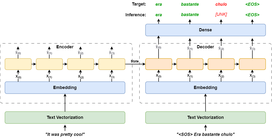
Implement an encoder-decoder recurrent network from scratch
Originally appeared here:
Keras 3.0 Tutorial: End-to-End Deep Learning Project Guide
Go Here to Read this Fast! Keras 3.0 Tutorial: End-to-End Deep Learning Project Guide

Implement an encoder-decoder recurrent network from scratch
Originally appeared here:
Keras 3.0 Tutorial: End-to-End Deep Learning Project Guide
Go Here to Read this Fast! Keras 3.0 Tutorial: End-to-End Deep Learning Project Guide
How physics principles give us deeper insights into our data
Originally appeared here:
The Physics Behind Data

With the growing number of embedding models available, choosing the right one for your machine learning applications can be challenging. Fortunately, the MTEB leaderboard provides a comprehensive range of ranking metrics for various natural language processing tasks.
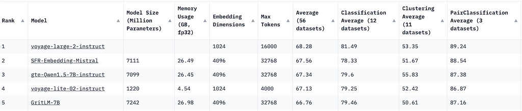
When you visit the site, you’ll notice that the top five embedding models are Generative Pre-trained Transformers (GPTs). This might lead you to think that GPT models are the best for embeddings. But is this really true? Let’s conduct an experiment to find out.
Embeddings are tensor representation of texts, that converts text token IDs and projects them into a tensor space.
By inputting text into a neural network model and performing a forward pass, you can obtain embedding vectors. However, the actual process is a bit more complex. Let’s break it down step by step:
In the first step, I am going to use a tokenizer to achieve it. model_inputs is the tensor representation of the text content, “some questions” .
from transformers import AutoModelForCausalLM, AutoTokenizer

tokenizer = AutoTokenizer.from_pretrained(
"mistralai/Mistral-7B-Instruct-v0.1"
)

messages = [
        {
            "role": "user",
            "content": "some questions",
        },
]

encodeds = tokenizer.apply_chat_template(messages, return_tensors="pt")
model_inputs = encodeds.to("cuda")
The second step is straightforward, passing the model_inputs into a neural network. The logits of generated tokens can be accessed via .logits .
import torch

with torch.no_grad():
  return model(model_inputs).logits
The third step is a bit tricky. GPT models are decoder-only, and their token generation is autoregressive. In simple terms, the last token of a completed sentence has seen all the preceding tokens in the sentence. Therefore, the output of the last token contains all the affinity scores (attentions) from the preceding tokens.
Bingo! You are most interested in the last token because of the attention mechanism in the transformers.
The output dimension of the GPTs implemented in Hugging Face is (batch size, input token size, number of vocabulary). To get the last token output of all the batches, I can perform a tensor slice.
import torch
with torch.no_grad():
  return model(model_inputs).logits[:, -1, :]
To measure the quality of these GPT embeddings, you can use cosine similarity. The higher the cosine similarity, the closer the semantic meaning of the sentences.
import torch
def compute_cosine_similarity(input1, input2):
    cos = torch.nn.CosineSimilarity(dim=1, eps=1e-6)
    return cos(input1, input2)
Let’s create some util functions that allows us to loop through list of question and answer pairs and see the result. Mistral 7b v0.1 instruct , one of the great open-sourced models, is used for this experiment.
from transformers import AutoTokenizer, AutoModelForCausalLM
from torch.distributions import Categorical
import torch
from termcolor import colored


model = AutoModelForCausalLM.from_pretrained(
  "mistralai/Mistral-7B-Instruct-v0.1"
)

tokenizer = AutoTokenizer.from_pretrained(
  "mistralai/Mistral-7B-Instruct-v0.1"
)

def generate_last_token_embeddings(question, max_new_tokens=30):
    messages = [
        {
            "role": "user",
            "content": question,
        },
    ]
    encodeds = tokenizer.apply_chat_template(messages, return_tensors="pt")
    model_inputs = encodeds.to("cuda")
    with torch.no_grad():
        return model(model_inputs).logits[:, -1, :]


def get_similarities(q_batch, a_batch):
    for q in q_batch:
        for a in a_batch:
            q_emb, a_emd = generate_last_token_embeddings(q), generate_last_token_embeddings(a),
            similarity = compute_cosine_similarity(q_emb, a_emd)
            print(colored(f"question: {q} and ans: {a}", "green"))
            print(colored(f"result: {similarity}", "blue"))

q = ["Where is the headquarter of OpenAI?",
    "What is GPU?"]
a = ["OpenAI is based at San Francisco.",
     "A graphics processing unit (GPU) is an electronic circuit that can perform mathematical calculations quickly",
    ]
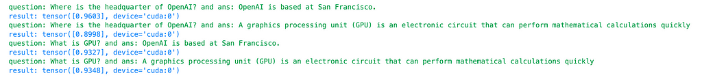
For the first question and answer pair:
For the second question and answer pair:
For an irrelevant pair:
For the worst pair:
These results suggest that using GPT models, in this case, the mistral 7b instruct v0.1, as embedding models may not yield great results in terms of distinguishing between relevant and irrelevant pairs. But why are GPT models still among the top 5 embedding models?
tokenizer = AutoTokenizer.from_pretrained("intfloat/e5-mistral-7b-instruct")
model = AutoModelForCausalLM.from_pretrained(
  "intfloat/e5-mistral-7b-instruct"
)
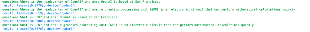
Repeating the same evaluation procedure with a different model, e5-mistral-7b-instruct, which is one of the top open-sourced models from the MTEB leaderboard and fine-tuned from mistral 7b instruct, I discover that the cosine similarity for the relevant question and pairs are 0.88 and 0.84 for OpenAI and GPU questions, respectively. For the irrelevant question and answer pairs, the similarity drops to 0.56 and 0.67. This findings suggests e5-mistral-7b-instruct is a much-improved model for embeddings. What makes such an improvement?
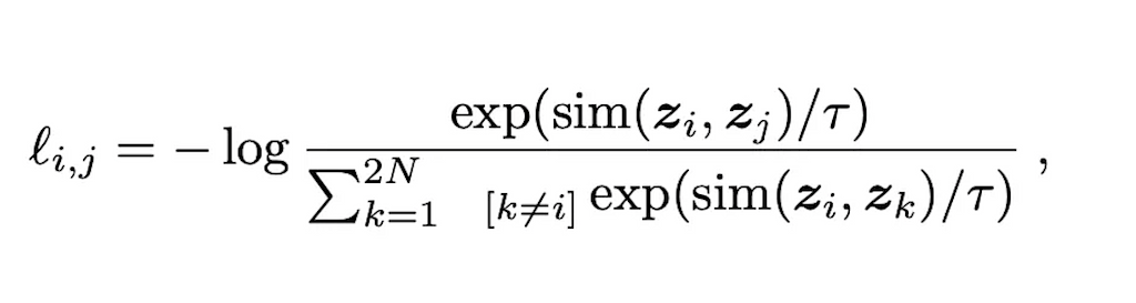
Delving into the paper behind e5-mistral-7b-instruct, the key is the use of contrastive loss to further fine tune the mistral model.
Unlike GPTs that are trained or further fine-tuned using cross-entropy loss of predicted tokens and labeled tokens, contrastive loss aims to maximize the distance between negative pairs and minimize the distance between the positive pairs.
This blog post covers this concept in greater details. The sim function calculates the cosine distance between two vectors. For contrastive loss, the denominators represent the cosine distance between positive examples and negative examples. The rationale behind contrastive loss is that we want similar vectors to be as close to 1 as possible, since log(1) = 0 represents the optimal loss.
In this post, I have highlighted a common pitfall of using GPTs as embedding models without fine-tuning. My evaluation suggests that fine-tuning GPTs with contrastive loss, the embeddings can be more meaningful and discriminative. By understanding the strengths and limitations of GPT models, and leveraging customized loss like contrastive loss, you can make more informed decisions when selecting and utilizing embedding models for your machine learning projects. I hope this post helps you choose GPTs models wisely for your applications and look forward to hearing your feedback! 🙂
Are GPTs Good Embedding Models was originally published in Towards Data Science on Medium, where people are continuing the conversation by highlighting and responding to this story.
Originally appeared here:
Are GPTs Good Embedding Models

Demystifying the term “accuracy” in Data Science and Artificial Intelligence
Originally appeared here:
Please Make this AI Less Accurate
Go Here to Read this Fast! Please Make this AI Less Accurate
Let’s learn how to identify and deal with the common causes of data leakage in ML models
Originally appeared here:
Common Causes of Data Leakage and how to Spot Them
Go Here to Read this Fast! Common Causes of Data Leakage and how to Spot Them


Originally appeared here:
Mixtral 8x22B is now available in Amazon SageMaker JumpStart
Go Here to Read this Fast! Mixtral 8x22B is now available in Amazon SageMaker JumpStart


Originally appeared here:
Building Generative AI prompt chaining workflows with human in the loop
Go Here to Read this Fast! Building Generative AI prompt chaining workflows with human in the loop

You must have heard the saying “garbage in, garbage out.” This saying is indeed applicable when training machine learning models. If we train machine learning models using irrelevant data, even the best machine learning algorithms won’t help much. Conversely, using well-engineered meaningful features can achieve superior performance even with a simple machine learning algorithm. So, then, how can we create these meaningful features that will maximize our model’s performance? The answer is feature engineering. Working on feature engineering is especially important when working with traditional machine learning algorithms, such as regressions, decision trees, support vector machines, and others that require numeric inputs. However, creating these numeric inputs is not just about data skills. It’s a process that demands creativity and domain knowledge and has as much art as science.
Broadly speaking, we can divide feature engineering into two components: 1) creating new features and 2) processing these features to make them work optimally with the machine learning algorithm under consideration. In this article, we will discuss these two components of feature engineering for cross-sectional, structured, non-NLP datasets.
Raw data gathering can be exhausting, and by the end of this task, we might be too tired to invest more time and energy in creating additional features. But this is where we must resist the temptation of diving straight into model training. I promise you that it will be well worth it! At this junction, we should pause and ask ourselves, “If I were to make the predictions manually based on my domain knowledge, what features would have helped me do a good job?” Asking this question may open up possibilities for crafting new meaningful features that our model might have missed otherwise. Once we have considered what additional features we could benefit from, we can leverage the techniques below to create new features from the raw data.
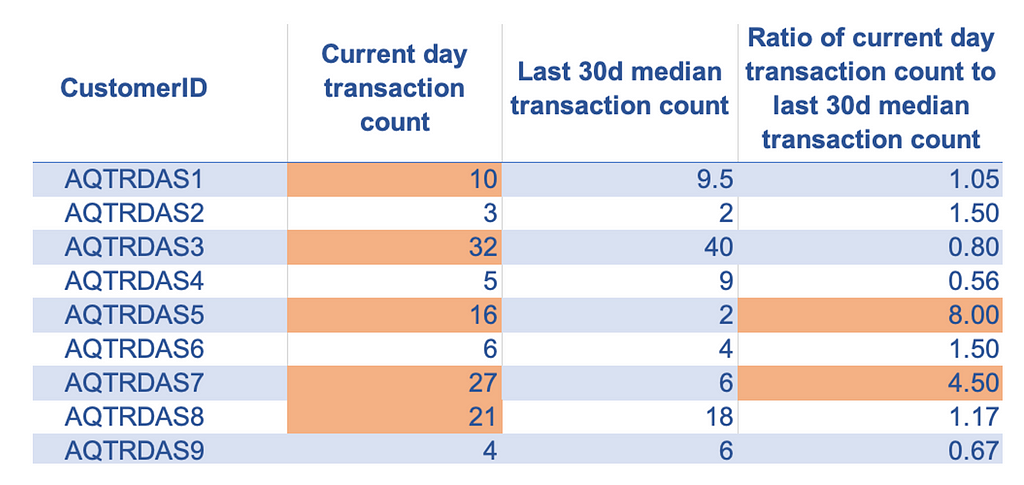
As the name suggests, this technique helps us combine multiple data points to create a more holistic view. We typically apply aggregations on continuous numeric data using standard functions like count, sum, average, minimum, maximum, percentile, standard deviation, and coefficient of variation. Each function can capture different elements of information, and the best function to use depends on the specific use case. Often, we can apply aggregation over a particular time or event window that is meaningful in the context of that problem.
Let’s take an example where we want to predict whether a given credit card transaction is fraudulent. For this use case, we can undoubtedly use transaction-specific features, but alongside those features, we can also benefit from creating aggregated customer-level features like:
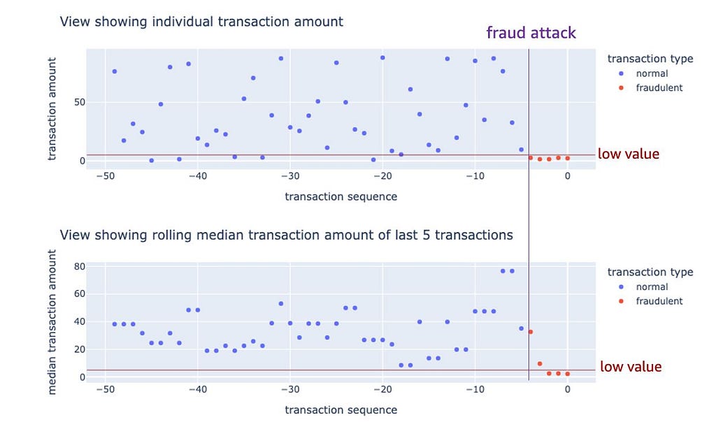
In many types of problems, change in a set pattern is a valuable signal for prediction or anomaly detection. Differences and ratios are effective techniques for representing changes in numeric features. Just like aggregation, we can also apply these techniques over a meaningful time window in the context of that problem.
Examples:
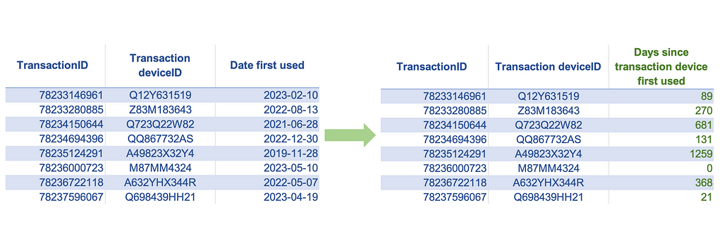
We can use the age calculation technique to convert the date or timestamp features to numeric features by taking the difference between two timestamps or dates. We can also use this technique to convert certain non-numeric features into meaningful numeric features if the tenure associated with the feature values can be a valuable signal for prediction.
Examples:
Indicator or Boolean features have binary values {1, 0} or {True, False}. Indicator features are very common and are used to represent various types of binary information. In some cases, we may already have such binary features in numeric form, while in other instances, they may have non-numeric values. To use the non-numeric binary features for model training, all we have to do is map them to numeric values.
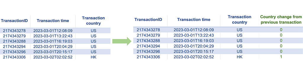
Looking beyond these common occurrences and uses of indicator features, we can leverage indicator encoding as a tool to represent a comparison between non-numeric data points. This attribute makes it particularly powerful as it creates a way for us to measure the changes in non-numeric features.
Examples:
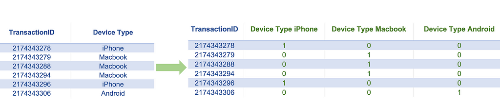
This technique can be applied if our feature data is in categorical form, either numeric or non-numeric. The numeric-categorical form refers to numeric data containing non-continuous or non-measurement data, such as geographical region codes, store IDs, and other such types of data. One hot encoding technique can convert such features into a set of indicator features that we can use in training machine learning models. Applying one hot encoding on a categorical feature will create one new binary feature for every category in that categorical variable. Since the number of new features increases as the number of categories increases, this technique is suitable for features with a low number of categories, especially if we have a smaller dataset. One of the standard rules of thumb suggests applying this technique if we have at least ten records per category.
Examples:
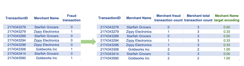
This technique is applied to the same type of features that we would apply the one-hot encoding to but has some advantages and disadvantages over one-hot encoding. When the number of categories is high (high cardinality), using one-hot encoding will undesirably increase the number of features, which may lead to model overfitting. Target encoding can be an effective technique in such cases, provided we are working on a supervised learning problem. It is a technique that maps each category value to the expected value of the target for that category. If working with a regression problem with a continuous target, this calculation maps the category to the mean target value for that category. In the case of a classification problem with a binary target, target encoding will map the category to the positive event probability of that category. Unlike one-hot encoding, this technique has the advantage of not increasing the number of features. A downside of this technique is that it can only be applied to supervised learning problems. Applying this technique may also make the model susceptible to overfitting, particularly if the number of observations in some categories is low.
Examples:
Once we have created the new features from the raw data, the next step is to process them for optimal model performance. We accomplish this though feature processing as discussed in the next section.
Feature processing refers to series of data processing steps that ensure that the machine learning models fit the data as intended. While some of these processing steps are required when using certain machine learning algorithms, others ensure that we strike a good working chemistry between the features and the machine learning algorithm under consideration. In this section, let’s discuss some common feature processing steps and why we need them.
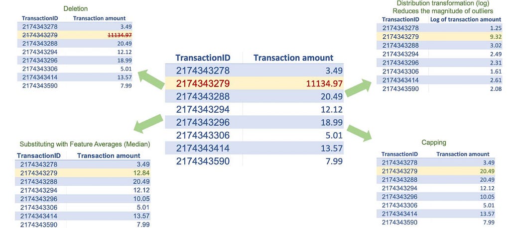
Several machine learning algorithms, especially parametric ones such as regression models, are severely impacted by outliers. These machine learning algorithms attempt to accommodate outliers, severely affecting the model parameters and compromising overall performance. To treat the outliers, we must first identify them. We can detect outliers for a specific feature by applying certain rules of thumb, such as having an absolute value greater than the mean plus three standard deviations or a value outside the nearest whisker value (nearest quartile value plus 1.5 times the interquartile range value). Once we have identified the outliers in a specific feature, we can use some of the techniques below to treat outliers:
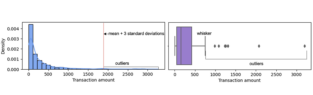
Note that there are techniques to detect observations that are multivariate outliers (outliers with respect to multiple features), but they are more complex and generally do not add much value in terms of machine learning model training. Also note that outliers are not a concern when working with most non-parametric machine learning models like support vector machines and tree-based algorithms like decision trees, random forests, and XGBoost.
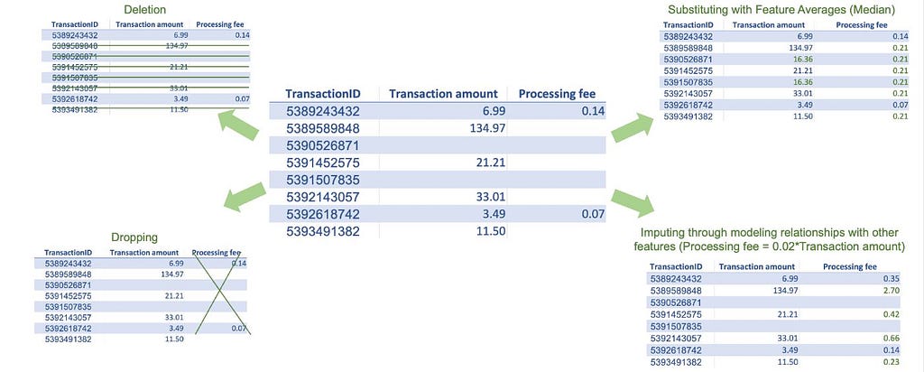
Missing data is very common in real-world datasets. Most traditional machine learning algorithms, except a few like XGBoost, don’t allow missing values in training datasets. Thus, fixing missing values is one of the routine tasks in machine learning modeling. There are several techniques to treat missing values; however, before implementing any technique, it is important to understand the cause of the missing data or, at the very least, know if the data is missing at random. If the data is not missing at random, meaning certain subgroups are more likely to have missing data, imputing values for those might be difficult, especially if there is little to no data available. If the data is missing at random, we can use some of the common treatment techniques described below. They all have pros and cons, and it’s up to us to decide what method best suits our use case.
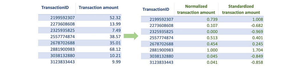
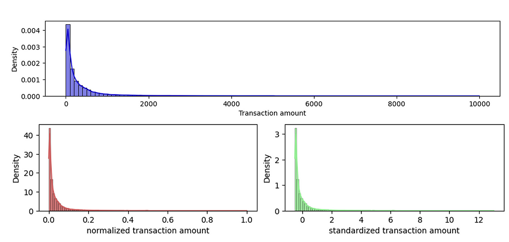
Often, features that we use in machine learning models have different ranges. If we use them without scaling, the features with large absolute values will dominate the prediction outcome. Instead, to give each feature a fair opportunity to contribute to the prediction outcome, we must bring all features on the same scale. The two most common scaling techniques are:
Note that tree-based algorithms like decision trees, random forest, XGBoost, and others can work with unscaled data and do not need scaling when using these algorithms.
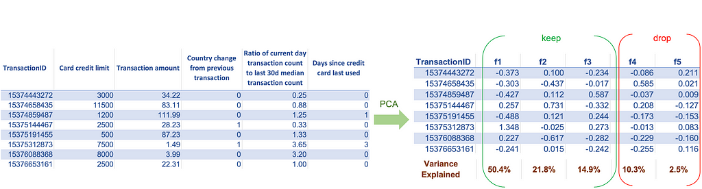
Today, we have enormous data, and we can build a vast collection of features to train our models. For most algorithms, having more features is good since it provides more options to improve the model performance. However, this is not true for all algorithms. Algorithms based on distance metrics suffer from the curse of dimensionality — as the number of features increases substantially, the distance value between the two observations becomes meaningless. Thus, to use algorithms that rely on distance metrics, we should ensure that we are not using a large number of features. If our dataset has a large number of features and if we don’t know which ones to keep and which to discard, we can use techniques like Principal component analysis (PCA). PCA transforms the set of old features into a set of new features. It creates new features such that the one with the highest eigenvalues captures most of the information from the old features. We can then keep only the top few new features and discard the remaining ones.
Other statistical techniques, such as association analysis and feature selection algorithms, can be used in supervised learning problems to reduce the number of features. However, they generally do not capture the same level of information that PCA does with the same number of features.
This step is an exception because it only applies to the target and not to the features. Also, most machine learning algorithms don’t have any restrictions on the target’s distribution, but certain ones like linear regression, require that the target to be distributed normally. Linear regression assumes that the error values are symmetric and concentrated around zero for all the data points (just like the shape of the normal distribution), and a normally distributed target variable ensures that this assumption is met. We can understand our target’s distribution by plotting a histogram. Statistical tests like the Shapiro-Wilk test tell us about the normality by testing this hypothesis. In case our target is not normally distributed, we can try out various transformations such as log transform, square transform, square root transform, and others to check which transforms make the target distribution normal. There is also a Box-Cox transformation that tries out multiple parameter values, and we can choose the one that best transforms our target’s distribution to normal.

Note: While we can implement the feature processing steps in features in any order, we must thoroughly consider the sequence of their application. For example, missing value treatment using value mean substitution can be implemented before or after outlier detection. However, the mean value used for substitution may differ depending on whether we treat the missing values before or after the outlier treatment. The feature processing sequence outlined in this article treats the issues in the order of the impact they can have on the successive processing steps. Thus, following this sequence should generally be effective for addressing most problems.
As mentioned in the introduction, feature engineering is a dimension of machine learning that allows us to control the model’s performance to an exceptional degree. To exploit feature engineering to its potential, we learned various techniques in this article to create new features and process them to work optimally with machine learning models. No matter what feature engineering principles and techniques from this article you choose to use, the important message here is to understand that machine learning is not just about asking the algorithm to figure out the patterns. It is about us enabling the algorithm to do its job effectively by providing the kind of data it needs.
Unless otherwise noted, all images are by the author.
Feature Engineering for Machine Learning was originally published in Towards Data Science on Medium, where people are continuing the conversation by highlighting and responding to this story.
Originally appeared here:
Feature Engineering for Machine Learning
Go Here to Read this Fast! Feature Engineering for Machine Learning

An explanation of the backpropagation through time algorithm
Originally appeared here:
Backpropagation Through Time — How RNNs Learn
Go Here to Read this Fast! Backpropagation Through Time — How RNNs Learn