Originally appeared here:
Introducing Time Series in pandas
Go Here to Read this Fast! Introducing Time Series in pandas


Decomposition of an integer object in Python for memory consumption
Originally appeared here:
Why does an Integer Need 28 Bytes in Python?
Go Here to Read this Fast! Why does an Integer Need 28 Bytes in Python?
Improve Python code for data science with simple, readable and performant enumerations.
Originally appeared here:
A Guide to Powerful Python Enumerations
Go Here to Read this Fast! A Guide to Powerful Python Enumerations

Intuition, algorithm and code for using ALEs to explain machine learning models
Originally appeared here:
Deep Dive on Accumulated Local Effect Plots (ALEs) with Python
Go Here to Read this Fast! Deep Dive on Accumulated Local Effect Plots (ALEs) with Python


Large Language Models are amazing, but for many production problems, simpler techniques are faster, cheaper, and just as…
Originally appeared here:
Yes, you still need old-school NLP skills in “the age of ChatGPT”
Go Here to Read this Fast! Yes, you still need old-school NLP skills in “the age of ChatGPT”

Part 4 in the “LLMs from Scratch” series — a complete guide to understanding and building Large Language Models. If you are interested in learning more about how these models work I encourage you to read:
Bidirectional Encoder Representations from Transformers (BERT) is a Large Language Model (LLM) developed by Google AI Language which has made significant advancements in the field of Natural Language Processing (NLP). Many models in recent years have been inspired by or are direct improvements to BERT, such as RoBERTa, ALBERT, and DistilBERT to name a few. The original BERT model was released shortly after OpenAI’s Generative Pre-trained Transformer (GPT), with both building on the work of the Transformer architecture proposed the year prior. While GPT focused on Natural Language Generation (NLG), BERT prioritised Natural Language Understanding (NLU). These two developments reshaped the landscape of NLP, cementing themselves as notable milestones in the progression of machine learning.
The following article will explore the history of BERT, and detail the landscape at the time of its creation. This will give a complete picture of not only the architectural decisions made by the paper’s authors, but also an understanding of how to train and fine-tune BERT for use in industry and hobbyist applications. We will step through a detailed look at the architecture with diagrams and write code from scratch to fine-tune BERT on a sentiment analysis task.
1 — History and Key Features of BERT
2 — Architecture and Pre-training Objectives
3 — Fine-Tuning BERT for Sentiment Analysis
The BERT model can be defined by four main features:
Each of these features were design choices made by the paper’s authors and can be understood by considering the time in which the model was created. The following section will walk through each of these features and show how they were either inspired by BERT’s contemporaries (the Transformer and GPT) or intended as an improvement to them.
The debut of the Transformer in 2017 kickstarted a race to produce new models that built on its innovative design. OpenAI struck first in June 2018, creating GPT: a decoder-only model that excelled in NLG, eventually going on to power ChatGPT in later iterations. Google responded by releasing BERT four months later: an encoder-only model designed for NLU. Both of these architectures can produce very capable models, but the tasks they are able to perform are slightly different. An overview of each architecture is given below.
Decoder-Only Models:
Encoder-Only Models:
“sub-optimal for sentence-level tasks, and could be very harmful when applying finetuning based approaches to token-level tasks such as question answering” [1]
Note: It is technically possible to generate text with BERT, but as we will see, this is not what the architecture was intended for, and the results do not rival decoder-only models in any way.
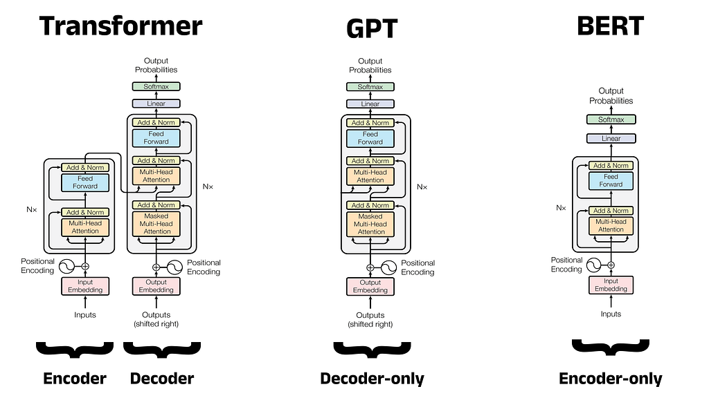
Architecture Diagrams for the Transformer, GPT, and BERT:
Below is an architecture diagram for the three models we have discussed so far. This has been created by adapting the architecture diagram from the original Transformer paper “Attention is All You Need” [2]. The number of encoder or decoder blocks for the model is denoted by N. In the original Transformer, N is equal to 6 for the encoder and 6 for the decoder, since these are both made up of six encoder and decoder blocks stacked together respectively.
GPT influenced the development of BERT in several ways. Not only was the model the first decoder-only Transformer derivative, but GPT also popularised model pre-training. Pre-training involves training a single large model to acquire a broad understanding of language (encompassing aspects such as word usage and grammatical patterns) in order to produce a task-agnostic foundational model. In the diagrams above, the foundational model is made up of the components below the linear layer (shown in purple). Once trained, copies of this foundational model can be fine-tuned to address specific tasks. Fine-tuning involves training only the linear layer: a small feedforward neural network, often called a classification head or just a head. The weights and biases in the remainder of the model (that is, the foundational portion) remained unchanged, or frozen.
Analogy:
To construct a brief analogy, consider a sentiment analysis task. Here, the goal is to classify text as either positive or negative based on the sentiment portrayed. For example, in some movie reviews, text such as I loved this movie would be classified as positive and text such as I hated this movie would be classified as negative. In the traditional approach to language modelling, you would likely train a new architecture from scratch specifically for this one task. You could think of this as teaching someone the English language from scratch by showing them movie reviews until eventually they are able to classify the sentiment found within them. This of course, would be slow, expensive, and require many training examples. Moreover, the resulting classifier would still only be proficient in this one task. In the pre-training approach, you take a generic model and fine-tune it for sentiment analysis. You can think of this as taking someone who is already fluent in English and simply showing them a small number of movie reviews to familiarise them with the current task. Hopefully, it is intuitive that the second approach is much more efficient.
Earlier Attempts at Pre-training:
The concept of pre-training was not invented by OpenAI, and had been explored by other researchers in the years prior. One notable example is the ELMo model (Embeddings from Language Models), developed by researchers at the Allen Institute [3]. Despite these earlier attempts, no other researchers were able to demonstrate the effectiveness of pre-training as convincingly as OpenAI in their seminal paper. In their own words, the team found that their
“task-agnostic model outperforms discriminatively trained models that use architectures specifically crafted for each task, significantly improving upon the state of the art” [4].
This revelation firmly established the pre-training paradigm as the dominant approach to language modelling moving forward. In line with this trend, the BERT authors also fully adopted the pre-trained approach.
Benefits of Fine-tuning:
Fine-tuning has become commonplace today, making it easy to overlook how recent it was that this approach rose to prominence. Prior to 2018, it was typical for a new model architecture to be introduced for each distinct NLP task. Transitioning to pre-training not only drastically decreased the training time and compute cost needed to develop a model, but also reduced the volume of training data required. Rather than completely redesigning and retraining a language model from scratch, a generic model like GPT could be fine-tuned with a small amount of task-specific data in a fraction of the time. Depending on the task, the classification head can be changed to contain a different number of output neurons. This is useful for classification tasks such as sentiment analysis. For example, if the desired output of a BERT model is to predict whether a review is positive or negative, the head can be changed to feature two output neurons. The activation of each indicates the probability of the review being positive or negative respectively. For a multi-class classification task with 10 classes, the head can be changed to have 10 neurons in the output layer, and so on. This makes BERT more versatile, allowing the foundational model to be used for various downstream tasks.
Fine-tuning in BERT:
BERT followed in the footsteps of GPT and also took this pre-training/fine-tuning approach. Google released two versions of BERT: Base and Large, offering users flexibility in model size based on hardware constraints. Both variants took around 4 days to pre-train on many TPUs (tensor processing units), with BERT Base trained on 16 TPUs and BERT Large trained on 64 TPUs. For most researchers, hobbyists, and industry practitioners, this level of training would not be feasible. Hence, the idea of spending only a few hours fine-tuning a foundational model on a particular task remains a much more appealing alternative. The original BERT architecture has undergone thousands of fine-tuning iterations across various tasks and datasets, many of which are publicly accessible for download on platforms like Hugging Face [5].
As a language model, BERT predicts the probability of observing certain words given that prior words have been observed. This fundamental aspect is shared by all language models, irrespective of their architecture and intended task. However, it’s the utilisation of these probabilities that gives the model its task-specific behaviour. For example, GPT is trained to predict the next most probable word in a sequence. That is, the model predicts the next word, given that the previous words have been observed. Other models might be trained on sentiment analysis, predicting the sentiment of an input sequence using a textual label such as positive or negative, and so on. Making any meaningful predictions about text requires the surrounding context to be understood, especially in NLU tasks. BERT ensures good understanding through one of its key properties: bidirectionality.
Bidirectionality is perhaps BERT’s most significant feature and is pivotal to its high performance in NLU tasks, as well as being the driving reason behind the model’s encoder-only architecture. While the self-attention mechanism of Transformer encoders calculates bidirectional context, the same cannot be said for decoders which produce unidirectional context. The BERT authors argued that this lack of bidirectionality in GPT prevents it from achieving the same depth of language representation as BERT.
Defining Bidirectionality:
But what exactly does “bidirectional” context mean? Here, bidirectional denotes that each word in the input sequence can gain context from both preceding and succeeding words (called the left context and right context respectively). In technical terms, we say that the attention mechanism can attend to the preceding and subsequent tokens for each word. To break this down, recall that BERT only makes predictions about words within an input sequence, and does not generate new sequences like GPT. Therefore, when BERT predicts a word within the input sequence, it can incorporate contextual clues from all the surrounding words. This gives context in both directions, helping BERT to make more informed predictions.
Contrast this with decoder-only models like GPT, where the objective is to predict new words one at a time to generate an output sequence. Each predicted word can only leverage the context provided by preceding words (left context) as the subsequent words (right context) have not yet been generated. Therefore, these models are called unidirectional.
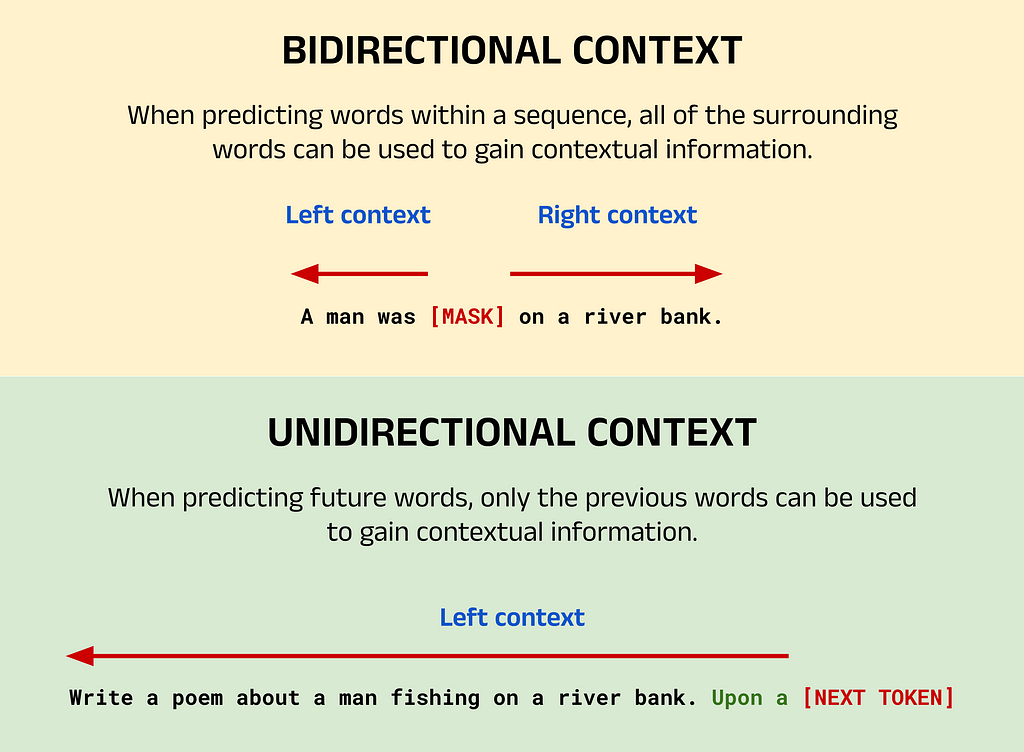
Image Breakdown:
The image above shows an example of a typical BERT task using bidirectional context, and a typical GPT task using unidirectional context. For BERT, the task here is to predict the masked word indicated by [MASK]. Since this word has words to both the left and right, the words from either side can be used to provide context. If you, as a human, read this sentence with only the left or right context, you would probably struggle to predict the masked word yourself. However, with bidirectional context it becomes much more likely to guess that the masked word is fishing.
For GPT, the goal is to perform the classic NTP task. In this case, the objective is to generate a new sequence based on the context provided by the input sequence and the words already generated in the output. Given that the input sequence instructs the model to write a poem and the words generated so far are Upon a, you might predict that the next word is river followed by bank. With many potential candidate words, GPT (as a language model) calculates the likelihood of each word in its vocabulary appearing next and selects one of the most probable words based on its training data.
As a bidirectional model, BERT suffers from two major drawbacks:
Increased Training Time:
Bidirectionality in Transformer-based models was proposed as a direct improvement over the left-to-right context models prevalent at the time. The idea was that GPT could only gain contextual information about input sequences in a unidirectional manner and therefore lacked a complete grasp of the causal links between words. Bidirectional models, however, offer a broader understanding of the causal connections between words and so can potentially see better results on NLU tasks. Though bidirectional models had been explored in the past, their success was limited, as seen with bidirectional RNNs in the late 1990s [6]. Typically, these models demand more computational resources for training, so for the same computational power you could train a larger unidirectional model.
Poor Performance in Language Generation:
BERT was specifically designed to solve NLU tasks, opting to trade decoders and the ability to generate new sequences for encoders and the ability to develop rich understandings of input sequences. As a result, BERT is best suited to a subset of NLP tasks like NER, sentiment analysis and so on. Notably, BERT doesn’t accept prompts but rather processes sequences to formulate predictions about. While BERT can technically produce new output sequences, it is important to recognise the design differences between LLMs as we might think of them in the post-ChatGPT era, and the reality of BERT’s design.
Training a bidirectional model requires tasks that allow both the left and right context to be used in making predictions. Therefore, the authors carefully constructed two pre-training objectives to build up BERT’s understanding of language. These were: the Masked Language Model task (MLM), and the Next Sentence Prediction task (NSP). The training data for each was constructed from a scrape of all the English Wikipedia articles available at the time (2,500 million words), and an additional 11,038 books from the BookCorpus dataset (800 million words) [7]. The raw data was first preprocessed according to the specific tasks however, as described below.
Overview of MLM:
The Masked Language Modelling task was created to directly address the need for training a bidirectional model. To do so, the model must be trained to use both the left context and right context of an input sequence to make a prediction. This is achieved by randomly masking 15% of the words in the training data, and training BERT to predict the missing word. In the input sequence, the masked word is replaced with the [MASK] token. For example, consider that the sentence A man was fishing on the river exists in the raw training data found in the book corpus. When converting the raw text into training data for the MLM task, the word fishing might be randomly masked and replaced with the [MASK] token, giving the training input A man was [MASK] on the river with target fishing. Therefore, the goal of BERT is to predict the single missing word fishing, and not regenerate the input sequence with the missing word filled in. The masking process can be repeated for all the possible input sequences (e.g. sentences) when building up the training data for the MLM task. This task had existed previously in linguistics literature, and is referred to as the Cloze task [8]. However, in machine learning contexts, it is commonly referred to as MLM due to the popularity of BERT.
Mitigating Mismatches Between Pre-training and Fine-tuning:
The authors noted however, that since the [MASK] token will only ever appear in the training data and not in live data (at inference time), there would be a mismatch between pre-training and fine-tuning. To mitigate this, not all masked words are replaced with the [MASK] token. Instead, the authors state that:
The training data generator chooses 15% of the token positions at random for prediction. If the i-th token is chosen, we replace the i-th token with (1) the [MASK] token 80% of the time (2) a random token 10% of the time (3) the unchanged i-th token 10% of the time.
Calculating the Error Between the Predicted Word and the Target Word:
BERT will take in an input sequence of a maximum of 512 tokens for both BERT Base and BERT Large. If fewer than the maximum number of tokens are found in the sequence, then padding will be added using [PAD] tokens to reach the maximum count of 512. The number of output tokens will also be exactly equal to the number of input tokens. If a masked token exists at position i in the input sequence, BERT’s prediction will lie at position i in the output sequence. All other tokens will be ignored for the purposes of training, and so updates to the models weights and biases will be calculated based on the error between the predicted token at position i, and the target token. The error is calculated using a loss function, which is typically the Cross Entropy Loss (Negative Log Likelihood) function, as we will see later.
Overview:
The second of BERT’s pre-training tasks is Next Sentence Prediction, in which the goal is to classify if one segment (typically a sentence) logically follows on from another. The choice of NSP as a pre-training task was made specifically to complement MLM and enhance BERT’s NLU capabilities, with the authors stating:
Many important downstream tasks such as Question Answering (QA) and Natural Language Inference (NLI) are based on understanding the relationship between two sentences, which is not directly captured by language modeling.
By pre-training for NSP, BERT is able to develop an understanding of flow between sentences in prose text — an ability that is useful for a wide range of NLU problems, such as:
Implementing NSP in BERT:
The input for NSP consists of the first and second segments (denoted A and B) separated by a [SEP] token with a second [SEP] token at the end. BERT actually expects at least one [SEP] token per input sequence to denote the end of the sequence, regardless of whether NSP is being performed or not. For this reason, the WordPiece tokenizer will append one of these tokens to the end of inputs for the MLM task as well as any other non-NSP task that do not feature one. NSP forms a classification problem, where the output corresponds to IsNext when segment A logically follows segment B, and NotNext when it does not. Training data can be easily generated from any monolingual corpus by selecting sentences with their next sentence 50% of the time, and a random sentence for the remaining 50% of sentences.
2.4 — Input Embeddings in BERT
The input embedding process for BERT is made up of three stages: positional encoding, segment embedding, and token embedding (as shown in the diagram below).
Positional Encoding:
Just as with the Transformer model, positional information is injected into the embedding for each token. Unlike the Transformer however, the positional encodings in BERT are fixed and not generated by a function. This means that BERT is restricted to 512 tokens in its input sequence for both BERT Base and BERT Large.
Segment Embedding:
Vectors encoding the segment that each token belongs to are also added. For the MLM pre-training task or any other non-NSP task (which feature only one [SEP]) token, all tokens in the input are considered to belong to segment A. For NSP tasks, all tokens after the second [SEP] are denoted as segment B.
Token Embedding:
As with the original Transformer, the learned embedding for each token is then added to its positional and segment vectors to create the final embedding that will be passed to the self-attention mechanisms in BERT to add contextual information.
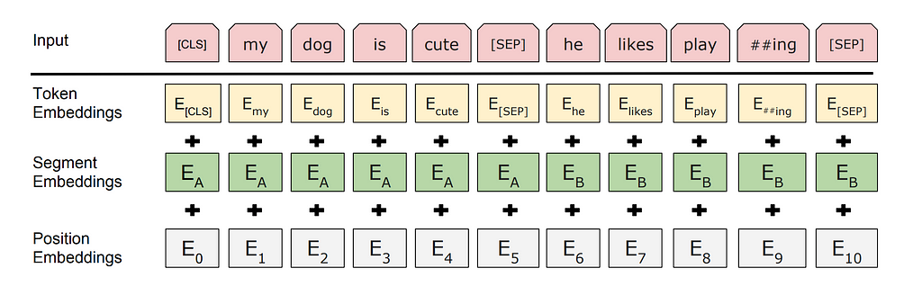
In the image above, you may have noted that the input sequence has been prepended with a [CLS] (classification) token. This token is added to encapsulate a summary of the semantic meaning of the entire input sequence, and helps BERT to perform classification tasks. For example, in the sentiment analysis task, the [CLS] token in the final layer can be analysed to extract a prediction for whether the sentiment of the input sequence is positive or negative. [CLS] and [PAD] etc are examples of BERT’s special tokens. It’s important to note here that this is a BERT-specific feature, and so you should not expect to see these special tokens in models such as GPT. In total, BERT has five special tokens. A summary is provided below:
BERT Base and BERT Large are very similar from an architecture point-of-view, as you might expect. They both use the WordPiece tokenizer (and hence expect the same special tokens described earlier), and both have a maximum sequence length of 512 tokens. They also both use 768 embedding dimensions, which corresponds to the size of the learned vector representations for each token in the model’s vocabulary (d_model = 768). You may notice that this is larger than the original Transformer, which used 512 embedding dimensions (d_model = 512). The vocabulary size for BERT is 30,522, with approximately 1,000 of those tokens left as “unused”. The unused tokens are intentionally left blank to allow users to add custom tokens without having to retrain the entire tokenizer. This is useful when working with domain-specific vocabulary, such as medical and legal terminology.
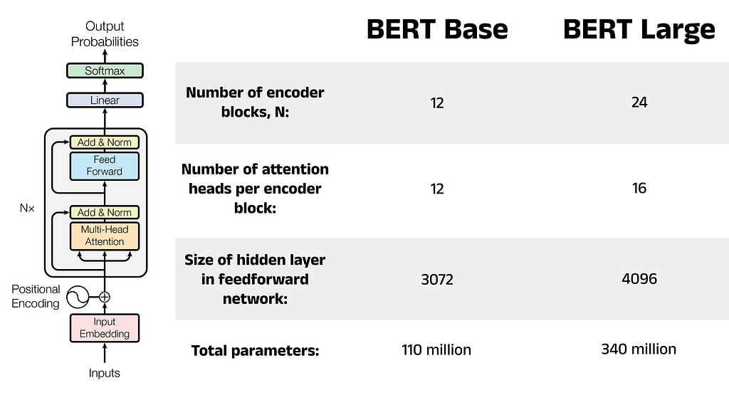
The two models mainly differ in four categories:
A comparison between BERT Base and BERT Large for each of these categories is shown in the image below.
This section covers a practical example of fine-tuning BERT in Python. The code takes the form of a task-agnostic fine-tuning pipeline, implemented in a Python class. We will then instantiate an object of this class and use it to fine-tune a BERT model on the sentiment analysis task. The class can be reused to fine-tune BERT on other tasks, such as Question Answering, Named Entity Recognition, and more. Sections 3.1 to 3.5 walk through the fine-tuning process, and Section 3.6 shows the full pipeline in its entirety.
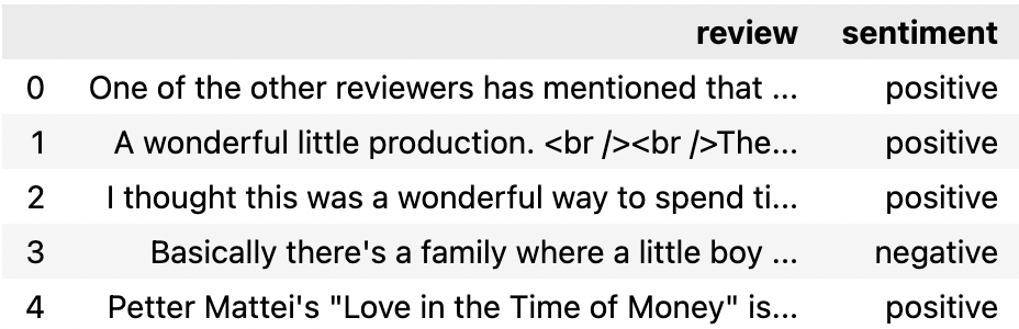
The first step in fine-tuning is to select a dataset that is suitable for the specific task. In this example, we will use a sentiment analysis dataset provided by Stanford University. This dataset contains 50,000 online movie reviews from the Internet Movie Database (IMDb), with each review labelled as either positive or negative. You can download the dataset directly from the Stanford University website, or you can create a notebook on Kaggle and compare your work with others.
import pandas as pd

df = pd.read_csv('IMDB Dataset.csv')
df.head()
Unlike earlier NLP models, Transformer-based models such as BERT require minimal preprocessing. Steps such as removing stop words and punctuation can prove counterproductive in some cases, since these elements provide BERT with valuable context for understanding the input sentences. Nevertheless, it is still important to inspect the text to check for any formatting issues or unwanted characters. Overall, the IMDb dataset is fairly clean. However, there appear to be some artefacts of the scraping process leftover, such as HTML break tags (<br />) and unnecessary whitespace, which should be removed.
# Remove the break tags (<br />)
df['review_cleaned'] = df['review'].apply(lambda x: x.replace('<br />', ''))

# Remove unnecessary whitespace
df['review_cleaned'] = df['review_cleaned'].replace('s+', ' ', regex=True)

# Compare 72 characters of the second review before and after cleaning
print('Before cleaning:')
print(df.iloc[1]['review'][0:72])

print('nAfter cleaning:')
print(df.iloc[1]['review_cleaned'][0:72])
Before cleaning:
A wonderful little production. <br /><br />The filming technique is very

After cleaning:
A wonderful little production. The filming technique is very unassuming-
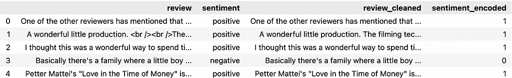
Encode the Sentiment:
The final step of the preprocessing is to encode the sentiment of each review as either 0 for negative or 1 for positive. These labels will be used to train the classification head later in the fine-tuning process.
df['sentiment_encoded'] = df['sentiment'].
    apply(lambda x: 0 if x == 'negative' else 1)
df.head()
Once preprocessed, the fine-tuning data can undergo tokenization. This process: splits the review text into individual tokens, adds the [CLS] and [SEP] special tokens, and handles padding. It’s important to select the appropriate tokenizer for the model, as different language models require different tokenization steps (e.g. GPT does not expect [CLS] and [SEP] tokens). We will use the BertTokenizer class from the Hugging Face transformers library, which is designed to be used with BERT-based models. For a more in-depth discussion of how tokenization works, see Part 1 of this series.
Tokenizer classes in the transformers library provide a simple way to create pre-trained tokenizer models with the from_pretrained method. To use this feature: import and instantiate a tokenizer class, call the from_pretrained method, and pass in a string with the name of a tokenizer model hosted on the Hugging Face model repository. Alternatively, you can pass in the path to a directory containing the vocabulary files required by the tokenizer [9]. For our example, we will use a pre-trained tokenizer from the model repository. There are four main options when working with BERT, each of which use the vocabulary from Google’s pre-trained tokenizers. These are:
Both BERT Base and BERT Large use the same vocabulary, and so there is actually no difference between bert-base-uncased and bert-large-uncased, nor is there a difference between bert-base-cased and bert-large-cased. This may not be the same for other models, so it is best to use the same tokenizer and model size if you are unsure.
When to Use cased vs uncased:
The decision between using cased and uncased depends on the nature of your dataset. The IMDb dataset contains text written by internet users who may be inconsistent with their use of capitalisation. For example, some users may omit capitalisation where it is expected, or use capitalisation for dramatic effect (to show excitement, frustration, etc). For this reason, we will choose to ignore case and use the bert-base-uncased tokenizer model.
Other situations may see a performance benefit by accounting for case. An example here may be in a Named Entity Recognition task, where the goal is to identify entities such as people, organisations, locations, etc in some input text. In this case, the presence of upper case letters can be extremely helpful in identifying if a word is someone’s name or a place, and so in this situation it may be more appropriate to choose bert-base-cased.
from transformers import BertTokenizer

tokenizer = BertTokenizer.from_pretrained('bert-base-uncased')
print(tokenizer)
BertTokenizer(
  name_or_path='bert-base-uncased',
  vocab_size=30522,
  model_max_length=512,
  is_fast=False,
  padding_side='right',
  truncation_side='right',
  special_tokens={
    'unk_token': '[UNK]',
    'sep_token': '[SEP]',
    'pad_token': '[PAD]',
    'cls_token': '[CLS]',
    'mask_token': '[MASK]'},
  clean_up_tokenization_spaces=True),

added_tokens_decoder={
  0: AddedToken(
    "[PAD]",
    rstrip=False,
    lstrip=False,
    single_word=False,
    normalized=False,
    special=True),

  100: AddedToken(
    "[UNK]",
    rstrip=False,
    lstrip=False,
    single_word=False,
    normalized=False,
    special=True),

  101: AddedToken(
    "[CLS]",
    rstrip=False,
    lstrip=False,
    single_word=False,
    normalized=False,
    special=True),

  102: AddedToken(
    "[SEP]",
    rstrip=False,
    lstrip=False,
    single_word=False,
    normalized=False,
    special=True),

  103: AddedToken(
    "[MASK]",
    rstrip=False,
    lstrip=False,
    single_word=False,
    normalized=False,
    special=True),
  }
Encoding Process: Converting Text to Tokens to Token IDs
Next, the tokenizer can be used to encode the cleaned fine-tuning data. This process will convert each review into a tensor of token IDs. For example, the review I liked this movie will be encoded by the following steps:
1. Convert the review to lower case (since we are using bert-base-uncased)
2. Break the review down into individual tokens according to the bert-base-uncased vocabulary: [‘i’, ‘liked’, ‘this’, ‘movie’]
2. Add the special tokens expected by BERT: [‘[CLS]’, ‘i’, ‘liked’, ‘this’, ‘movie’, ‘[SEP]’]
3. Convert the tokens to their token IDs, also according to the bert-base-uncased vocabulary (e.g. [CLS] -> 101, i -> 1045, etc)
The encode method of the BertTokenizer class encodes text using the above process, and can return the tensor of token IDs as PyTorch tensors, Tensorflow tensors, or NumPy arrays. The data type for the return tensor can be specified using the return_tensors argument, which takes the values: pt, tf, and np respectively.
Note: Token IDs are often called input IDs in Hugging Face, so you may see these terms used interchangeably.
# Encode a sample input sentence
sample_sentence = 'I liked this movie'
token_ids = tokenizer.encode(sample_sentence, return_tensors='np')[0]
print(f'Token IDs: {token_ids}')

# Convert the token IDs back to tokens to reveal the special tokens added
tokens = tokenizer.convert_ids_to_tokens(token_ids)
print(f'Tokens   : {tokens}')
Token IDs: [ 101 1045 4669 2023 3185  102]
Tokens   : ['[CLS]', 'i', 'liked', 'this', 'movie', '[SEP]']
Truncation and Padding:
Both BERT Base and BERT Large are designed to handle input sequences of exactly 512 tokens. But what do you do when your input sequence doesn’t fit this limit? The answer is truncation and padding! Truncation reduces the number of tokens by simply removing any tokens beyond a certain length. In the encode method, you can set truncation to True and specify a max_length argument to enforce a length limit on all encoded sequences. Several of the entries in this dataset exceed the 512 token limit, and so the max_length parameter here has been set to 512 to extract the most amount of text possible from all reviews. If no review exceeds 512 tokens, the max_length parameter can be left unset and it will default to the model’s maximum length. Alternatively, you can still enforce a maximum length which is less than 512 to reduce training time during fine-tuning, albeit at the expense of model performance. For reviews shorter than 512 tokens (which is the majority here), padding tokens are added to extend the encoded review to 512 tokens. This can be achieved by setting the padding parameter to max_length. Refer to the Hugging Face documentation for more details on the encode method [10].
review = df['review_cleaned'].iloc[0]

token_ids = tokenizer.encode(
    review,
    max_length = 512,
    padding = 'max_length',
    truncation = True,
    return_tensors = 'pt')

print(token_ids)
tensor([[  101,  2028,  1997,  1996,  2060, 15814,  2038,  3855,  2008,  2044,
          3666,  2074,  1015, 11472,  2792,  2017,  1005,  2222,  2022, 13322,

                                       ...

             0,     0,     0,     0,     0,     0,     0,     0,     0,     0,
             0,     0,     0,     0,     0,     0,     0,     0,     0,     0,
             0,     0]])
Using the Attention Mask with encode_plus:
The example above shows the encoding for the first review in the dataset, which contains 119 padding tokens. If used in its current state for fine-tuning, BERT could attend to the padding tokens, potentially leading to a drop in performance. To address this, we can apply an attention mask that will instruct BERT to ignore certain tokens in the input (in this case the padding tokens). We can generate this attention mask by modifying the code above to use the encode_plus method, rather than the standard encode method. The encode_plus method returns a dictionary (called a Batch Encoder in Hugging Face), which contains the keys:
review = df['review_cleaned'].iloc[0]

batch_encoder = tokenizer.encode_plus(
    review,
    max_length = 512,
    padding = 'max_length',
    truncation = True,
    return_tensors = 'pt')

print('Batch encoder keys:')
print(batch_encoder.keys())

print('nAttention mask:')
print(batch_encoder['attention_mask'])
Batch encoder keys:
dict_keys(['input_ids', 'token_type_ids', 'attention_mask'])

Attention mask:
tensor([[1, 1, 1, 1, 1, 1, 1, 1, 1, 1, 1, 1, 1, 1, 1, 1, 1, 1, 1, 1, 1, 1, 1,
         1, 1, 1, 1, 1, 1, 1, 1, 1, 1, 1, 1, 1, 1, 1, 1, 1, 1, 1, 1, 1, 1, 1,

                                      ...

         0, 0, 0, 0, 0, 0, 0, 0, 0, 0, 0, 0, 0, 0, 0, 0, 0, 0, 0, 0, 0, 0, 0,
         0, 0, 0, 0, 0, 0, 0, 0, 0, 0, 0, 0, 0, 0, 0, 0, 0, 0, 0, 0, 0, 0, 0,
         0, 0, 0, 0, 0, 0, 0, 0]])
Encode All Reviews:
The last step for the tokenization stage is to encode all the reviews in the dataset and store the token IDs and corresponding attention masks as tensors.
import torch

token_ids = []
attention_masks = []

# Encode each review
for review in df['review_cleaned']:
    batch_encoder = tokenizer.encode_plus(
        review,
        max_length = 512,
        padding = 'max_length',
        truncation = True,
        return_tensors = 'pt')

    token_ids.append(batch_encoder['input_ids'])
    attention_masks.append(batch_encoder['attention_mask'])

# Convert token IDs and attention mask lists to PyTorch tensors
token_ids = torch.cat(token_ids, dim=0)
attention_masks = torch.cat(attention_masks, dim=0)
Now that each review has been encoded, we can split our data into a training set and a validation set. The validation set will be used to evaluate the effectiveness of the fine-tuning process as it happens, allowing us to monitor the performance throughout the process. We expect to see a decrease in loss (and consequently an increase in model accuracy) as the model undergoes further fine-tuning across epochs. An epoch refers to one full pass of the train data. The BERT authors recommend 2–4 epochs for fine-tuning [1], meaning that the classification head will see every review 2–4 times.
To partition the data, we can use the train_test_split function from SciKit-Learn’s model_selection package. This function requires the dataset we intend to split, the percentage of items to be allocated to the test set (or validation set in our case), and an optional argument for whether the data should be randomly shuffled. For reproducibility, we will set the shuffle parameter to False. For the test_size, we will choose a small value of 0.1 (equivalent to 10%). It is important to strike a balance between using enough data to validate the model and get an accurate picture of how it is performing, and retaining enough data for training the model and improving its performance. Therefore, smaller values such as 0.1 are often preferred. After the token IDs, attention masks, and labels have been split, we can group the training and validation tensors together in PyTorch TensorDatasets. We can then create a PyTorch DataLoader class for training and validation by dividing these TensorDatasets into batches. The BERT paper recommends batch sizes of 16 or 32 (that is, presenting the model with 16 reviews and corresponding sentiment labels before recalculating the weights and biases in the classification head). Using DataLoaders will allow us to efficiently load the data into the model during the fine-tuning process by exploiting multiple CPU cores for parallelisation [11].
from sklearn.model_selection import train_test_split
from torch.utils.data import TensorDataset, DataLoader

val_size = 0.1

# Split the token IDs
train_ids, val_ids = train_test_split(
                        token_ids,
                        test_size=val_size,
                        shuffle=False)

# Split the attention masks
train_masks, val_masks = train_test_split(
                            attention_masks,
                            test_size=val_size,
                            shuffle=False)

# Split the labels
labels = torch.tensor(df['sentiment_encoded'].values)
train_labels, val_labels = train_test_split(
                                labels,
                                test_size=val_size,
                                shuffle=False)

# Create the DataLoaders
train_data = TensorDataset(train_ids, train_masks, train_labels)
train_dataloader = DataLoader(train_data, shuffle=True, batch_size=16)
val_data = TensorDataset(val_ids, val_masks, val_labels)
val_dataloader = DataLoader(val_data, batch_size=16)
The next step is to load in a pre-trained BERT model for us to fine-tune. We can import a model from the Hugging Face model repository similarly to how we did with the tokenizer. Hugging Face has many versions of BERT with classification heads already attached, which makes this process very convenient. Some examples of models with pre-configured classification heads include:
Of course, it is possible to import a headless BERT model and create your own classification head from scratch in PyTorch or Tensorflow. However in our case, we can simply import the BertForSequenceClassification model since this already contains the linear layer we need. This linear layer is initialised with random weights and biases, which will be trained during the fine-tuning process. Since BERT uses 768 embedding dimensions, the hidden layer contains 768 neurons which are connected to the final encoder block of the model. The number of output neurons is determined by the num_labels argument, and corresponds to the number of unique sentiment labels. The IMDb dataset features only positive and negative, and so the num_labels argument is set to 2. For more complex sentiment analyses, perhaps including labels such as neutral or mixed, we can simply increase/decrease the num_labels value.
Note: If you are interested in seeing how the pre-configured models are written in the source code, the modelling_bert.py file on the Hugging Face transformers repository shows the process of loading in a headless BERT model and adding the linear layer [12]. The linear layer is added in the __init__ method of each class.
from transformers import BertForSequenceClassification

model = BertForSequenceClassification.from_pretrained(
    'bert-base-uncased',
    num_labels=2)
Optimizer:
After the classification head encounters a batch of training data, it updates the weights and biases in the linear layer to improve the model’s performance on those inputs. Across many batches and multiple epochs, the aim is for these weights and biases to converge towards optimal values. An optimizer is required to calculate the changes needed to each weight and bias, and can be imported from PyTorch’s `optim` package. Hugging Face use the AdamW optimizer in their examples, and so this is the optimizer we will use here [13].
Loss Function:
The optimizer works by determining how changes to the weights and biases in the classification head will affect the loss against a scoring function called the loss function. Loss functions can be easily imported from PyTorch’s nn package, as shown below. Language models typically use the cross entropy loss function (also called the negative log likelihood function), and so this is the loss function we will use here.
Scheduler:
A parameter called the learning rate is used to determine the size of the changes made to the weights and biases in the classification head. In early batches and epochs, large changes may prove advantageous since the randomly-initialised parameters will likely need substantial adjustments. However, as the training progresses, the weights and biases tend to improve, potentially making large changes counterproductive. Schedulers are designed to gradually decrease the learning rate as the training process continues, reducing the size of the changes made to each weight and bias in each optimizer step.
from torch.optim import AdamW
import torch.nn as nn
from transformers import get_linear_schedule_with_warmup

EPOCHS = 2

# Optimizer
optimizer = AdamW(model.parameters())

# Loss function
loss_function = nn.CrossEntropyLoss()

# Scheduler
num_training_steps = EPOCHS * len(train_dataloader)
scheduler = get_linear_schedule_with_warmup(
    optimizer,
    num_warmup_steps=0,
    num_training_steps=num_training_steps)
Utilise GPUs with CUDA:
Compute Unified Device Architecture (CUDA) is a computing platform created by NVIDIA to improve the performance of applications in various fields, such as scientific computing and engineering [14]. PyTorch’s cuda package allows developers to leverage the CUDA platform in Python and utilise their Graphical Processing Units (GPUs) for accelerated computing when training machine learning models. The torch.cuda.is_available command can be used to check if a GPU is available. If not, the code can default back to using the Central Processing Unit (CPU), with the caveat that this will take longer to train. In subsequent code snippets, we will use the PyTorch Tensor.to method to move tensors (containing the model weights and biases etc) to the GPU for faster calculations. If the device is set to cpu then the tensors will not be moved and the code will be unaffected.
# Check if GPU is available for faster training time
if torch.cuda.is_available():
    device = torch.device('cuda:0')
else:
    device = torch.device('cpu')
The training process will take place over two for loops: an outer loop to repeat the process for each epoch (so that the model sees all the training data multiple times), and an inner loop to repeat the loss calculation and optimization step for each batch. To explain the training loop, consider the process in the steps below. The code for the training loop has been adapted from this fantastic blog post by Chris McCormick and Nick Ryan [15], which I highly recommend.
For each epoch:
1. Switch the model to be in train mode using the train method on the model object. This will cause the model to behave differently than when in evaluation mode, and is especially useful when working with batchnorm and dropout layers. If you looked at the source code for the BertForSequenceClassificationclass earlier, you may have seen that the classification head does in fact contain a dropout layer, and so it is important we correctly distinguish between train and evaluation mode in our fine-tuning. These kinds of layers should only be active during training and not inference, and so the ability to switch between different modes for training and inference is a useful feature.
2. Set the training loss to 0 for the start of the epoch. This is used to track the loss of the model on the training data over subsequent epochs. The loss should decrease with each epoch if training is successful.
For each batch:
As per the BERT authors’ recommendations, the training data for each epoch is split into batches. Loop through the training process for each batch.
3. Move the token IDs, attention masks, and labels to the GPU if available for faster processing, otherwise these will be kept on the CPU.
4. Invoke the zero_grad method to reset the calculated gradients from the previous iteration of this loop. It might not be obvious why this is not the default behaviour in PyTorch, but some suggested reasons for this describe models such as Recurrent Neural Networks which require the gradients to not be reset between iterations.
5. Pass the batch to the model to calculate the logits (predictions based on the current classifier weights and biases) as well as the loss.
6. Increment the total loss for the epoch. The loss is returned from the model as a PyTorch tensor, so extract the float value using the `item` method.
7. Perform a backward pass of the model and propagate the loss through the classifier head. This will allow the model to determine what adjustments to make to the weights and biases to improve its performance on the batch.
8. Clip the gradients to be no larger than 1.0 so the model does not suffer from the exploding gradients problem.
9. Call the optimizer to take a step in the direction of the error surface as determined by the backward pass.
After training on each batch:
10. Calculate the average loss and time taken for training on the epoch.
for epoch in range(0, EPOCHS):

    model.train()
    training_loss = 0

    for batch in train_dataloader:

        batch_token_ids = batch[0].to(device)
        batch_attention_mask = batch[1].to(device)
        batch_labels = batch[2].to(device)

        model.zero_grad()

        loss, logits = model(
            batch_token_ids,
            token_type_ids = None,
            attention_mask=batch_attention_mask,
            labels=batch_labels,
            return_dict=False)

        training_loss += loss.item()
        loss.backward()
        torch.nn.utils.clip_grad_norm_(model.parameters(), 1.0)
        optimizer.step()
        scheduler.step()

    average_train_loss = training_loss / len(train_dataloader)
The validation step takes place within the outer loop, so that the average validation loss is calculated for each epoch. As the number of epochs increases, we would expect to see the validation loss decrease and the classifier accuracy increase. The steps for the validation process are outlined below.
Validation step for the epoch:
11. Switch the model to evaluation mode using the eval method — this will deactivate the dropout layer.
12. Set the validation loss to 0. This is used to track the loss of the model on the validation data over subsequent epochs. The loss should decrease with each epoch if training was successful.
13. Split the validation data into batches.
For each batch:
14. Move the token IDs, attention masks, and labels to the GPU if available for faster processing, otherwise these will be kept on the CPU.
15. Invoke the no_grad method to instruct the model not to calculate the gradients since we will not be performing any optimization steps here, only inference.
16. Pass the batch to the model to calculate the logits (predictions based on the current classifier weights and biases) as well as the loss.
17. Extract the logits and labels from the model and move them to the CPU (if they are not already there).
18. Increment the loss and calculate the accuracy based on the true labels in the validation dataloader.
19. Calculate the average loss and accuracy.
    model.eval()
    val_loss = 0
    val_accuracy = 0

    for batch in val_dataloader:

        batch_token_ids = batch[0].to(device)
        batch_attention_mask = batch[1].to(device)
        batch_labels = batch[2].to(device)

        with torch.no_grad():
            (loss, logits) = model(
                batch_token_ids,
                attention_mask = batch_attention_mask,
                labels = batch_labels,
                token_type_ids = None,
                return_dict=False)

        logits = logits.detach().cpu().numpy()
        label_ids = batch_labels.to('cpu').numpy()
        val_loss += loss.item()
        val_accuracy += calculate_accuracy(logits, label_ids)

    average_val_accuracy = val_accuracy / len(val_dataloader)
The second-to-last line of the code snippet above uses the function calculate_accuracy which we have not yet defined, so let’s do that now. The accuracy of the model on the validation set is given by the fraction of correct predictions. Therefore, we can take the logits produced by the model, which are stored in the variable logits, and use this argmax function from NumPy. The argmax function will simply return the index of the element in the array that is the largest. If the logits for the text I liked this movie are [0.08, 0.92], where 0.08 indicates the probability of the text being negative and 0.92 indicates the probability of the text being positive, the argmax function will return the index 1 since the model believes the text is more likely positive than it is negative. We can then compare the label 1 against our labels tensor we encoded earlier in Section 3.3 (line 19). Since the logits variable will contain the positive and negative probability values for every review in the batch (16 in total), the accuracy for the model will be calculated out of a maximum of 16 correct predictions. The code in the cell above shows the val_accuracy variable keeping track of every accuracy score, which we divide at the end of the validation to determine the average accuracy of the model on the validation data.
def calculate_accuracy(preds, labels):
    """ Calculate the accuracy of model predictions against true labels.

    Parameters:
        preds (np.array): The predicted label from the model
        labels (np.array): The true label

    Returns:
        accuracy (float): The accuracy as a percentage of the correct
            predictions.
    """
    pred_flat = np.argmax(preds, axis=1).flatten()
    labels_flat = labels.flatten()
    accuracy = np.sum(pred_flat == labels_flat) / len(labels_flat)

    return accuracy
And with that, we have completed the explanation of fine-tuning! The code below pulls everything above into a single, reusable class that can be used for any NLP task for BERT. Since the data preprocessing step is task-dependent, this has been taken outside of the fine-tuning class.
Preprocessing Function for Sentiment Analysis with the IMDb Dataset:
def preprocess_dataset(path):
    """ Remove unnecessary characters and encode the sentiment labels.

    The type of preprocessing required changes based on the dataset. For the
    IMDb dataset, the review texts contains HTML break tags (<br/>) leftover
    from the scraping process, and some unnecessary whitespace, which are
    removed. Finally, encode the sentiment labels as 0 for "negative" and 1 for
    "positive". This method assumes the dataset file contains the headers
    "review" and "sentiment".

    Parameters:
        path (str): A path to a dataset file containing the sentiment analysis
            dataset. The structure of the file should be as follows: one column
            called "review" containing the review text, and one column called
            "sentiment" containing the ground truth label. The label options
            should be "negative" and "positive".

    Returns:
        df_dataset (pd.DataFrame): A DataFrame containing the raw data
            loaded from the self.dataset path. In addition to the expected
            "review" and "sentiment" columns, are:

            > review_cleaned - a copy of the "review" column with the HTML
                break tags and unnecessary whitespace removed

            > sentiment_encoded - a copy of the "sentiment" column with the
                "negative" values mapped to 0 and "positive" values mapped
                to 1
    """
    df_dataset = pd.read_csv(path)

    df_dataset['review_cleaned'] = df_dataset['review'].
        apply(lambda x: x.replace('<br />', ''))

    df_dataset['review_cleaned'] = df_dataset['review_cleaned'].
        replace('s+', ' ', regex=True)

    df_dataset['sentiment_encoded'] = df_dataset['sentiment'].
        apply(lambda x: 0 if x == 'negative' else 1)

    return df_dataset
Task-Agnostic Fine-tuning Pipeline Class:
from datetime import datetime
import numpy as np
import pandas as pd
from sklearn.model_selection import train_test_split
import torch
import torch.nn as nn
import torch.nn.functional as F
from torch.optim import AdamW
from torch.utils.data import TensorDataset, DataLoader
from transformers import (
    BertForSequenceClassification,
    BertTokenizer,
    get_linear_schedule_with_warmup)


class FineTuningPipeline:

    def __init__(
            self,
            dataset,
            tokenizer,
            model,
            optimizer,
            loss_function = nn.CrossEntropyLoss(),
            val_size = 0.1,
            epochs = 4,
            seed = 42):

        self.df_dataset = dataset
        self.tokenizer = tokenizer
        self.model = model
        self.optimizer = optimizer
        self.loss_function = loss_function
        self.val_size = val_size
        self.epochs = epochs
        self.seed = seed

        # Check if GPU is available for faster training time
        if torch.cuda.is_available():
            self.device = torch.device('cuda:0')
        else:
            self.device = torch.device('cpu')

        # Perform fine-tuning
        self.model.to(self.device)
        self.set_seeds()
        self.token_ids, self.attention_masks = self.tokenize_dataset()
        self.train_dataloader, self.val_dataloader = self.create_dataloaders()
        self.scheduler = self.create_scheduler()
        self.fine_tune()

    def tokenize(self, text):
        """ Tokenize input text and return the token IDs and attention mask.

        Tokenize an input string, setting a maximum length of 512 tokens.
        Sequences with more than 512 tokens will be truncated to this limit,
        and sequences with less than 512 tokens will be supplemented with [PAD]
        tokens to bring them up to this limit. The datatype of the returned
        tensors will be the PyTorch tensor format. These return values are
        tensors of size 1 x max_length where max_length is the maximum number
        of tokens per input sequence (512 for BERT).

        Parameters:
            text (str): The text to be tokenized.

        Returns:
            token_ids (torch.Tensor): A tensor of token IDs for each token in
                the input sequence.

            attention_mask (torch.Tensor): A tensor of 1s and 0s where a 1
                indicates a token can be attended to during the attention
                process, and a 0 indicates a token should be ignored. This is
                used to prevent BERT from attending to [PAD] tokens during its
                training/inference.
        """
        batch_encoder = self.tokenizer.encode_plus(
            text,
            max_length = 512,
            padding = 'max_length',
            truncation = True,
            return_tensors = 'pt')

        token_ids = batch_encoder['input_ids']
        attention_mask = batch_encoder['attention_mask']

        return token_ids, attention_mask

    def tokenize_dataset(self):
        """ Apply the self.tokenize method to the fine-tuning dataset.

        Tokenize and return the input sequence for each row in the fine-tuning
        dataset given by self.dataset. The return values are tensors of size
        len_dataset x max_length where len_dataset is the number of rows in the
        fine-tuning dataset and max_length is the maximum number of tokens per
        input sequence (512 for BERT).

        Parameters:
            None.

        Returns:
            token_ids (torch.Tensor): A tensor of tensors containing token IDs
            for each token in the input sequence.

            attention_masks (torch.Tensor): A tensor of tensors containing the
                attention masks for each sequence in the fine-tuning dataset.
        """
        token_ids = []
        attention_masks = []

        for review in self.df_dataset['review_cleaned']:
            tokens, masks = self.tokenize(review)
            token_ids.append(tokens)
            attention_masks.append(masks)

        token_ids = torch.cat(token_ids, dim=0)
        attention_masks = torch.cat(attention_masks, dim=0)

        return token_ids, attention_masks

    def create_dataloaders(self):
        """ Create dataloaders for the train and validation set.

        Split the tokenized dataset into train and validation sets according to
        the self.val_size value. For example, if self.val_size is set to 0.1,
        90% of the data will be used to form the train set, and 10% for the
        validation set. Convert the "sentiment_encoded" column (labels for each
        row) to PyTorch tensors to be used in the dataloaders.

        Parameters:
            None.

        Returns:
            train_dataloader (torch.utils.data.dataloader.DataLoader): A
                dataloader of the train data, including the token IDs,
                attention masks, and sentiment labels.

            val_dataloader (torch.utils.data.dataloader.DataLoader): A
                dataloader of the validation data, including the token IDs,
                attention masks, and sentiment labels.

        """
        train_ids, val_ids = train_test_split(
                        self.token_ids,
                        test_size=self.val_size,
                        shuffle=False)

        train_masks, val_masks = train_test_split(
                                    self.attention_masks,
                                    test_size=self.val_size,
                                    shuffle=False)

        labels = torch.tensor(self.df_dataset['sentiment_encoded'].values)
        train_labels, val_labels = train_test_split(
                                        labels,
                                        test_size=self.val_size,
                                        shuffle=False)

        train_data = TensorDataset(train_ids, train_masks, train_labels)
        train_dataloader = DataLoader(train_data, shuffle=True, batch_size=16)
        val_data = TensorDataset(val_ids, val_masks, val_labels)
        val_dataloader = DataLoader(val_data, batch_size=16)

        return train_dataloader, val_dataloader

    def create_scheduler(self):
        """ Create a linear scheduler for the learning rate.

        Create a scheduler with a learning rate that increases linearly from 0
        to a maximum value (called the warmup period), then decreases linearly
        to 0 again. num_warmup_steps is set to 0 here based on an example from
        Hugging Face:

        https://github.com/huggingface/transformers/blob/5bfcd0485ece086ebcbed2
        d008813037968a9e58/examples/run_glue.py#L308

        Read more about schedulers here:

        https://huggingface.co/docs/transformers/main_classes/optimizer_
        schedules#transformers.get_linear_schedule_with_warmup
        """
        num_training_steps = self.epochs * len(self.train_dataloader)
        scheduler = get_linear_schedule_with_warmup(
            self.optimizer,
            num_warmup_steps=0,
            num_training_steps=num_training_steps)

        return scheduler

    def set_seeds(self):
        """ Set the random seeds so that results are reproduceable.

        Parameters:
            None.

        Returns:
            None.
        """
        np.random.seed(self.seed)
        torch.manual_seed(self.seed)
        torch.cuda.manual_seed_all(self.seed)

    def fine_tune(self):
        """Train the classification head on the BERT model.

        Fine-tune the model by training the classification head (linear layer)
        sitting on top of the BERT model. The model trained on the data in the
        self.train_dataloader, and validated at the end of each epoch on the
        data in the self.val_dataloader. The series of steps are described
        below:

        Training:

        > Create a dictionary to store the average training loss and average
          validation loss for each epoch.
        > Store the time at the start of training, this is used to calculate
          the time taken for the entire training process.
        > Begin a loop to train the model for each epoch in self.epochs.

        For each epoch:

        > Switch the model to train mode. This will cause the model to behave
          differently than when in evaluation mode (e.g. the batchnorm and
          dropout layers are activated in train mode, but disabled in
          evaluation mode).
        > Set the training loss to 0 for the start of the epoch. This is used
          to track the loss of the model on the training data over subsequent
          epochs. The loss should decrease with each epoch if training is
          successful.
        > Store the time at the start of the epoch, this is used to calculate
          the time taken for the epoch to be completed.
        > As per the BERT authors' recommendations, the training data for each
          epoch is split into batches. Loop through the training process for
          each batch.

        For each batch:

        > Move the token IDs, attention masks, and labels to the GPU if
          available for faster processing, otherwise these will be kept on the
          CPU.
        > Invoke the zero_grad method to reset the calculated gradients from
          the previous iteration of this loop.
        > Pass the batch to the model to calculate the logits (predictions
          based on the current classifier weights and biases) as well as the
          loss.
        > Increment the total loss for the epoch. The loss is returned from the
          model as a PyTorch tensor so extract the float value using the item
          method.
        > Perform a backward pass of the model and propagate the loss through
          the classifier head. This will allow the model to determine what
          adjustments to make to the weights and biases to improve its
          performance on the batch.
        > Clip the gradients to be no larger than 1.0 so the model does not
          suffer from the exploding gradients problem.
        > Call the optimizer to take a step in the direction of the error
          surface as determined by the backward pass.

        After training on each batch:

        > Calculate the average loss and time taken for training on the epoch.

        Validation step for the epoch:

        > Switch the model to evaluation mode.
        > Set the validation loss to 0. This is used to track the loss of the
          model on the validation data over subsequent epochs. The loss should
          decrease with each epoch if training was successful.
        > Store the time at the start of the validation, this is used to
          calculate the time taken for the validation for this epoch to be
          completed.
        > Split the validation data into batches.

        For each batch:

        > Move the token IDs, attention masks, and labels to the GPU if
          available for faster processing, otherwise these will be kept on the
          CPU.
        > Invoke the no_grad method to instruct the model not to calculate the
          gradients since we wil not be performing any optimization steps here,
          only inference.
        > Pass the batch to the model to calculate the logits (predictions
          based on the current classifier weights and biases) as well as the
          loss.
        > Extract the logits and labels from the model and move them to the CPU
          (if they are not already there).
        > Increment the loss and calculate the accuracy based on the true
          labels in the validation dataloader.
        > Calculate the average loss and accuracy, and add these to the loss
          dictionary.
        """

        loss_dict = {
            'epoch': [i+1 for i in range(self.epochs)],
            'average training loss': [],
            'average validation loss': []
        }

        t0_train = datetime.now()

        for epoch in range(0, self.epochs):

            # Train step
            self.model.train()
            training_loss = 0
            t0_epoch = datetime.now()

            print(f'{"-"*20} Epoch {epoch+1} {"-"*20}')
            print('nTraining:n---------')
            print(f'Start Time:       {t0_epoch}')

            for batch in self.train_dataloader:

                batch_token_ids = batch[0].to(self.device)
                batch_attention_mask = batch[1].to(self.device)
                batch_labels = batch[2].to(self.device)

                self.model.zero_grad()

                loss, logits = self.model(
                    batch_token_ids,
                    token_type_ids = None,
                    attention_mask=batch_attention_mask,
                    labels=batch_labels,
                    return_dict=False)

                training_loss += loss.item()
                loss.backward()
                torch.nn.utils.clip_grad_norm_(self.model.parameters(), 1.0)
                self.optimizer.step()
                self.scheduler.step()

            average_train_loss = training_loss / len(self.train_dataloader)
            time_epoch = datetime.now() - t0_epoch

            print(f'Average Loss:     {average_train_loss}')
            print(f'Time Taken:       {time_epoch}')

            # Validation step
            self.model.eval()
            val_loss = 0
            val_accuracy = 0
            t0_val = datetime.now()

            print('nValidation:n---------')
            print(f'Start Time:       {t0_val}')

            for batch in self.val_dataloader:

                batch_token_ids = batch[0].to(self.device)
                batch_attention_mask = batch[1].to(self.device)
                batch_labels = batch[2].to(self.device)

                with torch.no_grad():
                    (loss, logits) = self.model(
                        batch_token_ids,
                        attention_mask = batch_attention_mask,
                        labels = batch_labels,
                        token_type_ids = None,
                        return_dict=False)

                logits = logits.detach().cpu().numpy()
                label_ids = batch_labels.to('cpu').numpy()
                val_loss += loss.item()
                val_accuracy += self.calculate_accuracy(logits, label_ids)


            average_val_accuracy = val_accuracy / len(self.val_dataloader)
            average_val_loss = val_loss / len(self.val_dataloader)
            time_val = datetime.now() - t0_val

            print(f'Average Loss:     {average_val_loss}')
            print(f'Average Accuracy: {average_val_accuracy}')
            print(f'Time Taken:       {time_val}n')

            loss_dict['average training loss'].append(average_train_loss)
            loss_dict['average validation loss'].append(average_val_loss)

        print(f'Total training time: {datetime.now()-t0_train}')

    def calculate_accuracy(self, preds, labels):
        """ Calculate the accuracy of model predictions against true labels.

        Parameters:
            preds (np.array): The predicted label from the model
            labels (np.array): The true label

        Returns:
            accuracy (float): The accuracy as a percentage of the correct
                predictions.
        """
        pred_flat = np.argmax(preds, axis=1).flatten()
        labels_flat = labels.flatten()
        accuracy = np.sum(pred_flat == labels_flat) / len(labels_flat)

        return accuracy

    def predict(self, dataloader):
        """Return the predicted probabilities of each class for input text.

        Parameters:
            dataloader (torch.utils.data.DataLoader): A DataLoader containing
                the token IDs and attention masks for the text to perform
                inference on.

        Returns:
            probs (PyTorch.Tensor): A tensor containing the probability values
                for each class as predicted by the model.

        """

        self.model.eval()
        all_logits = []

        for batch in dataloader:

            batch_token_ids, batch_attention_mask = tuple(t.to(self.device)
                for t in batch)[:2]

            with torch.no_grad():
                logits = self.model(batch_token_ids, batch_attention_mask)

            all_logits.append(logits)

        all_logits = torch.cat(all_logits, dim=0)

        probs = F.softmax(all_logits, dim=1).cpu().numpy()
        return probs
Example of Using the Class for Sentiment Analysis with the IMDb Dataset:
# Initialise parameters
dataset = preprocess_dataset('IMDB Dataset Very Small.csv')
tokenizer = BertTokenizer.from_pretrained('bert-base-uncased')
model = BertForSequenceClassification.from_pretrained(
    'bert-base-uncased',
    num_labels=2)
optimizer = AdamW(model.parameters())

# Fine-tune model using class
fine_tuned_model = FineTuningPipeline(
    dataset = dataset,
    tokenizer = tokenizer,
    model = model,
    optimizer = optimizer,
    val_size = 0.1,
    epochs = 2,
    seed = 42
    )

# Make some predictions using the validation dataset
model.predict(model.val_dataloader)
In this article, we have explored various aspects of BERT, including the landscape at the time of its creation, a detailed breakdown of the model architecture, and writing a task-agnostic fine-tuning pipeline, which we demonstrated using sentiment analysis. Despite being one of the earliest LLMs, BERT has remained relevant even today, and continues to find applications in both research and industry. Understanding BERT and its impact on the field of NLP sets a solid foundation for working with the latest state-of-the-art models. Pre-training and fine-tuning remain the dominant paradigm for LLMs, so hopefully this article has given some valuable insights you can take away and apply in your own projects!
[1] J. Devlin, M. Chang, K. Lee, and K. Toutanova, BERT: Pre-training of Deep Bidirectional Transformers for Language Understanding (2019), North American Chapter of the Association for Computational Linguistics
[2] A. Vaswani, N. Shazeer, N. Parmar, J. Uszkoreit, L. Jones, A. N. Gomez, Ł. Kaiser, and I. Polosukhin, Attention is All You Need (2017), Advances in Neural Information Processing Systems 30 (NIPS 2017)
[3] M. E. Peters, M. Neumann, M. Iyyer, M. Gardner, C. Clark, K. Lee, and L. Zettlemoyer, Deep contextualized word representations (2018), Proceedings of the 2018 Conference of the North American Chapter of the Association for Computational Linguistics: Human Language Technologies, Volume 1 (Long Papers)
[4] A. Radford, K. Narasimhan, T. Salimans, and I. Sutskever (2018), Improving Language Understanding by Generative Pre-Training,
[5] Hugging Face, Fine-Tuned BERT Models (2024), HuggingFace.co
[6] M. Schuster and K. K. Paliwal, Bidirectional recurrent neural networks (1997), IEEE Transactions on Signal Processing 45
[7] Y. Zhu, R. Kiros, R. Zemel, R. Salakhutdinov, R. Urtasun, A. Torralba, and S. Fidler, Aligning Books and Movies: Towards Story-like Visual Explanations by Watching Movies and Reading Books (2015), 2015 IEEE International Conference on Computer Vision (ICCV)
[8] L. W. Taylor, “Cloze Procedure”: A New Tool for Measuring Readability (1953), Journalism Quarterly, 30(4), 415–433.
[9] Hugging Face, Pre-trained Tokenizers (2024) HuggingFace.co
[10] Hugging Face, Pre-trained Tokenizer Encode Method (2024) HuggingFace.co
[11] T. Vo, PyTorch DataLoader: Features, Benefits, and How to Use it (2023) SaturnCloud.io
[12] Hugging Face, Modelling BERT (2024) GitHub.com
[13] Hugging Face, Run Glue, GitHub.com
[14] NVIDIA, CUDA Zone (2024), Developer.NVIDIA.com
[15] C. McCormick and N. Ryan, BERT Fine-tuning (2019), McCormickML.com
A Complete Guide to BERT with Code was originally published in Towards Data Science on Medium, where people are continuing the conversation by highlighting and responding to this story.
Originally appeared here:
A Complete Guide to BERT with Code
Go Here to Read this Fast! A Complete Guide to BERT with Code

Sometimes, you must display vast amounts of data on an interactive map while keeping it usable and responsive. Interactive online maps are implemented in HTML, and adding many visual elements to the map display generally degrades performance and usability. A possible alternative is to draw all of the elements offline and display them over the map as a transparent layer using tiles. Each square tile neatly overlaps the map’s tiles, and the interactive map control handles far fewer visual elements.
I addressed this issue a few years ago by writing a custom map tile generator using Python and data from the Vehicle Energy Dataset. This project illustrated how to display massive amounts of information on an interactive online map by using custom tile layers over the map. The process involves using a web application that generates, caches and serves the tiles.
Displaying Geographic Information Using Custom Map Tiles
As you know, Python is not fast, so there is a significant performance hit while the web application generates each tile. When a tile is cached, the serving process is quick and is not noticeable while interacting with the map.
Still, I was unhappy with the performance, so I wanted to solve the problem again by dramatically improving the code execution speed. At first, I thought about converting the code base to Cython, but then my attention was diverted to another candidate.
The Rust programming language has been on my radar for quite some time. With a background in C, C++ and C#, I was intrigued by the language’s promise of memory safety and C-like performance. I finally decided to have a go at it, and this problem looked like a perfect starting point to learn and exercise the language.
After reviewing many YouTube videos and diverse written material, I started using Rust to address this problem. I had three primary questions: How hard is it to create a web application, access SQLite data, and programmatically create a transparent PNG image? Fortunately, the answers to these questions were more straightforward to respond to than anticipated.
To answer the web application question, I turned to Rocket. The Getting Started page from Rocket’s online documentation shows how easy it is to set up a basic web application. We will surely need more complexity to build our tile server, but the boilerplate seems minimal and straightforward. And, as it turned out to be, Rocket is very easy to use and adapt. It’s a keeper to me.
After a few minutes online, I quickly realized that the most popular answer to accessing SQLite databases was through the sqlx package. It presents a different paradigm from the one I used in Python but much closer to the one I used in my former life when I developed in C#. Instead of generic data structures or Pandas DataFrames, you must use strongly typed data structures here. Although they are a bit more laborious to work with, they will bring an extra layer of sanity to your life.
Figure 1 below shows the first complete code sample I used to retrieve the data from the level range table.
Creating, drawing, and saving PNG files using the image crate is easy. The code to create a transparent tile is quite simple:
I also used the colorgrad package to handle the color gradient for the tiles.
Before I discuss the code in detail, let’s review the principle behind drawing the traffic density tiles.
Map tiles usually consist of square 256×256 bitmaps. We may address each tile by combining x and y coordinates, a “zoom” level, or a quadkey code. To each zoom level corresponds a square patchwork of tiles of different dimensions. The whole Earth is depicted on a single tile at the topmost level. By zooming in, the original tile is split up into four tiles. The following Figures 2 and 3 illustrate the process of zooming in.


If we keep zooming in, and after eight iterations, each resulting tile corresponds to a pixel on the first tile. This observation is the insight that allows us to compute and display the traffic density information on the tiles.
As described in the previous article, the tile information is prepared and stored in a database. Please refer to that article for instructions on generating the density database from the Vehicle Energy Dataset.
We can now discuss the Rust server code to generate, cache, and serve tiles. The present solution closely follows the previous tile server design. Figure 5 below shows the main entry point that decides whether to provide a painted tile or the default transparent one after parsing and accepting the query parameters.
As you can see, the server replies to zoom levels ranging from one to eighteen only. This limitation was baked into the data generation process for the density database.
The web application draws each tile using the function listed in Figure 6 below.
As you can see from the listing above, the tile painting process has three steps. First, on line 12, we collect the tile’s per-pixel density information. Next, we retrieve the tile’s level range, i.e., the minimum and maximum density levels for the tile’s “zoom” level. Finally, on line 14, we paint the tile’s bitmap. The function finalizes by saving the tile bitmap to the file cache.
After correctly configuring the database file path, you start the tile server by opening a terminal window, changing to the Rust project directory, and running the following command:
cargo run --release
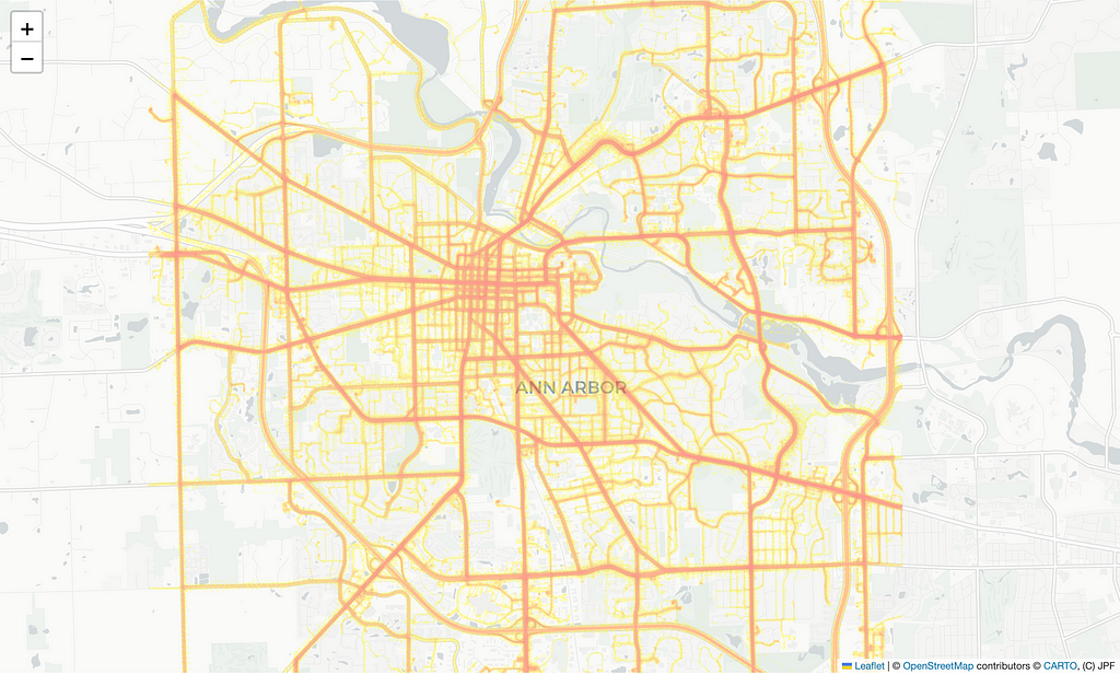
Next, you can open the map client and configure the density tile layer URI. Figure 8 below shows the Jupyter Notebook code cell to load the interactive map:
And that’s it! Figure 9 below displays the result.
My first foray into Rust was not nearly as difficult as I expected. I started by immersing myself in the available literature and YouTube videos before giving it a go. Next, I ensured I was using a helping hand with a great IDE from JetBrains: RustRover. Although still in preview mode, I found this IDE helpful and instructive when using Rust. Still, you will also be perfectly fine if you prefer Visual Studio Code. Just make sure you get the sanctioned plugins.
I used Grammarly to review the writing and accepted several of its rewriting suggestions.
JetBrains’ AI assistant wrote some of the code, and I also used it to learn Rust. It has become a staple of my everyday work with both Rust and Python.
The Extended Vehicle Energy Dataset is licensed under Apache 2.0, like its originator, the Vehicle Energy Dataset.
Vehicle Energy Dataset (GitHub)
João Paulo Figueira is a Data Scientist at tb.lx by Daimler Truck in Lisbon, Portugal.
Generating Map Tiles with Rust was originally published in Towards Data Science on Medium, where people are continuing the conversation by highlighting and responding to this story.
Originally appeared here:
Generating Map Tiles with Rust