Tag: AI

Reflections on How I Use AI in my University Lectures and Assessment

I would like to start with a clear disclaimer: While I have been lecturing at a university level since 2011, I am not a formally trained educator. What I am sharing in this article are my personal views and learning methods that I developed with my students. These might not necessarily be the same views as those of the University of Malta, where I lecture.

Generative AI requires educators to rethink assessment and embrace transparency for a student-centred, ethically informed learning future.

This is how I structured my reflections in this article:

• Why do I teach?
• How did we get here?
• Is AI a threat to Education?
• What can Educators do About It?
• What About Graded Work?
• Way Forward?

Why do I teach?

I am an AI scientist, and teaching is a core part of my academic role, which I enjoy. In class, I believe my duty is to find the most effective ways to communicate my research area to my students. My students are my peers, and we are on a learning journey together in an area of study that is fast-evolving and heavily impacting humanity. Since 2015, I have also been leading Malta’s Google Developers Group (GDG), allowing me to share learning experiences with different professionals.

In other words, my responsibility is two-fold: 1) Research the subject matter and 2) Facilitate my student’s learning experience by sharing my knowledge and pushing boundaries as a team.

How did we get here?

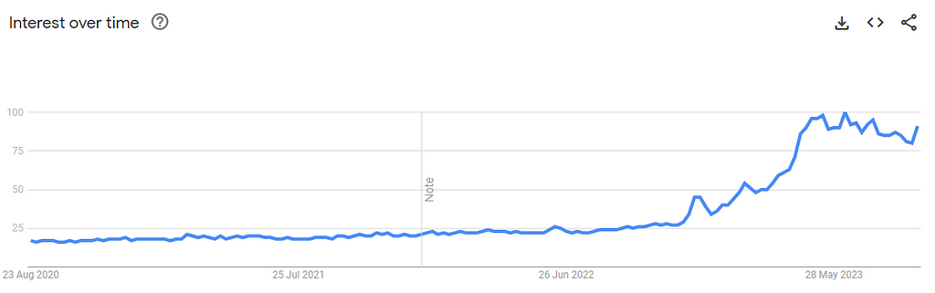
I was expecting the events of December 2022. At the end of May 2020, OpenAI released GPT3, demonstrating the capability of generating good-quality text with a few gentle prompts. It was the first time we could see an AI technique ‘writing something about itself,’ as this article reported. However, this was only accessible and ‘usable’ by those with a relatively strong technical background. In the summer of 2022, OpenAI released the beta version of its text-to-image generator DALL-E. Long story short: AI was getting better and more accessible month after month. I recently wrote another article about handling this fast rate of change.

ChatGPT, Gemini, Claude and all the generative AI products that followed made this transformative technology accessible.

Generative AI empowers us to explore countless topics and even achieve more. Do you need to draft an email complaint to your insurance company? Do you need to plan a marketing campaign? Do you need a SWOT analysis for your new project? Do you need a name for a pet? The list goes on. It’s there, quickly and freely accessible for anything we can think about.

So why not help us understand something better? Why not help students learn in more efficient and effective ways? Why not help us rethink our delivery?

Is AI a threat to education?

Short answer: No. Long answer: it’s a bit more complicated than it sounds.

EdTech or not?

This article is not about the formal aspect of EdTech or e-Learning. These terms generally refer to software and hardware or their combination with educational theory to facilitate learning. There is well-researched work, such as a book by Matthew Montebello, a colleague of mine, titled “AI-Injected e-Learning”, which covers this area more extensively. In this article, I focus on off-the-shelf chat interfaces I use in class.

Generative AI

The term ‘Generative AI’ does not help. While it fits most use cases, it triggers a negative connotation in education. [This is the same for art, which deserves another article.] As educators, we do not wish/want our students to generate answers for the tasks we give them and hand them in for grading. That is why there is usually an adverse first reaction to AI in the learning process.

But that’s only until we explore how this powerful technology can positively transform learning experiences—those of students and educators alike. From my experience, the more I use these methods in class, the more I broaden my expertise and knowledge in the subject area while finding better ways to communicate complex concepts.

Is it plagiarism?

I notice that many link the use of AI to plagiarism. The definition of plagiarism is “the unacknowledged use, as one’s own, of work of another person, whether or not such work has been published.” I do not wish to get into this debate, but I can comfortably say that I see a clear distinction between the use of AI and pre-AI plagiarism.

Shall we detect it using software?

Let’s be clear: It is wrong if a student or academic uses AI to generate content and submit it as if it were their work. It is academic misconduct, and it is helpful not to categorise it as plagiarism.

We expect authenticity when we consume any work, whether casual like this article or a formal academic paper. The lack of authenticity is what bothers us when it comes to plagiarism and using AI to generate content.

Generative AI works so well because (among other principles) it is based on a probabilistic approach. This means that every output differs from the one before, even if the same prompt is used to create it. If I copy someone else’s work and submit it as my own, what I copy is comparable and detected as plagiarism. Using Generative AI to create your work is a different form of misconduct. Because it is probabilistic, it follows detecting it is also probabilistic.

For this reason, I am against using any tool that claims to detect AI-generated content in an educational setting. While it can indicate whether someone used AI to generate work, the lack of certainty makes me uncomfortable taking action on a student, which might impact their career, when I know the possibility of the detection being a false positive.

If still in doubt, I wish to share that this is also OpenAI’s perspective. In January 2023 (less than a month after releasing ChatGPT), they launched an AI text classifier which claimed to predict whether a body of text is or is not AI-generated. Guess what happened? They shut it down by July 2023 because it was “impossible to make this prediction”. So why should you jeopardize a student’s future on an unreliable probabilistic decision?

What can educators do about it?

One of the main challenges in using AI is that it can limit critical thinking if students rely on generated answers. There is also a reasonable concern that this technology will deepen educational inequities if access to it is uneven.

Fight, Freeze or Flight? That would only mean we’re giving up on education because we have this new revolutionary technology. This is an opportunity and the start of a new era in education.

My three guiding principles in handling this are the following:

1. Transparency and Open Dialogue — We need these values in education, the workplace and society. So, let’s start by making it easy for our students to be transparent and open in how they use these tools in an educational setting where it should always be a safe space to try out new ideas.
2. Focus on the Learning Process—Education has (nearly) always been about the final output, be it examinations, assignments, or dissertations. This is an opportunity to shift the focus towards helping students demonstrate their thought processes in understanding the material and finding solutions to real-life problems.
3. Educate and Don’t Punish—We are there to educate and not punish, starting with a positive outlook. If we are transparent and provide students with a process that empowers them to be open about the way they use AI, we will have countless opportunities to give them constructive feedback about how they use this technology well without the need to punish them.

AI is providing me with an opportunity to renew the way I teach. This is how I am making the best out of this opportunity:

1. Personalised Learning — Ask students to prompt an AI system about a topic in various ways to help them better grasp the concept.
2. Stimulate Class Discussions—Invite students to discuss the output they got from AI systems and moderate the discussion to open the way for new topics to be explored while also handling any misconceptions about the topic.
3. Give students more realistic and real-life challenges — I use this to invite more mature students to apply topics covered in class to real-life scenarios or topics featured in current affairs.
4. Helping those with learning difficulties — If you know that some of your students have learning difficulties, AI can help you create variations of your content to tailor the variations to help students with different abilities.
5. Restructuring my courses — Once a course is over, I take feedback from students about what I can improve. I then combine the feedback with the course information and have ‘conversations’ with an AI system to help me reflect on fine-tuning the subsequent delivery, especially when introducing new topics.
6. Improving my course material — I find AI systems helpful when rewriting specific topics and pitching the delivery to students with varying backgrounds. You can also use Generative AI to suggest different ways of delivering the same content or material.

And what about graded work?

This is the elephant in the room. It’s easy to favour using AI to have a better experience in class, but what about its use during graded assignments or work?

I reflected a lot about this when this technology became very accessible. I decided to zoom out and look at the context holistically and from first principles. These are the principles upon which I base my decisions:

1. AI has been evolving for 80 years and is here to stay
2. These AI tools will only get better due to commercial interests in them
3. My students today are tomorrow’s workforce, and employers will expect them to use AI to be more productive
4. I want my students to be smart about using different tools and accountable to their leaders in how they use AI
5. There are so many topics which I wish to cover in class, but it is (till now) difficult to do so.

The way forward was/is clear: My duty is to design assessments that motivate my students, ensure their understanding, and prepare them to build a better tomorrow. The actionable way forward was to restructure my assessments to match this new reality and motivate students to use AI in an accountable manner.

Type of Assessment

The availability of AI challenged the nature of assessment. Some questions and tasks can be inputted as prompts, and students can get an outstanding output that they can submit without giving it much thought. While such behaviour is not right and shouldn’t happen, it also says a lot about the assessments we give students.

Consider the case of an essay about a concept, such as freedom of speech, where students would be expected to write 2000 words about the subject. The process would be that the students leave class and write the essay, submit it for correction, and the lecturer corrects it and gives a grade. This approach is an open invitation to the dilemmas I mentioned above.

Generative AI Journal

What do we look for in an employee? I believe that accountability tops the list because anything else follows. Based on this reasoning, I decided to develop the idea of a Generative AI Journal for my students to complete when they’re working on assignments I give. This journal explains how they used generative AI and how it went. In return, they get marks (in the region of 10%).

The key reasoning is the following. I am fine with my employees using AI to be more productive, but I need to know how they use it. This will help me be a better mentor and evaluate the task. Students are tomorrow’s employees. They will work in an environment where AI is available and ready for use. They will be expected to be as productive as possible. The aggregate of all these thoughts is that generative AI should be used accountable and transparently. Based on this reasoning, I came up with the idea of this journal. This 10-page journal is structured accordingly:

1. Introduction: Briefly describe the generative AI models (ChatGPT, Gemini, VS Co-Pilot, etc.) used and the rationale behind that choice. (Maximum of 1 page)
2. Ethical Considerations: Discuss the ethical aspects of using generative AI in the project. This should include issues like data bias and privacy together with measures of good academic conduct (Maximum of 1 page)
3. Methodology: Outline the methods and steps to integrate the generative AI model into the work. How did Generative AI fit into the assignment workflow?
4. Prompts and Responses: List the specific prompts used with the generative AI model that contributed to levelling up the work. Include the generated response for each prompt and explain how it improved your project.
5. Improvements and Contributions: Discuss the specific areas where generative AI enhanced the deliverables. This can include, but is not limited to, data analysis, formulation of ethical considerations, enhancement of literature reviews, or idea generation.
6. Individual Reflection: Reflection on the personal experience using generative AI in the project. Discuss what was learned, what surprised you, and how your perspective on using AI in academic projects has changed, if at all.
7. References and List of Resources Used

This is not something definitive. It is a work in progress that I am constantly updating to reflect the needs of my students and the context of the Generative AI evolution.

Way forward?

This is not a journey with a destination. The probable scenario is that education (and the workplace) will have to evolve along with the evolution of Generative AI.

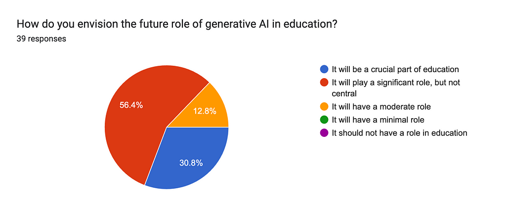
At the start of this article, I shared my perspective of seeing my students as my peers in the research journey. I’m linking this perspective to the way forward. At the end of the first semester of the academic year 2023/24, I distributed an anonymous questionnaire to 60 of my students. In this article, I am sharing the responses to two questions where I asked them what they thought about the way forward after using Generative AI, as described above.

When asked how they envision the future of Generative AI in education, 56% said that it will play a significant role but not central, with 12% saying it will only have a moderate role. 30% said that it will be a crucial part of education. This is meaningful because it shows that students feel and see the value in using this technology in class and that it should augment human educators rather than be a replacement.

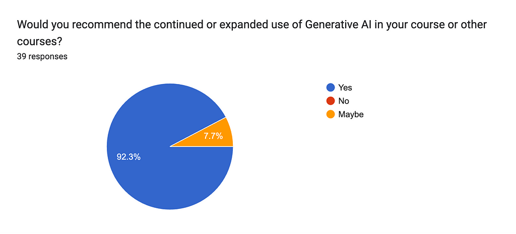
I asked my students for advice on whether I should keep using Generative AI in class. 92% think I should…and I will. The 8% were unsure, and that is also meaningful. Above all, this is a work in progress, and more work should be done to deliver meaningful educational experiences…but this doesn’t mean we shouldn’t start trying today.

This technology will improve every week and is here to stay. At the time of publishing this article, OpenAI released the GPT-4o Model and Google released countless AI products and features at the Google IO. We’re still scratching the surface of possibilities.

The future is not about fearing AI in the classroom. It is about using it as humanity’s latest invention to handle knowledge and information, hence empowering all stakeholders in the educational system.

Dr Dylan Seychell is a resident academic at the University of Malta’s Department of Artificial Intelligence, specialising in Computer Vision and Applied Machine Learning. With a background in academia and industry, he holds a PhD in Computer Vision and has published extensively on AI in international peer-reviewed conferences, journals and books.

Outside of the academic setting, he actively applies his expertise through his enterprise, focusing on enhancing tourist experiences through technological and cultural heritage innovations. He leads Malta’s Google Developers Group (GDG), is a technical expert certified by the Malta Digital Innovation Authority and is a Tourism Operators Business Section committee member within The Malta Chamber.

---

AI Knocking on the Classroom’s Door was originally published in Towards Data Science on Medium, where people are continuing the conversation by highlighting and responding to this story.

In this post, we present a new approach named multimodal RAG (mmRAG) to tackle those existing limitations in greater detail. The solution intends to address these limitations for practical generative artificial intelligence (AI) assistant use cases. Additionally, we examine potential solutions to enhance the capabilities of large language models (LLMs) and visual language models (VLMs) with advanced LangChain capabilities, enabling them to generate more comprehensive, coherent, and accurate outputs while effectively handling multimodal data

This post is co-written with Aurélien Capdecomme and Bertrand d’Aure from 20 Minutes. With 19 million monthly readers, 20 Minutes is a major player in the French media landscape. The media organization delivers useful, relevant, and accessible information to an audience that consists primarily of young and active urban readers. Every month, nearly 8.3 million 25–49-year-olds choose […]

Revolutionizing Large Dataset Feature Selection with Reinforcement Learning

Leverage the power of reinforcement learning for feature selection when faced with very large datasets

Discover how reinforcement learning transforms feature selection for machine learning models. Learn the process, implementation, and benefits of this innovative approach with practical examples and a dedicated Python library.

Feature selection is a determining step in the process of building a machine learning model. Selecting the good features for the model and the task that we want to achieve can definitely improve the performances. Indeed, a feature can add some noise and then disturb the model.

Also, selecting the features is especially more important if we are dealing with high-dimensional data set. It enables the model to learn faster and better. The idea is then to find the optimal number of features and the most meaningful ones.

In this article I will tackle this problem and go beyond by introducing a newly implemented method for feature selection. Although it exists many different feature selection processes they will not be introduced here since a lot of articles are already dealing with them. I will focus on the feature selection using the reinforcement learning strategy.

First, the reinforcement learning and more especially the Markov Decision Process will be addressed. It is a very new approach in the data science domain and more especially for feature selection purpose. After, I will introduce an implementation of this and how to install and use the python library (FSRLearning). Finally, I will prove the efficiency of this implementation. Among the possible feature selection approaches like wrappers or filtering, the reinforcement learning is the most powerful and efficient.

The goal of this article is to emphasise on the implementation for concret and real-problem oriented utilisation. The theoretical aspect of this problem will be simplified with examples although some references will be available at the end.

Reinforcement Learning : The Markov Decision Problem for feature selection

It has been demonstrated that reinforcement learning (RL) technics can be very efficient for problems like game solving. The concept of RL is based on Markovian Decision Process (MDP). The point here is not to define deeply the MDP but to get the general idea of how it works and how it can be useful to our problem.

The naive idea behind RL is that an agent starts in an unknown environnement. This agent has to take actions to complete a task. In function of the current state of the agent and the action he has selected previously, the agent will be more inclined to choose some actions. At every new state reached and action taken, the agent receives a reward. Here are then the main parameters that we need to define for feature selection purpose:

• What is a state ?
• What is an action ?
• What are the rewards ?
• How do we choose an action ?

Firstly, the state is merely a subset of features that exist in the data set. For example, if the data set has three features (Age, Gender, Height) plus one label, here will be the possible states:

[]                                              --> Empty set                           
[Age], [Gender], [Height]                       --> 1-feature set
[Age, Gender], [Gender, Height], [Age, Height]  --> 2-feature set
[Age, Gender, Height]                           --> All-feature set

In a state, the order of the features does not matter and it will be explained why a little bit later in the article. We have to consider it as a set and not a list of features.

Concerning the actions, from a subset we can go to any other subset with one not-already explored feature more than the current state. In the feature selection problem, an action is then selecting a not-already explored feature in the current state and add it to the next state. Here is a sample of possible actions:

[Age] -> [Age, Gender]
[Gender, Height] -> [Age, Gender, Height]

Here is an example of impossible actions:

[Age] -> [Age, Gender, Height]
[Age, Gender] -> [Age]
[Gender] -> [Gender, Gender]

We have defined the states and the actions but not the reward. The reward is a real number that is used for evaluating the quality of a state. For example if a robot is trying to reach the exit of a maze and decides to go to the exit as his next action, then the reward associated to this action will be “good”. If he selects as a next action to go in a trap then the reward will be “not good”. The reward is a value that brought information about the previous action taken.

In the problem of feature selection an interesting reward could be a value of accuracy that is added to the model by adding a new feature. Here is an example of how the reward is computed:

[Age] --> Accuracy = 0.65
[Age, Gender] --> Accuracy = 0.76
Reward(Gender) = 0.76 - 0.65 = 0.11

For each state that we visit for the first time a classifier will be trained with the set of features. This value is stored in the state and the training of the classifier, which is very costly, will only happens once even if the state is reached again later. The classifier does not consider the order of the feature. This is why we can see this problem as a graph and not a tree. In this example, the reward of the action of selecting Gender as a new feature for the model is the difference between the accuracy of the current state and the next state.

On the graph above, each feature has been mapped to a number (i.e “Age” is 1, “Gender” is 2 and “Height” is 3). It is totally possible to take other metrics to maximise to find the optimal set. In many business applications the recall is more considered than the accuracy.

The next important question is how do we select the next state from the current state or how do we explore our environement. We have to find the most optimal way to do it since it can quickly become a very complex problem. Indeed, if we naively explore all the possible set of features in a problem with 10 features, the number of states would be

10! + 2 = 3 628 802 possible states

The +2 is because we consider an empty state and a state that contains all the possible features. In this problem we would have to train the same model on all the states to get the set of features that maximises the accuracy. In the RL approach we will not have to go in all the states and to train a model every time that we go in an already visited state.

We had to determine some stop conditions for this problem and they will be detailed later. For now the epsilon-greedy state selection has been chosen. The idea is from a current state we select the next action randomly with a probability of epsilon (between 0 and 1 and often around 0.2) and otherwise select the action that maximises a function. For feature selection the function is the average of reward that each feature has brought to the accuracy of the model.

The epsilon-greedy algorithm implies two steps:

1. A random phase : with a probability epsilon, we select randomly the next state among the possible neighbours of the current state (we can imagine either a uniform or a softmax selection)
2. A greedy phase : we select the next state such that the feature added to the current state has the maximal contribution of accuracy to the model. To reduce the time complexity, we have initialised a list containing this values for each feature. This list is updated every time that a feature is chosen. The update is very optimal thanks to the following formula:

• AORf : Average of reward brought by the feature “f”
• k : number of times that “f” has been selected
• V(F) : state’s value of the set of features F (not detailed in this article for clarity reasons)

The global idea is to find which feature has brought the most accuracy to the model. That is why we need to browse different states to evaluate in many different environments the most global accurate value of a feature for the model.

Finally I will detail the two stop conditions. Since the goal is to minimise the number of state that the algorithm visits we need to be careful about them. The less never visited state we visit, the less amount of models we will have to train with different set of features. Training the model to get the accuracy is the most costly phase in terms of time and computation power.

1. The algorithm stops in any case in the final state which is the set containing all the features. We want to avoid reaching this state since it is the most expensive to train a model with.
2. Also, it stops browsing the graph if a sequence of visited states see their values degrade successively. A threshold has been set such that after square root of the number of total features in the dataset, it stops exploring.

Now that the modelling of the problem has been explained, we will detail the implementation in python.

The python library for Feature Selection with Reinforcement Learning

A python library resolving this problem is available. I will explain in this part how it works and prove that it is an efficient strategy. Also, this article stands as a documentation and you will be able to use this library for your projects by the end of the part.

1. The data pre-processing

Since we need to evaluate the accuracy of a state that is visited, we need to feed a model with the features and the data used for this feature selection task. The data has to been normalised, the categorical variables encoded and have as few rows as possible (the smallest it is, the fastest the algorithm will be). Also, it’s very important to create a mapping between the features and some integers as explained in the previous part. This step is not mandatory but very recommended. The final result of this step is to get a DataFrame with all the features and another with the labels to predict. Below is an example with a dataset used as a benchmark (it can be found here UCI Irvine Machine Learning Repository).

2. Installation and importation of the FSRLearning library

The second step is to install the library with pip. Here is the command to install it:

pip install FSRLearning

To import the library the following code can be used:

You will be able to create a feature selector simply by creating an object Feature_Selector_RL. Some parameters need to be filled in.

• feature_number (integer) : number of features in the DataFrame X
• feature_structure (dictionary) : dictionary for the graph implementation
• eps (float [0; 1]) : probability of choosing a random next state, 0 is an only greedy algorithm and 1 only random
• alpha (float [0; 1]): control the rate of updates, 0 is a very not updating state and 1 a very updated
• gamma (float [0, 1]): factor of moderation of the observation of the next state, 0 is a shortsighted condition and 1 it exhibits farsighted behavior
• nb_iter (int): number of sequences to go through the graph
• starting_state (“empty” or “random”) : if “empty”, the algorithm starts from the empty state and if “random”, the algorithm starts from a random state in the graph

All the parameters can be tuned but for most of the problem only few iterations can be good (around 100) and the epsilon value around 0.2 is often enough. The starting state is useful to browse the graph more efficiently but it can be very dependent on the dataset and both of the values can be tested.

Finally we can initialise very simply the selector with the following code:

Training the algorithm is very easy on the same basis than most of the ML library:

Here is an example of the output:

The output is a 5-tuple as follows:

• Index of the features in the DataFrame X (like a mapping)
• Number or times that the feature has been observed
• Average of reward brought by the feature after all the iterations
• Ranking of the features from the least to the most important (here 2 is the least and 7 the most important feature)
• Number of states globally visited

Another important method of this selector is to get a comparison with the RFE selector of Scikit-Learn. It takes as input X, y and the results of the selector.

The output is a print after each step of selection of the global metric of RFE and FSRLearning. It also outputs a visual comparison of the accuracy of the model with on the x-axis the number of features selected and on the y-axis the accuracy. The two horizontal lines are the median of accuracy for each method. Here is an example:

Average benchmark accuracy : 0.854251012145749, rl accuracy : 0.8674089068825909 
Median benchmark accuracy : 0.8552631578947368, rl accuracy : 0.868421052631579 
Probability to get a set of variable with a better metric than RFE : 1.0 
Area between the two curves : 0.17105263157894512

In this example the RL method has always given a better set of features for the model than RFE. We can then select with certainty among the sorted set of features any subset and it will give a better accuracy to the model. We can run several times the model and the comparator to get a very accurate estimation but the RL method is always better.

Another interesting method is the get_plot_ratio_exploration. It plots a graph comparing the number of already visited nodes and visited nodes in a sequence for a precise iteration.

Also, thanks to the second stop condition the time complexity of the algorithm decreases exponentially. Then even if the number of feature is big the convergence will be found quickly. The plot bellow is the number of times that a set of a certain size has been visited.

In all iterations the algorithm visited a state containing 6 variables or less. Beyond 6 variables we can see that the number of state reached is decreasing. It’s a good behaviour since it is faster to train a model with small set of features than the big ones.

Conclusion and references

Overall, we can see that the RL method is very efficient for maximising a metric of a model. It always converges quickly toward an interesting subset of features. Also, this method is very easy and fast to implement in ML projects with the FSRLearning library.

The github repository of the project with a complete documentation is available here.

If you wish to contact me, you can do so directly on linkedin here

This library has been implemented with the help of these two articles:

• Sali Rasoul, Sodiq Adewole and Alphonse Akakpo, FEATURE SELECTION USING REINFORCEMENT LEARNING (2021), ArXiv
• Seyed Mehdin Hazrati Fard, Ali Hamzeh and Sattar Hashemi, Using reinforcement learning to find an optimal set of features (2013), ScienceDirect

---

Reinforcement Learning for feature selection was originally published in Towards Data Science on Medium, where people are continuing the conversation by highlighting and responding to this story.

In this post, we explore a solution that addresses these challenges head-on using LoRA serving with Amazon SageMaker. By using the new performance optimizations of LoRA techniques in SageMaker large model inference (LMI) containers along with inference components, we demonstrate how organizations can efficiently manage and serve their growing portfolio of fine-tuned models, while optimizing costs and providing seamless performance for their customers. The latest SageMaker LMI container offers unmerged-LoRA inference, sped up with our LMI-Dist inference engine and OpenAI style chat schema. To learn more about LMI, refer to LMI Starting Guide, LMI handlers Inference API Schema, and Chat Completions API Schema.

Simple stream processing using Python and tumbling windows

In this tutorial, I want to show you how to downsample a stream of sensor data using only Python (and Redpanda as a message broker). The goal is to show you how simple stream processing can be, and that you don’t need a heavy-duty stream processing framework to get started.

Until recently, stream processing was a complex task that usually required some Java expertise. But gradually, the Python stream processing ecosystem has matured and there are a few more options available to Python developers — such as Faust, Bytewax and Quix. Later, I’ll provide a bit more background on why these libraries have emerged to compete with the existing Java-centric options.

But first let’s get to the task at hand. We will use a Python libary called Quix Streams as our stream processor. Quix Streams is very similar to Faust, but it has been optimized to be more concise in its syntax and uses a Pandas like API called StreamingDataframes.

You can install the Quix Streams library with the following command:

pip install quixstreams

What you’ll build

You’ll build a simple application that will calculate the rolling aggregations of temperature readings coming from various sensors. The temperature readings will come in at a relatively high frequency and this application will aggregate the readings and output them at a lower time resolution (every 10 seconds). You can think of this as a form of compression since we don’t want to work on data at an unnecessarily high resolution.

You can access the complete code in this GitHub repository.

This application includes code that generates synthetic sensor data, but in a real-world scenario this data could come from many kinds of sensors, such as sensors installed in a fleet of vehicles or a warehouse full of machines.

Here’s an illustration of the basic architecture:

Components of a stream processing pipeline

The previous diagram reflects the main components of a stream processing pipeline: You have the sensors which are the data producers, Redpanda as the streaming data platform, and Quix as the stream processor.

Data producers

These are bits of code that are attached to systems that generate data such as firmware on ECUs (Engine Control Units), monitoring modules for cloud platforms, or web servers that log user activity. They take that raw data and send it to the streaming data platform in a format that that platform can understand.

Streaming data platform

This is where you put your streaming data. It plays more or less the same role as a database does for static data. But instead of tables, you use topics. Otherwise, it has similar features to a static database. You’ll want to manage who can consume and produce data, what schemas the data should adhere to. Unlike a database though, the data is constantly in flux, so it’s not designed to be queried. You’d usually use a stream processor to transform the data and put it somewhere else for data scientists to explore or sink the raw data into a queryable system optimized for streaming data such as RisingWave or Apache Pinot. However, for automated systems that are triggered by patterns in streaming data (such as recommendation engines), this isn’t an ideal solution. In this case, you definitely want to use a dedicated stream processor.

Stream processors

These are engines that perform continuous operations on the data as it arrives. They could be compared to just regular old microservices that process data in any application back end, but there’s one big difference. For microservices, data arrives in drips like droplets of rain, and each “drip” is processed discreetly. Even if it “rains” heavily, it’s not too hard for the service to keep up with the “drops” without overflowing (think of a filtration system that filters out impurities in the water).

For a stream processor, the data arrives as a continuous, wide gush of water. A filtration system would be quickly overwhelmed unless you change the design. I.e. break the stream up and route smaller streams to a battery of filtration systems. That’s kind of how stream processors work. They’re designed to be horizontally scaled and work in parallel as a battery. And they never stop, they process the data continuously, outputting the filtered data to the streaming data platform, which acts as a kind of reservoir for streaming data. To make things more complicated, stream processors often need to keep track of data that was received previously, such as in the windowing example you’ll try out here.

Note that there are also “data consumers” and “data sinks” — systems that consume the processed data (such as front end applications and mobile apps) or store it for offline analysis (data warehouses like Snowflake or AWS Redshift). Since we won’t be covering those in this tutorial, I’ll skip over them for now.

Setting up a local streaming data cluster

In this tutorial, I’ll show you how to use a local installation of Redpanda for managing your streaming data. I’ve chosen Redpanda because it’s very easy to run locally.

You’ll use Docker compose to quickly spin up a cluster, including the Redpanda console, so make sure you have Docker installed first.

Creating the streaming applications

First, you’ll create separate files to produce and process your streaming data. This makes it easier to manage the running processes independently. I.e. you can stop the producer without stopping the stream processor too. Here’s an overview of the two files that you’ll create:

• The stream producer: sensor_stream_producer.py
  Generates synthetic temperature data and produces (i.e. writes) that data to a “raw data” source topic in Redpanda. Just like the Faust example, it produces the data at a resolution of approximately 20 readings every 5 seconds, or around 4 readings a second.
• The stream processor: sensor_stream_processor.py
  Consumes (reads) the raw temperature data from the “source” topic, performs a tumbling window calculation to decrease the resolution of the data. It calculates the average of the data received in 10-second windows so you get a reading for every 10 seconds. It then produces these aggregated readings to the agg-temperatures topic in Redpanda.

As you can see the stream processor does most of the heavy lifting and is the core of this tutorial. The stream producer is a stand-in for a proper data ingestion process. For example, in a production scenario, you might use something like this MQTT connector to get data from your sensors and produce it to a topic.

• For a tutorial, it’s simpler to simulate the data, so let’s get that set up first.

Creating the stream producer

You’ll start by creating a new file called sensor_stream_producer.py and define the main Quix application. (This example has been developed on Python 3.10, but different versions of Python 3 should work as well, as long as you are able to run pip install quixstreams.)

Create the file sensor_stream_producer.py and add all the required dependencies (including Quix Streams)

from dataclasses import dataclass, asdict # used to define the data schema
from datetime import datetime # used to manage timestamps
from time import sleep # used to slow down the data generator
import uuid # used for message id creation
import json # used for serializing data

from quixstreams import Application

Then, define a Quix application and destination topic to send the data.

app = Application(broker_address='localhost:19092')

destination_topic = app.topic(name='raw-temp-data', value_serializer="json")

The value_serializer parameter defines the format of the expected source data (to be serialized into bytes). In this case, you’ll be sending JSON.

Let’s use the dataclass module to define a very basic schema for the temperature data and add a function to serialize it to JSON.

@dataclass
class Temperature:
    ts: datetime
    value: int

    def to_json(self):
        # Convert the dataclass to a dictionary
        data = asdict(self)
        # Format the datetime object as a string
        data['ts'] = self.ts.isoformat()
        # Serialize the dictionary to a JSON string
        return json.dumps(data)

Next, add the code that will be responsible for sending the mock temperature sensor data into our Redpanda source topic.

i = 0
with app.get_producer() as producer:
    while i < 10000:
        sensor_id = random.choice(["Sensor1", "Sensor2", "Sensor3", "Sensor4", "Sensor5"])
       temperature = Temperature(datetime.now(), random.randint(0, 100))
        value = temperature.to_json()

        print(f"Producing value {value}")
        serialized = destination_topic.serialize(
            key=sensor_id, value=value, headers={"uuid": str(uuid.uuid4())}
        )
        producer.produce(
            topic=destination_topic.name,
            headers=serialized.headers,
            key=serialized.key,
            value=serialized.value,
        )
        i += 1
        sleep(random.randint(0, 1000) / 1000)

This generates 1000 records separated by random time intervals between 0 and 1 second. It also randomly selects a sensor name from a list of 5 options.

Now, try out the producer by running the following in the command line

python sensor_stream_producer.py

You should see data being logged to the console like this:

[data produced]

Once you’ve confirmed that it works, stop the process for now (you’ll run it alongside the stream processing process later).

Creating the stream processor

The stream processor performs three main tasks: 1) consume the raw temperature readings from the source topic, 2) continuously aggregate the data, and 3) produce the aggregated results to a sink topic.

Let’s add the code for each of these tasks. In your IDE, create a new file called sensor_stream_processor.py.

First, add the dependencies as before:

import os
import random
import json
from datetime import datetime, timedelta
from dataclasses import dataclass
import logging
from quixstreams import Application

logging.basicConfig(level=logging.INFO)
logger = logging.getLogger(__name__)

Let’s also set some variables that our stream processing application needs:

TOPIC = "raw-temperature" # defines the input topic
SINK = "agg-temperature"  # defines the output topic
WINDOW = 10  # defines the length of the time window in seconds
WINDOW_EXPIRES = 1 # defines, in seconds, how late data can arrive before it is excluded from the window

We’ll go into more detail on what the window variables mean a bit later, but for now, let’s crack on with defining the main Quix application.

app = Application(
    broker_address='localhost:19092',
    consumer_group="quix-stream-processor",
    auto_offset_reset="earliest",
)

Note that there are a few more application variables this time around, namely consumer_group and auto_offset_reset. To learn more about the interplay between these settings, check out the article “Understanding Kafka’s auto offset reset configuration: Use cases and pitfalls“

Next, define the input and output topics on either side of the core stream processing function and add a function to put the incoming data into a DataFrame.

input_topic = app.topic(TOPIC, value_deserializer="json")
output_topic = app.topic(SINK, value_serializer="json")

sdf = app.dataframe(input_topic)
sdf = sdf.update(lambda value: logger.info(f"Input value received: {value}"))

We’ve also added a logging line to make sure the incoming data is intact.

Next, let’s add a custom timestamp extractor to use the timestamp from the message payload instead of Kafka timestamp. For your aggregations, this basically means that you want to use the time that the reading was generated rather than the time that it was received by Redpanda. Or in even simpler terms “Use the sensor’s definition of time rather than Redpanda’s”.

def custom_ts_extractor(value):
 
    # Extract the sensor's timestamp and convert to a datetime object
    dt_obj = datetime.strptime(value["ts"], "%Y-%m-%dT%H:%M:%S.%f") # 

    # Convert to milliseconds since the Unix epoch for efficent procesing with Quix
    milliseconds = int(dt_obj.timestamp() * 1000)
    value["timestamp"] = milliseconds
    logger.info(f"Value of new timestamp is: {value['timestamp']}")

    return value["timestamp"]

# Override the previously defined input_topic variable so that it uses the custom timestamp extractor 
input_topic = app.topic(TOPIC, timestamp_extractor=custom_ts_extractor, value_deserializer="json") 

Why are we doing this? Well, we could get into a philosophical rabbit hole about which kind of time to use for processing, but that’s a subject for another article. With the custom timestamp, I just wanted to illustrate that there are many ways to interpret time in stream processing, and you don’t necessarily have to use the time of data arrival.

Next, initialize the state for the aggregation when a new window starts. It will prime the aggregation when the first record arrives in the window.

def initializer(value: dict) -> dict:

    value_dict = json.loads(value)
    return {
        'count': 1,
        'min': value_dict['value'],
        'max': value_dict['value'],
        'mean': value_dict['value'],
    }

This sets the initial values for the window. In the case of min, max, and mean, they are all identical because you’re just taking the first sensor reading as the starting point.

Now, let’s add the aggregation logic in the form of a “reducer” function.

def reducer(aggregated: dict, value: dict) -> dict:
    aggcount = aggregated['count'] + 1
    value_dict = json.loads(value)
    return {
        'count': aggcount,
        'min': min(aggregated['min'], value_dict['value']),
        'max': max(aggregated['max'], value_dict['value']),
        'mean': (aggregated['mean'] * aggregated['count'] + value_dict['value']) / (aggregated['count'] + 1)
    }

This function is only necessary when you’re performing multiple aggregations on a window. In our case, we’re creating count, min, max, and mean values for each window, so we need to define these in advance.

Next up, the juicy part — adding the tumbling window functionality:

### Define the window parameters such as type and length
sdf = (
    # Define a tumbling window of 10 seconds
    sdf.tumbling_window(timedelta(seconds=WINDOW), grace_ms=timedelta(seconds=WINDOW_EXPIRES))

    # Create a "reduce" aggregation with "reducer" and "initializer" functions
    .reduce(reducer=reducer, initializer=initializer)

    # Emit results only for closed 10 second windows
    .final()
)

### Apply the window to the Streaming DataFrame and define the data points to include in the output
sdf = sdf.apply(
    lambda value: {
        "time": value["end"], # Use the window end time as the timestamp for message sent to the 'agg-temperature' topic
        "temperature": value["value"], # Send a dictionary of {count, min, max, mean} values for the temperature parameter
    }
)

This defines the Streaming DataFrame as a set of aggregations based on a tumbling window — a set of aggregations performed on 10-second non-overlapping segments of time.

Tip: If you need a refresher on the different types of windowed calculations, check out this article: “A guide to windowing in stream processing”.

Finally, produce the results to the downstream output topic:

sdf = sdf.to_topic(output_topic)
sdf = sdf.update(lambda value: logger.info(f"Produced value: {value}"))

if __name__ == "__main__":
    logger.info("Starting application")
    app.run(sdf)

Note: You might wonder why the producer code looks very different to the producer code used to send the synthetic temperature data (the part that uses with app.get_producer() as producer()). This is because Quix uses a different producer function for transformation tasks (i.e. a task that sits between input and output topics).

As you might notice when following along, we iteratively change the Streaming DataFrame (the sdf variable) until it is the final form that we want to send downstream. Thus, the sdf.to_topic function simply streams the final state of the Streaming DataFrame back to the output topic, row-by-row.

The producer function on the other hand, is used to ingest data from an external source such as a CSV file, an MQTT broker, or in our case, a generator function.

Run the streaming applications

Finally, you get to run our streaming applications and see if all the moving parts work in harmony.

First, in a terminal window, start the producer again:

python sensor_stream_producer.py

Then, in a second terminal window, start the stream processor:

python sensor_stream_processor.py

Pay attention to the log output in each window, to make sure everything is running smoothly.

You can also check the Redpanda console to make sure that the aggregated data is being streamed to the sink topic correctly (you’ll fine the topic browser at: http://localhost:8080/topics).

Wrapping up

What you’ve tried out here is just one way to do stream processing. Naturally, there are heavy duty tools such Apache Flink and Apache Spark Streaming which are have also been covered extensively online. But — those are predominantly Java-based tools. Sure, you can use their Python wrappers, but when things go wrong, you’ll still be debugging Java errors rather than Python errors. And Java skills aren’t exactly ubiquitous among data folks who are increasingly working alongside software engineers to tune stream processing algorithms.

In this tutorial, we ran a simple aggregation as our stream processing algorithm, but in reality, these algorithms often employ machine learning models to transform that data — and the software ecosystem for machine learning is heavily dominated by Python.

An oft overlooked fact is that Python is the lingua franca for data specialists, ML engineers, and software engineers to work together. It’s even better than SQL because you can use it to do non-data-related things like make API calls and trigger webhooks. That’s one of the reasons why libraries like Faust, Bytewax and Quix evolved — to bridge the so-called impedance gap between these different disciplines.

Hopefully, I’ve managed to show you that Python is a viable language for stream processing, and that the Python ecosystem for stream processing is maturing at a steady rate and can hold its own against the older Java-based ecosystem.

• As a reminder, all the code for this tutorial is available in this GitHub repository.

---

Aggregating Real-time Sensor Data with Python and Redpanda was originally published in Towards Data Science on Medium, where people are continuing the conversation by highlighting and responding to this story.