Tag: AI

Implement the K-Means algorithm from scratch with this step-by-step Python tutorial

In this article, I show how I’d learn the K-Means algorithm if I’d started today. We’ll start with the fundamental concepts and implement a Python class that performs clustering tasks using nothing more than the Numpy package.

Whether you are a machine learning beginner trying to build a solid understanding of the concepts or a practitioner interested in creating custom machine learning applications and needs to understand how the algorithms work under the hood, that article is for you.

Table of contents

1. Introduction
2. What Does the K-Means algorithm do?
3. Implementation in Python
4. Evaluation and Interpretation
5. Conclusions and Next Steps

1. Introduction

Most of the machine learning algorithms widely used, such as Linear Regression, Logistic Regression, Decision Trees, and others are useful for making predictions from labeled data, that is, each input comprises feature values with a label value associated. That is what is called Supervised Learning.

However, often we have to deal with large sets of data with no label associated. Imagine a business that needs to understand the different groups of customers based on purchasing behavior, demographics, address, and other information, thus it can offer better services, products, and promotions.

These types of problems can be addressed with the use of Unsupervised Learning techniques. The K-Means algorithm is a widely used unsupervised learning algorithm in Machine Learning. Its simple and elegant approach makes it possible to separate a dataset into a desired number of K distinct clusters, thus allowing one to learn patterns from unlabelled data.

2. What Does the K-Means algorithm do?

As said earlier, the K-Means algorithm seeks to partition data points into a given number of clusters. The points within each cluster are similar, while points in different clusters have considerable differences.

Having said that, one question arises: how do we define similarity or difference? In K-Means clustering, the Euclidean distance is the most common metric for measuring similarity.

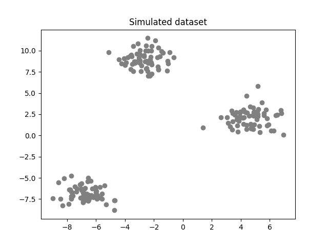
In the figure below, we can clearly see 3 different groups. Hence, we could determine the centers of each group and each point would be associated with the closest center.

By doing that, mathematically speaking, the idea is to minimize the within-cluster variance, the measurement of similarity between each point and its closest center.

Performing the task in the example above was straightforward because the data was two-dimensional and the groups were clearly distinct. However, as the number of dimensions increases and different values of K are considered, we need an algorithm to handle the complexity.

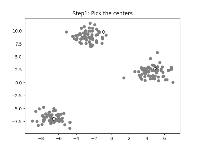
Step 1: Pick the initial centers (randomly)

We need to seed the algorithm with initial center vectors that can be chosen randomly from the data or generate random vectors with the same dimensions as the original data. See the white diamonds in the image below.

Step 2: Find the distances of each point to the centers

Now, we’ll calculate the distance of each data point to the K centers. Then we associate each point with the center closest to that point.

Given a dataset with N entries and M features, the distances to the centers c can be given by the following equation:

where:

k varies from 1 to K;

D is the distance of a point n to the k center;

x is the point vector;

c is the center vector.

Hence, for each data point n we’ll have K distances, then we have to label the vector to the center with the smallest distance:

Where D is a vector with K distances.

Step 3: Find the K centroids and iterate

For each of the K clusters, recalculate the centroid. The new centroid is the mean of all data points assigned to that cluster. Then update the positions of the centroids to the newly calculated.

Check if the centroids have changed significantly from the previous iteration. This can be done by comparing the positions of the centroids in the current iteration with those in the last iteration.

If the centroids have changed significantly, go back to Step 2. If not, the algorithm has converged and the process stops. See the image below.

3. Implementation in Python

Now that we know the fundamental concepts of the K-Means algorithm, it’s time to implement a Python class. The packages used were Numpy for mathematical calculations, Matplotlib for visualization, and the Make_blobs package from Sklearn for simulated data.

# import required packages
import numpy as np
import matplotlib.pyplot as plt
from sklearn.datasets import make_blobs

The class will have the following methods:

• Init method

A constructor method to initialize the basic parameters of the algorithm: the value k of clusters, the maximum number of iterations max_iter, and the tolerance tol value to interrupt the optimization when there is no significant improvement.

• Helper functions

These methods aim to assist the optimization process during training, such as calculating the Euclidean distance, randomly choosing the initial centroids, assigning the closest centroid to each point, updating the centroids’ values, and verifying whether the optimization converged.

• Fit and predict method

As mentioned earlier, the K-Means algorithm is an unsupervised learning technique, meaning it does not require labeled data during the training process. That way, it’s necessary a single method to fit the data and predict to which cluster each data point belongs.

• Total error method

A method to evaluate the quality of the optimization by calculating the total squared error of the optimization. That will be explored in the next section.

Here it goes the full code:

class Kmeans:
    
    # construct method for hyperparameter initialization
    def __init__(self, k=3, max_iter=100, tol=1e-06):
        self.k = k
        self.max_iter = max_iter
        self.tol = tol
  
    # randomly picks the initial centroids from the input data
    def pick_centers(self, X):
        centers_idxs = np.random.choice(self.n_samples, self.k)
        return X[centers_idxs]
    
    # finds the closest centroid for each data point
    def get_closest_centroid(self, x, centroids):
        distances = [euclidean_distance(x, centroid) for centroid in centroids]
        return np.argmin(distances)
    
    # creates a list with lists containing the idxs of each cluster
    def create_clusters(self, centroids, X):
        clusters = [[] for _ in range(self.k)]
        labels = np.empty(self.n_samples)
        for i, x in enumerate(X):
            centroid_idx = self.get_closest_centroid(x, centroids)
            clusters[centroid_idx].append(i)
            labels[i] = centroid_idx

        return clusters, labels
    
    # calculates the centroids for each cluster using the mean value 
    def compute_centroids(self, clusters, X):
        centroids = np.empty((self.k, self.n_features))
        for i, cluster in enumerate(clusters):
            centroids[i] = np.mean(X[cluster], axis=0)

        return centroids
    
    # helper function to verify if the centroids changed significantly
    def is_converged(self, old_centroids, new_centroids):
        distances = [euclidean_distance(old_centroids[i], new_centroids[i]) for i in range(self.k)]
        return (sum(distances) < self.tol)


    # method to train the data, find the optimized centroids and label each data point according to its cluster
    def fit_predict(self, X):
        self.n_samples, self.n_features = X.shape
        self.centroids = self.pick_centers(X)

        for i in range(self.max_iter):
            self.clusters, self.labels = self.create_clusters(self.centroids, X)
            new_centroids = self.compute_centroids(self.clusters, X)
            if self.is_converged(self.centroids, new_centroids):
                break
            self.centroids = new_centroids

    
    # method for evaluating the intracluster variance of the optimization
    def clustering_errors(self, X):
        cluster_values = [X[cluster] for cluster in self.clusters]
        squared_distances = []
        # calculation of total squared Euclidean distance
        for i, cluster_array in enumerate(cluster_values):
            squared_distances.append(np.sum((cluster_array - self.centroids[i])**2))

        total_error = np.sum(squared_distances)
        return total_error

4. Evaluation and Interpretation

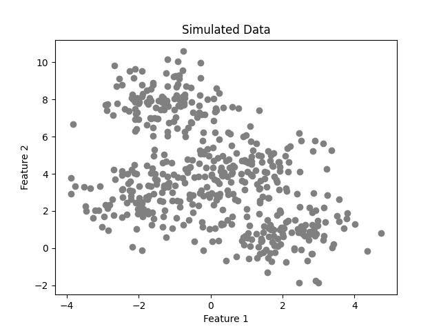
Now we’ll use the K-Means class to perform the clustering of simulated data. To do that, it’ll be used the make_blobs package from the Sklearn library. The data consists of 500 two-dimensional points with 4 fixed centers.

# create simulated data for examples
X, _ = make_blobs(n_samples=500, n_features=2, centers=4, 
                  shuffle=False, random_state=0)

After performing the training using four clusters, we achieve the following result.

model = Kmeans(k=4)
model.fit_predict(X)
labels = model.labels
centroids =model.centroids
plot_clusters(X, labels, centroids)

In that case, the algorithm was capable of calculating the clusters successfully with 18 iterations. However, we must keep in mind that we already know the optimal number of clusters from the simulated data. In real-world applications, we often don’t know that value.

As said earlier, the K-Means algorithm aims to make the within-cluster variance as small as possible. The metric used to calculate that variance is the total squared Euclidean distance given by:

where:

p is the number of data points in a cluster;

c_i is the centroid vector of a cluster;

K is the number of clusters.

In words, the formula above adds up the distances of the data points to the nearest centroid. The error decreases as the number K increases.

In the extreme case of K =N, you have one cluster for each data point and this error will be zero.

Willmott, Paul (2019).

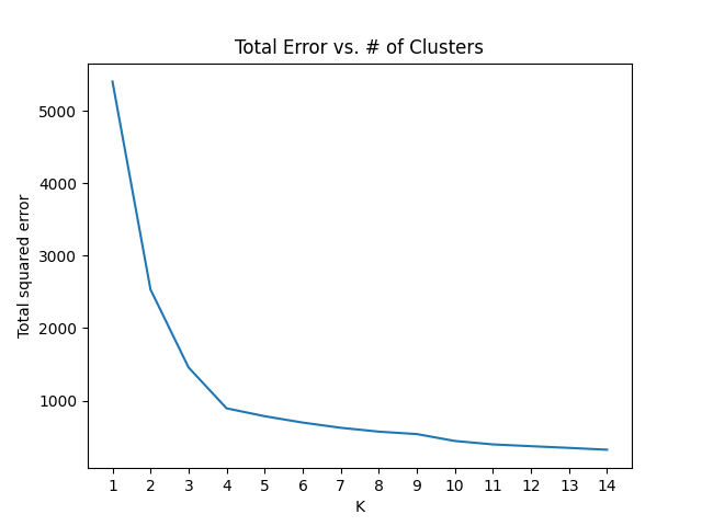
If we plot the error against the number of clusters and look at where the graph “bends”, we’ll be able to find the optimal number of clusters.

As we can see, the plot has an “elbow shape” and it bends at K = 4, meaning that for greater values of K, the decrease in the total error will be less significant.

5. Conclusions and Next Steps

In this article, we covered the fundamental concepts behind the K-Means algorithm, its uses, and applications. Also, using these concepts, we were able to implement a Python class from scratch that performed the clustering of simulated data and how to find the optimal value for K using a scree plot.

However, since we are dealing with an unsupervised technique, there is one additional step. The algorithm can successfully assign a label to the clusters, but the meaning of each label is a task that the data scientist or machine learning engineer will have to do by analyzing the data of each cluster.

In addition, I’ll leave some points for further exploration:

• Our simulated data used two-dimensional points. Try to use the algorithm for other datasets and find the optimal values for K.
• There are other unsupervised learning algorithms widely used such as Hierarchical Clustering.
• Depending on the domain of the problem, it may be necessary to use other error metrics such as Manhattan distance and cosine similarity. Try to investigate them.

Complete code available here:

ML-and-Ai-from-scratch/K-Means at main · Marcussena/ML-and-Ai-from-scratch

Please feel free to use and improve the code, comment, make suggestions, and connect with me on LinkedIn, X, and Github.

References

[1] Sebastian Raschka (2015), Python Machine Learning.

[2] Willmott, Paul. (2019). Machine Learning: An Applied Mathematics Introduction. Panda Ohana Publishing.

[3] Géron, A. (2017). Hands-On Machine Learning. O’Reilly Media Inc.

[4] Grus, Joel. (2015). Data Science from Scratch. O’Reilly Media Inc.

Mastering K-Means Clustering was originally published in Towards Data Science on Medium, where people are continuing the conversation by highlighting and responding to this story.

Get more out of your music data

Labeled audio data is chronically scarce in Music AI. In this post, I will share some tips on building strong models under these circumstances.

Compared to other fields like Computer Vision or Natural Language Processing (NLP), finding suitable public datasets for Music AI is often difficult. Whether you want to do mood recognition, noise detection, or instrument tagging: you will likely struggle to find the right data.

However, data scarcity affects not only hobby programmers and students. Aspiring music tech startups and even established music companies have the exact same problem. In the age of AI, many are desperately trying to gather proprietary data assets for machine learning purposes.

With that said, let us dive into my top 3 tips to get more out of your music data.

Tip 1: Apply Natural Data Augmentation

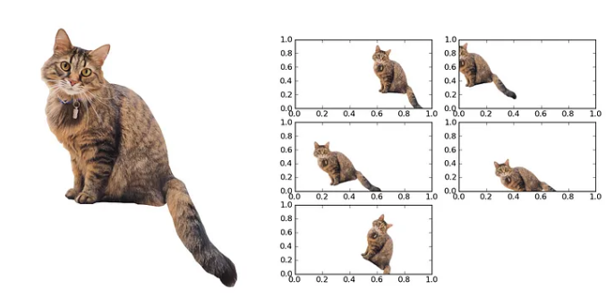
If you are a data scientist, you have probably heard about data augmentation. The basic idea is to take existing examples in our dataset and alter them slightly to produce new synthetic training examples. This is best illustrated with images. For instance, if our dataset contains an image of a cat, we can easily create new synthetic cats by shifting and rotating the original cat image.

Data augmentation is particularly effective for smaller datasets. If your dataset has only 100 images of cats, the odds that all possible angles and rotations are represented properly are low. These blind spots in the dataset will automatically translate to blind spots in the AI’s perception and judgment. By synthetically creating alterations of existing images, we can mitigate this risk.

Data Augmentation is Different in Music AI

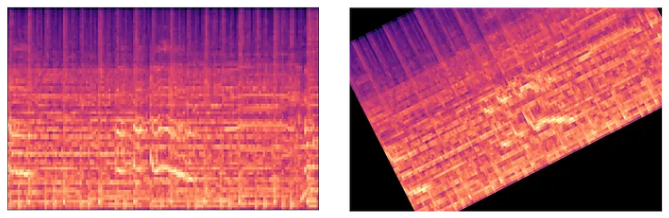
While data augmentation is a game-changer in Computer Vision, it is less straightforward in Music AI. The most common input to Music AI models is the spectrogram (learn more here). But have you tried rotating and shifting a spectrogram?

It is easy to see that the same tricks from Computer Vision cannot be applied directly to music AI. But why is this example so ridiculous? The answer is that, in contrast to the cat example, this kind of augmentation is not natural for a spectrogram.

An augmentation is natural when the changes made represent alterations that the model might encounter in real-world applications. While rotating a spectrogram certainly alters the data, visually, it is nonsensical and would never occur in practice. Instead, we need to find natural alterations specifically for music data.

Using Effects for Natural Audio Augmentation

The most common natural music data augmentation involves applying effects to the audio signal. There are a bunch of effects that every musician knows from their DAW:

• Time stretching
• Pitch shifting
• Compressors, Limiters, Distortion
• Reverb, Echo, Chorus
• and many more…

These effects can be applied to any piece of music, altering the data while preserving its main musical characteristics. If you want to know how to implement this in practice, check my article about this topic:

Natural Audio Data Augmentation Using Spotify’s Pedalboard

Data augmentation is not only used in many Music AI research papers, but I have also had great results with it myself. When data is scarce, data augmentation can push your model from unusable to acceptable. Even with higher data volumes, it adds that extra bit of reliability that can be crucial in production.

When implementing music data augmentation in practice, it is important to keep these three things in mind:

1. Stay natural. Listen to your data after augmentation and make sure it still sounds natural. Otherwise, your model might learn false patterns.
2. Not every training example should be augmented. To make sure that your model primarily learns from real, unaltered music, augmented examples should only be a portion of your training data (20–30%). You can also use sample weighting during training to adjust the impact of your augmented examples on the model.
3. Don’t augment your validation and test data. Augmentations help the model learn generalizable patterns. Your validation and test data should be unaltered to enable accurate benchmarks on real examples.

Time to boost your model effectiveness with data augmentation!

Tip 2: Use Smaller Models and Input Data

Bigger = Better?

In AI, bigger is often better — if there is enough data to feed these large models. However, with limited data, bigger models are more prone to overfitting. Overfitting occurs when the model memorizes patterns from the training data that do not generalize well to real-world data examples. But there is another way to approach this that I find even more compelling in this context.

Suppose you have a small dataset of spectrograms and are deciding between a small CNN model (100k parameters) or a large CNN (10 million parameters). Remember that every model parameter is effectively a best-guess number derived from the training dataset. If we think of it this way, it is obvious that it is easier for a model to get 100k parameters right than it is to nail 10 million.

In the end, both arguments lead to the same conclusion:

If data is scarce, consider building smaller models that focus only on the essential patterns.

But how can we achieve smaller models in practice?

Don’t Crack Walnuts with a Sledgehammer

My learning journey in Music AI has been dominated by deep learning. Up until a year ago, I had solved almost every problem using large neural networks. While this makes sense for complex tasks like music tagging or instrument recognition, not every task is that complicated.

For instance, a decent BPM estimator or key detector can be built without any machine learning by analyzing the time between onsets or by correlating chromagrams with key profiles, respectively.

Even for tasks like music tagging, it doesn’t always have to be a deep learning model. I’ve achieved good results in mood tagging through a simple K-Nearest Neighbor classifier over an embedding space (e.g. CLAP).

While most state-of-the-art methods in Music AI are based on deep learning, alternative solutions should be considered under data scarcity.

Pay Attention to the Data Input Size

More important than the choice of models is usually the choice of input data. In Music AI, we rarely use raw waveforms as input due to their data inefficiency. By transforming waveforms into (mel)spectrograms, we can decrease the input data dimensionality by a factor of 100 or more. This matters because large data inputs typically require larger and/or more complex models to process them.

To minimize the size of the model input, we can take two routes

1. Using smaller music snippets
2. Using more compressed/simplified music representations.

Using Smaller Music Snippets

Using smaller music snippets is especially effective if the outcome we are interested in is global, i.e. applies to every section of the song. For example, we can assume that the genre of a track remains relatively stable over the course of the track. Because of that, we can easily use 10-second snippets instead of full tracks (or the very common 30-second snippets) for a genre classification task.

This has two advantages:

1. Shorter snippets result in fewer data points per training example, allowing you to use smaller models.
2. By drawing three 10-second snippets instead of one 30-second snippet, we can triple the number of training observations. All in all, this means that we can build less data-hungry models and, at the same time, feed them more training examples than before.

However, there are two potential dangers here. Firstly, the snippet size must be long enough so that a classification is possible. For example, even humans struggle with genre classification when presented with 3-second snippets. We should choose the snippet size carefully and view this decision as a hyperparameter of our AI solution.

Secondly, not every musical attribute is global. For example, if a song features vocals, this doesn’t mean that there are no instrumental sections. If we cut the track into really short snippets, we would introduce many falsely-labelled examples into our training dataset.

Using More Efficient Music Representations

If you studied Music AI ten years ago (back when all of this was called “Music Information Retrieval”), you learned about chromagrams, MFCCs, and beat histograms. These handcrafted features were designed to make music data work with traditional ML approaches. With the rise of deep learning, it might seem like these features have been entirely replaced by (mel)spectrograms.

Spectrograms compress music into images without much information loss, making them ideal in combination with computer vision models. Instead of engineering custom features for different tasks, we can now use the same input data representation and model for most Music AI problems — provided you have tens of thousands of training examples to feed these models with.

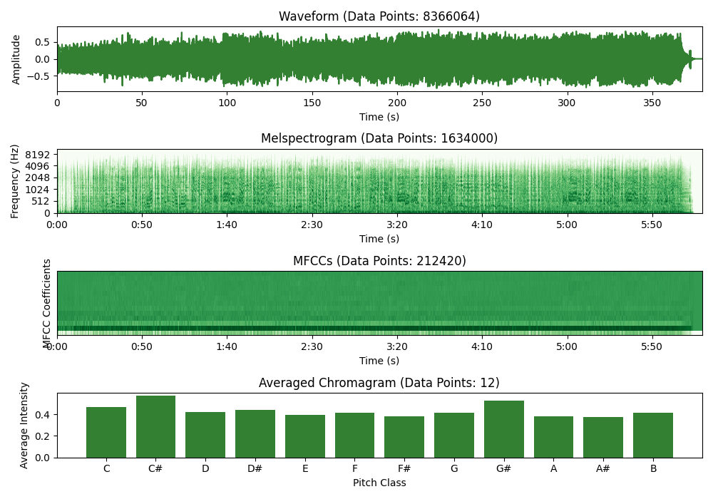
When data is scarce, we want to compress the information as much as possible to make it easier for the model to extract relevant patterns from the data. Consider these four music representations below and tell me which one helps you identify the musical key the fastest.

While mel spectrograms can be used as an input for key detection systems (and possibly should be if you have enough data), a simple chromagram averaged along the time dimension reveals this specific information much quicker. That is why spectrograms require complex models like CNNs while a chromagram can be easily analyzed by traditional models like logistic regression or decision trees.

In summary, the established spectrogram + CNN combination remains highly effective for many problems, provided you have enough data. However, with smaller datasets, it might make sense to revisit some feature engineering techniques from MIR or develop your own task-specific representations.

Tip 3: Leverage Pretrained Models or Embeddings

When data is scarce, one of the most effective strategies is to leverage pretrained models or embeddings. This approach allows you to build upon existing knowledge from models that have been trained on large datasets, thereby mitigating the limitations of your smaller dataset.

Why Use Pretrained Models?

Pretrained models have already learned to identify and extract meaningful features from their training data. For instance, a model trained on genre classification has likely learned a variety of meaningful musical patterns during training. If we now want to build our own mood tagging model, it might make sense to use the pretrained genre model as a starting point.

If the pretrained model was trained on a similar task, you can transfer their learned representations to your specific task. This process is known as transfer learning. Transfer learning can drastically reduce the amount of data and computational resources needed to train your own model from scratch.

Popular Pretrained Models in Music AI

A few years ago, the most common approach was to take pretrained models like genre classifiers and finetune them on specific tasks. Models like MusiCNN were commonly used for this.

However, nowadays, it is more common to use pretrained models that were specifically trained to yield meaningful music embeddings, i.e. vector representations of songs. Here are three pretrained embedding models that are commonly used:

1. Mert-v1 by m-a-p
2. CLAP by LAION
3. CLAP by Microsoft

From my personal experience, I’ve had the best results using Microsoft’s CLAP for transfer learning and LAION CLAP for similarity search.

Different Ways to Leverage Pretrained Models

Pretrained models can be used in a variety of ways:

1. Full Fine-Tuning: Use a pretrained classification or embedding model and fine-tune it on a smaller dataset of task-specific data. This method often achieves optimal results, if you can afford to use the full, large model for training and inference and know how to implement it.
2. Embeddings as Input Features: A more resource-efficient approach can be to extract embeddings from a pretrained model to use them as inputs for a new, much smaller model. As these embeddings are often 500–1000 dimensional vectors, a smaller neural network with a few thousand parameters can be attached to fine-tune more efficiently. For smaller datasets, this method is usually preferred over a full tine-tune.
3. Using Embeddings Directly: Even without any fine-tuning, embeddings can be used directly. For instance, embeddings from pretrained models are commonly used for music similarity search. CLAP models can even be used for text-to-music retrieval or (although still rather poorly) for zero-shot classification, i.e. classification without training.

Leveraging embeddings from pretrained models can significantly enhance your Music AI projects. By building on the learned pattern-recognition of these models, you avoid reinventing the wheel. When data is scarce, pretrained models should always be considered.

Conclusion

Don’t let data scarcity hold you back! Many use cases that required hundreds of thousands of training examples a few years ago have now essentially become commodities.

To achieve robust performance with small datasets, your number one priority should be not to waste any of your valuable data. Let’s review the main points from this article:

1. Data augmentation is a great way to let your models learn from training examples several times with small but effective variations, increasing robustness.
2. Smaller models and more efficient data representations force your model to focus on the most important, underlying patterns in the data, avoiding overfitting.
3. Pretrained models allow you to borrow some of the intelligence from larger AI systems through fine-tuning. No reason to train from scratch anymore!

Of course, there are natural limitations to what you can achieve with small datasets. If you have 100 labeled tracks and your goal is to build a multi-label genre classifier with 10 genres and 30 subgenres, you will not get very far — even if you use all of my tricks.

Still, I’ve developed surprisingly capable genre & mood classifiers with as little as 1000 labeled songs. Only 2 years ago, achieving this with such a small dataset would have been impossible. These democratization effects are one of the most exciting aspects of the current AI hype, in my opinion.

If you have a small but high-quality music dataset and are considering using it for machine learning, now is the best time to give it a try!

Interested in Music AI?

If you liked this article, you might want to check out some of my other work:

• “3 Music AI Breakthroughs to Expect in 2024”. Medium Blog
• “The Human Element in a World of Generative AI Music”. Video interview on the Audiosocket podcast
• “How Google Used Your Data to Improve their Music AI”. Medium Blog

You can also follow me on Linkedin to stay updated about new papers and trends in Music AI.

Thanks for reading this article!

3 Practical Tips to Combat Data Scarcity in Music AI was originally published in Towards Data Science on Medium, where people are continuing the conversation by highlighting and responding to this story.