Tag: AI

  • Interpretable Outlier Detection: Frequent Patterns Outlier Factor (FPOF)

    Interpretable Outlier Detection: Frequent Patterns Outlier Factor (FPOF)

    W Brett Kennedy

    An outlier detector method that supports categorical data and provides explanations for the outliers flagged

    Outlier detection is a common task in machine learning. Specifically, it’s a form of unsupervised machine learning: analyzing data where there are no labels. It’s the act of finding items in a dataset that are unusual relative to the others in the dataset.

    There can be many reasons to wish to identify outliers in data. If the data being examined is accounting records and we’re interested in finding errors or fraud, there are usually far too many transactions in the data to examine each manually, and it’s necessary to select a small, manageable number of transactions to investigate. A good starting point can be to find the most unusual records and examine these; this is with the idea the errors and fraud should both be rare enough to stand out as outliers.

    That is, not all outliers will be interesting, but errors and fraud will likely be outliers, so when looking for these, identifying the outliers can be a very practical technique.

    Or, the data may contain credit card transactions, sensor readings, weather measurements, biological data, or logs from websites. In all cases, it can be useful to identify the records suggesting errors or other problems, as well as the most interesting records.

    Often as well, outlier detection is used as part of business or scientific discovery, to better understand the data and the processes being described in the data. With scientific data, for example, we’re often interested in finding the most unusual records, as these may be the most scientifically interesting.

    The need for interpretability in outlier detection

    With classification and regression problems, it’s often preferable to use interpretable models. This can result in lower accuracy (with tabular data, the highest accuracy is usually found with boosted models, which are quite uninterpretable), but is also safer: we know how the models will handle unseen data. But, with classification and regression problems, it’s also common to not need to understand why individual predictions are made as they are. So long as the models are reasonably accurate, it may be sufficient to just let them make predictions.

    With outlier detection, though, the need for interpretability is much higher. Where an outlier detector predicts a record is very unusual, if it’s not clear why this may be the case, we may not know how to handle the item, or even if we should believe it is anomalous.

    In fact, in many situations, performing outlier detection can have limited value if there isn’t a good understanding of why the items flagged as outliers were flagged. If we are checking a dataset of credit card transactions and an outlier detection routine identifies a series of purchases that appear to be highly unusual, and therefore suspicious, we can only investigate these effectively if we know what is unusual about them. In some cases this may be obvious, or it may become clear after spending some time examining them, but it is much more effective and efficient if the nature of the anomalies is clear from when they are discovered.

    As with classification and regression, in cases where interpretability is not possible, it is often possible to try to understand the predictions using what are called post-hoc (after-the-fact) explanations. These use XAI (Explainable AI) techniques such as feature importances, proxy models, ALE plots, and so on. These are also very useful and will also be covered in future articles. But, there is also a very strong benefit to having results that are clear in the first place.

    In this article, we look specifically at tabular data, though will look at other modalities in later articles. There are a number of algorithms for outlier detection on tabular data commonly used today, including Isolation Forests, Local Outlier Factor (LOF), KNNs, One-Class SVMs, and quite a number of others. These often work very well, but unfortunately most do not provide explanations for the outliers found.

    Most outlier detection methods are straightforward to understand at an algorithm level, but it is nevertheless difficult to determine why some records were scored highly by a detector and others were not. If we process a dataset of financial transactions with, for example, an Isolation Forest, we can see which are the most unusual records, but may be at a loss as to why, especially if the table has many features, if the outliers contain rare combinations of multiple features, or the outliers are cases where no features are highly unusual, but multiple features are moderately unusual.

    Frequent Patterns Outlier Factor (FPOF)

    We’ve now gone over, at least quickly, outlier detection and interpretability. The remainder of this article is an excerpt from my book Outlier Detection in Python (https://www.manning.com/books/outlier-detection-in-python), which covers FPOF specifically.

    FPOF (FP-outlier: Frequent pattern based outlier detection) is one of a small handful of detectors that can provide some level of interpretability for outlier detection and deserves to be used in outlier detection more than it is.

    It also has the appealing property of being designed to work with categorical, as opposed to numeric, data. Most real-world tabular data is mixed, containing both numeric and categorical columns. But, most detectors assume all columns are numeric, requiring all categorical columns to be numerically encoded (using one-hot, ordinal, or another encoding).

    Where detectors, such as FPOF, assume the data is categorical, we have the opposite issue: all numeric features must be binned to be in a categorical format. Either is workable, but where the data is primarily categorical, it’s convenient to be able to use detectors such as FPOF.

    And, there’s a benefit when working with outlier detection to have at our disposal both some numeric detectors and some categorical detectors. As there are, unfortunately, relatively few categorical detectors, FPOF is also useful in this regard, even where interpretability is not necessary.

    The FPOF algorithm

    FPOF works by identifying what are called Frequent Item Sets (FISs) in a table. These are either values in a single feature that are very common, or sets of values spanning several columns that frequently appear together.

    Almost all tables contain a significant collection of FISs. FISs based on single values will occur so long as some values in a column are significantly more common than others, which is almost always the case. And FISs based on multiple columns will occur so long as there are associations between the columns: certain values (or ranges of numeric values) tend to be associated with other values (or, again, ranges of numeric values) in other columns.

    FPOF is based on the idea that, so long as a dataset has many frequent item sets (which almost all do), then most rows will contain multiple frequent item sets and inlier (normal) records will contain significantly more frequent item sets than outlier rows. We can take advantage of this to identify outliers as rows that contain much fewer, and much less frequent, FISs than most rows.

    Example with real-world data

    For a real-world example of using FPOF, we look at the SpeedDating set from OpenML (https://www.openml.org/search?type=data&sort=nr_of_likes&status=active&id=40536, licensed under CC BY 4.0 DEED).

    Executing FPOF begins with mining the dataset for the FISs. A number of libraries are available in Python to support this. For this example, we use mlxtend (https://rasbt.github.io/mlxtend/), a general-purpose library for machine learning. It provides several algorithms to identify frequent item sets; we use one here called apriori.

    We first collect the data from OpenML. Normally we would use all categorical and (binned) numeric features, but for simplicity here, we will just use only a small number of features.

    As indicated, FPOF does require binning the numeric features. Usually we’d simply use a small number (perhaps 5 to 20) equal-width bins for each numeric column. The pandas cut() method is convenient for this. This example is even a little simpler, as we just work with categorical columns.

    from mlxtend.frequent_patterns import apriori
    import pandas as pd
    from sklearn.datasets import fetch_openml
    import warnings

    warnings.filterwarnings(action='ignore', category=DeprecationWarning)

    data = fetch_openml('SpeedDating', version=1, parser='auto')
    data_df = pd.DataFrame(data.data, columns=data.feature_names)

    data_df = data_df[['d_pref_o_attractive', 'd_pref_o_sincere',
    'd_pref_o_intelligence', 'd_pref_o_funny',
    'd_pref_o_ambitious', 'd_pref_o_shared_interests']]
    data_df = pd.get_dummies(data_df)
    for col_name in data_df.columns:
    data_df[col_name] = data_df[col_name].map({0: False, 1: True})

    frequent_itemsets = apriori(data_df, min_support=0.3, use_colnames=True)

    data_df['FPOF_Score'] = 0

    for fis_idx in frequent_itemsets.index:
    fis = frequent_itemsets.loc[fis_idx, 'itemsets']
    support = frequent_itemsets.loc[fis_idx, 'support']
    col_list = (list(fis))
    cond = True
    for col_name in col_list:
    cond = cond & (data_df[col_name])

    data_df.loc[data_df[cond].index, 'FPOF_Score'] += support

    min_score = data_df['FPOF_Score'].min()
    max_score = data_df['FPOF_Score'].max()
    data_df['FPOF_Score'] = [(max_score - x) / (max_score - min_score)
    for x in data_df['FPOF_Score']]

    The apriori algorithm requires all features to be one-hot encoded. For this, we use panda’s get_dummies() method.

    We then call the apriori method to determine the frequent item sets. Doing this, we need to specify the minimum support, which is the minimum fraction of rows in which the FIS appears. We don’t want this to be too high, or the records, even the strong inliers, will contain few FISs, making them hard to distinguish from outliers. And we don’t want this too low, or the FISs may not be meaningful, and outliers may contain as many FISs as inliers. With a low minimum support, apriori may also generate a very large number of FISs, making execution slower and interpretability lower. In this example, we use 0.3.

    It’s also possible, and sometimes done, to set restrictions on the size of the FISs, requiring they relate to between some minimum and maximum number of columns, which may help narrow in on the form of outliers you’re most interested in.

    The frequent item sets are then returned in a pandas dataframe with columns for the support and the list of column values (in the form of the one-hot encoded columns, which indicate both the original column and value).

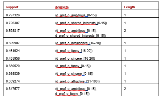
    To interpret the results, we can first view the frequent_itemsets, shown next. To include the length of each FIS we add:

    frequent_itemsets['length'] = 
    frequent_itemsets['itemsets'].apply(lambda x: len(x))

    There are 24 FISs found, the longest covering three features. The following table shows the first ten rows, sorting by support.

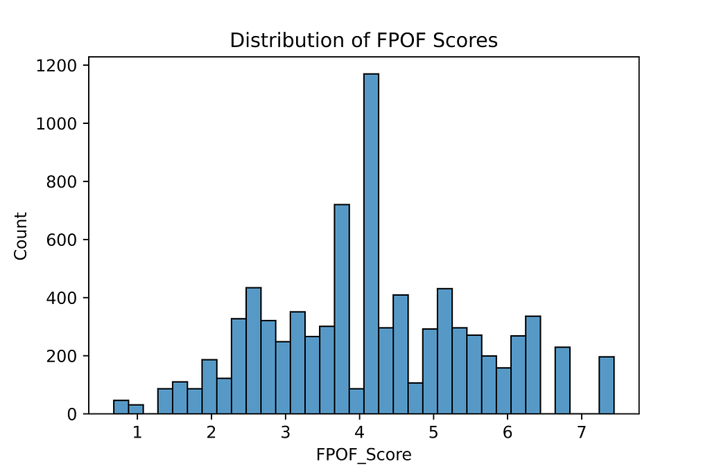
    We then loop through each frequent item set and increment the score for each row that contains the frequent item set by the support. This can optionally be adjusted to favor frequent item sets of greater lengths (with the idea that a FIS with a support of, say 0.4 and covering 5 columns is, everything else equal, more relevant than an FIS with support of 0.4 covering, say, 2 columns), but for here we simply use the number and support of the FISs in each row.

    This actually produces a score for normality and not outlierness, so when we normalize the scores to be between 0.0 and 1.0, we reverse the order. The rows with the highest scores are now the strongest outliers: the rows with the least and the least common frequent item sets.

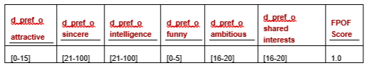
    Adding the score column to the original dataframe and sorting by the score, we see the most normal row:

    We can see the values for this row match the FISs well. The value for d_pref_o_attractive is [21–100], which is an FIS (with support 0.36); the values for d_pref_o_ambitious and d_pref_o_shared_interests are [0–15] and [0–15], which is also an FIS (support 0.59). The other values also tend to match FISs.

    The most unusual row is shown next. This matches none of the identified FISs.

    As the frequent item sets themselves are quite intelligible, this method has the advantage of producing reasonably interpretable results, though this is less true where many frequent item sets are used.

    The interpretability can be reduced, as outliers are identified not by containing FISs, but by not, which means explaining a row’s score amounts to listing all the FISs it does not contain. However, it is not strictly necessary to list all missing FISs to explain each outlier; listing a small set of the most common FISs that are missing will be sufficient to explain outliers to a decent level for most purposes. Statistics about the the FISs that are present and the the normal numbers and frequencies of the FISs present in rows provides good context to compare.

    One variation on this method uses the infrequent, as opposed to frequent, item sets, scoring each row by the number and rarity of each infrequent itemset they contain. This can produce useful results as well, but is significantly more computationally expensive, as many more item sets need to be mined, and each row is tested against many FISs. The final scores can be more interpretable, though, as they are based on the item sets found, not missing, in each row.

    Conclusions

    Other than the code here, I am not aware of an implementation of FPOF in python, though there are some in R. The bulk of the work with FPOF is in mining the FISs and there are numerous python tools for this, including the mlxtend library used here. The remaining code for FPOP, as seen above, is fairly simple.

    Given the importance of interpretability in outlier detection, FPOF can very often be worth trying.

    In future articles, we’ll go over some other interpretable methods for outlier detection as well.

    All images are by author


    Interpretable Outlier Detection: Frequent Patterns Outlier Factor (FPOF) was originally published in Towards Data Science on Medium, where people are continuing the conversation by highlighting and responding to this story.

    Originally appeared here:
    Interpretable Outlier Detection: Frequent Patterns Outlier Factor (FPOF)

    Go Here to Read this Fast! Interpretable Outlier Detection: Frequent Patterns Outlier Factor (FPOF)

  • Profiling CUDA using Nsight Systems: A Numba Example

    Carlos Costa, Ph.D.

    Profiling CUDA Using Nsight Systems: A Numba Example

    Learn about profiling by inspecting concurrent and parallel Numba CUDA code in Nsight Systems

    Introduction

    Optimization is a crucial part of writing high performance code, no matter if you are writing a web server or computational fluid dynamics simulation software. Profiling allows you to make informed decisions regarding your code. In a sense, optimization without profiling is like flying blind: mostly fine for seasoned professionals with expert knowledge and fine-tuned intuition, but a recipe for disaster for almost everyone else.

    Photo by Rafa Sanfilippo on Unsplash

    In This Tutorial

    Following my initial series CUDA by Numba Examples (see parts 1, 2, 3, and 4), we will study a comparison between unoptimized, single-stream code and a slightly better version which uses stream concurrency and other optimizations. We will learn, from the ground-up, how to use NVIDIA Nsight Systems to profile and analyze CUDA code. All the code in this tutorial can also be found in the repo cako/profiling-cuda-nsight-systems.

    Nsight Systems

    NVIDIA recommends as best practice to follow the APOD framework (Assess, Parallelize, Optimize, Deploy). There are a variety of proprietary, open-source, free, and commercial software for different types of assessments and profiling. Veteran Python users may be familiar with basic profilers such as cProfile, line_profiler, memory_profiler (unfortunately, unmaintaned as of 2024) and more advanced tools like PyInstrument and Memray. These profilers target specific aspects of the “host” such as CPU and RAM usage.

    However, profiling “device” (e.g., GPU) code — and its interactions with the host — requires specialized tools provided by the device vendor. For NVIDIA GPUs, Nsight Systems, Nsight Compute, Nsight Graphics are available for profiling different aspects of computation. In this tutorial we will focus on using Nsight Systems, which is a system-wide profiler. We will use it to profile Python code which interacts with the GPU via Numba CUDA.

    To get started, you will need Nsight Systems CLI and GUI. The CLI can be installed separately and will be used to profile the code in a GPGPU-capable system. The full version includes both CLI and GUI. Note that both versions could be installed in a system without a GPU. Grab the version(s) you need from the NVIDIA website.

    To make it easier to visualize code sections in the GUI, NVIDIA also provides the Python pip and conda-installable library nvtx which we will use to annotate sections of our code. More on this later.

    Setting Everything Up: A Simple Example

    In this section we will set our development and profiling environment up. Below are two very simple Python scripts: kernels.py and run_v1.py. The former will contain all CUDA kernels, and the latter will serve as the entry point to run the example. In this example we are following the “reduce” pattern introduced in article CUDA by Numba Examples Part 3: Streams and Events to compute the sum of an array.

    #%%writefile kernels.py
    import numba
    from numba import cuda

    THREADS_PER_BLOCK = 256
    BLOCKS_PER_GRID = 32 * 40


    @cuda.jit
    def partial_reduce(array, partial_reduction):
    i_start = cuda.grid(1)
    threads_per_grid = cuda.blockDim.x * cuda.gridDim.x
    s_thread = numba.float32(0.0)
    for i_arr in range(i_start, array.size, threads_per_grid):
    s_thread += array[i_arr]

    s_block = cuda.shared.array((THREADS_PER_BLOCK,), numba.float32)
    tid = cuda.threadIdx.x
    s_block[tid] = s_thread
    cuda.syncthreads()

    i = cuda.blockDim.x // 2
    while i > 0:
    if tid < i:
    s_block[tid] += s_block[tid + i]
    cuda.syncthreads()
    i //= 2

    if tid == 0:
    partial_reduction[cuda.blockIdx.x] = s_block[0]


    @cuda.jit
    def single_thread_sum(partial_reduction, sum):
    sum[0] = numba.float32(0.0)
    for element in partial_reduction:
    sum[0] += element


    @cuda.jit
    def divide_by(array, val_array):
    i_start = cuda.grid(1)
    threads_per_grid = cuda.gridsize(1)
    for i in range(i_start, array.size, threads_per_grid):
    array[i] /= val_array[0]
    #%%writefile run_v1.py
    import argparse
    import warnings

    import numpy as np
    from numba import cuda
    from numba.core.errors import NumbaPerformanceWarning

    from kernels import (
    BLOCKS_PER_GRID,
    THREADS_PER_BLOCK,
    divide_by,
    partial_reduce,
    single_thread_sum,
    )

    # Ignore NumbaPerformanceWarning
    warnings.simplefilter("ignore", category=NumbaPerformanceWarning)


    def run(size):
    # Define host array
    a = np.ones(size, dtype=np.float32)
    print(f"Old sum: {a.sum():.3f}")

    # Array copy to device and array creation on the device.
    dev_a = cuda.to_device(a)
    dev_a_reduce = cuda.device_array((BLOCKS_PER_GRID,), dtype=dev_a.dtype)
    dev_a_sum = cuda.device_array((1,), dtype=dev_a.dtype)

    # Launching kernels to normalize array
    partial_reduce[BLOCKS_PER_GRID, THREADS_PER_BLOCK](dev_a, dev_a_reduce)
    single_thread_sum[1, 1](dev_a_reduce, dev_a_sum)
    divide_by[BLOCKS_PER_GRID, THREADS_PER_BLOCK](dev_a, dev_a_sum)

    # Array copy to host
    dev_a.copy_to_host(a)
    cuda.synchronize()
    print(f"New sum: {a.sum():.3f}")


    def main():
    parser = argparse.ArgumentParser(description="Simple Example v1")
    parser.add_argument(
    "-n",
    "--array-size",
    type=int,
    default=100_000_000,
    metavar="N",
    help="Array size",
    )

    args = parser.parse_args()
    run(size=args.array_size)


    if __name__ == "__main__":
    main()

    This is a simple script that can just be run with:

    $ python run_v1.py
    Old sum: 100000000.000
    New sum: 1.000

    We also run this code through our profiler, which just entails calling nsys with some options before the call to our script:

    $ nsys profile 
    --trace cuda,osrt,nvtx
    --gpu-metrics-device=all
    --cuda-memory-usage true
    --force-overwrite true
    --output profile_run_v1
    python run_v1.py
    GPU 0: General Metrics for NVIDIA TU10x (any frequency)
    Old sum: 100000000.000
    New sum: 1.000
    Generating '/tmp/nsys-report-fb78.qdstrm'
    [1/1] [========================100%] profile_run_v1.nsys-rep
    Generated:
    /content/profile_run_v1.nsys-rep

    You can consult the Nsight CLI docs for all the available options to the nsys CLI. For this tutorial we will always use the ones above. Let’s dissect this command:

    • profile puts nsys in profile mode. There are many other modes like export and launch.
    • –trace cuda,osrt,nvtx ensures we “listen” to all CUDA calls (cuda), OS runtime library calls (osrt) and nvtx annotations (none in this example). There are many more trace options such as cublas, cudnn, mpi,dx11 and several others. Check the docs for all options.
    • –gpu-metrics-device=all records GPU metrics for all GPUs, including Tensor Core usage.
    • –cuda-memory-usage tracks GPU memory usage of kernels. It may significantly slow down execution and requires –trace=cuda. We use it because our scripts our pretty fast anyways.

    Navigating the Nsight Systems GUI

    If the command exited successfully, we will have a profile_run_v1.nsys-rep in the current folder. We will open this file by launching the Nsight Systems GUI, File > Open. The initial view is slightly confusing. So we will start by decluttering: resize the Events View port to the bottom, and minimize CPU, GPU and Processes under the Timeline View port. Now expand only Processes > python > CUDA HW. See Figures 1a and 1b.

    Figure 1a: Opening an nsys report and decluttering the interface. Credits: Own work. CC BY-SA 4.0.
    Figure 1b: nsys report showing host-to-device memory operations (green), device-to-host memory operations (red) and CUDA kernels (blue). Credits: Own work. CC BY-SA 4.0.

    First up, let’s find our kernels. On the CUDA HW line, you will find green and red blobs, and very small slivers of light blue (see Figure 1b). If you hover over those you will see tooltips saying, “CUDA Memory operations in progress” for red and green, and “CUDA Kernel Running (89.7%)” for the light blues. These are going to be the bread and butter of our profiling. On this line, we will be able to tell when and how memory is being transferred (red and green) and when and how our kernels are running (light blue).

    Let’s dig in a little bit more on our kernels. You should see three very small blue slivers, each representing a kernel call. We will zoom into the region by clicking and dragging the mouse from just before the start of the first kernel call to just after the end of the last one, and then pressing Shift + Z. See Figure 2.

    Figure 2: Navigating an nsys report and zooming into an area of interest. Credits: Own work. CC BY-SA 4.0.

    Now that we have found our kernels, let’s see some metrics. We open the GPU > GPU Metrics tabs for that. In this panel, can find “Warp Occupancy” (beige) for compute kernels. One way to optimize CUDA code is to ensure that the warp occupancy is as close to 100% as possible for as long as possible. This means that our GPU is not idling. We notice that this is happening for the first and last kernels but not the middle kernel. That is expected as the middle kernel launches a single thread. One final thing to note in this section is the GPU > GPU Metrics > SMs Active > Tensor Active / FP16 Active line. This line will show whether the tensor cores are being used. In this case you should verify that they are not.

    Now let’s briefly look at the Events View. Right click Processes > python > CUDA HW and click “Show in Events View”. Then sort the events by descending duration. In Figure 3, we see that the slowest events are two pageable memory transfers. We have seen in CUDA by Numba Examples Part 3: Streams and Events that pageable memory transfers can be suboptimal, and we should prefer page-locked or “pinned” memory transfers. If we have slow memory transfers due to use of pageable memory, the Events View can be a great location to identify where these slow transfers can be found. Pro tip: you can isolate memory transfers by right clicking Processes > python > CUDA HW > XX% Memory instead.

    Figure 3. Events View in Nsight Systems showing a pageable (non-pinned) memory transfer. Credits: Own work. CC BY-SA 4.0.

    In this section we learned how to profile a Python program which uses CUDA, and how to visualize basic information of this program in the Nsight Systems GUI. We also noticed that in this simple program, we are using pageable instead of pinned memory, that one of our kernels is not occupying all warps, that the GPU is idle for quite some time between kernels being run and that we are not using tensor cores.

    Annotating with NVTX

    In this section we will learn how to improve our profiling experience by annotation sections in Nsight Systems with NVTX. NVTX allows us to mark different regions of the code. It can mark ranges and instantaneous events. For a deeper look, check the docs. Below we create run_v2.py, which, in addition to annotating run_v1.py, also changes this line:

    a = np.ones(size, dtype=np.float32)

    to these:

    a = cuda.pinned_array(size, dtype=np.float32)
    a[...] = 1.0

    Therefore, in addition to the annotations, we are now using a pinned memory. If you want to learn more about the different types of memories that CUDA supports, see the CUDA C++ Programming Guide. It is of relevance that this is not the only way to pin an array in Numba. A previously created Numpy array can also be created with a context, as explained in the Numba documentation.

    #%%writefile run_v2.py
    import argparse
    import warnings

    import numpy as np
    import nvtx
    from numba import cuda
    from numba.core.errors import NumbaPerformanceWarning

    from kernels import (
    BLOCKS_PER_GRID,
    THREADS_PER_BLOCK,
    divide_by,
    partial_reduce,
    single_thread_sum,
    )

    # Ignore NumbaPerformanceWarning
    warnings.simplefilter("ignore", category=NumbaPerformanceWarning)


    def run(size):
    with nvtx.annotate("Compilation", color="red"):
    dev_a = cuda.device_array((BLOCKS_PER_GRID,), dtype=np.float32)
    dev_a_reduce = cuda.device_array((BLOCKS_PER_GRID,), dtype=dev_a.dtype)
    dev_a_sum = cuda.device_array((1,), dtype=dev_a.dtype)
    partial_reduce[BLOCKS_PER_GRID, THREADS_PER_BLOCK](dev_a, dev_a_reduce)
    single_thread_sum[1, 1](dev_a_reduce, dev_a_sum)
    divide_by[BLOCKS_PER_GRID, THREADS_PER_BLOCK](dev_a, dev_a_sum)

    # Define host array
    a = cuda.pinned_array(size, dtype=np.float32)
    a[...] = 1.0
    print(f"Old sum: {a.sum():.3f}")

    # Array copy to device and array creation on the device.
    with nvtx.annotate("H2D Memory", color="yellow"):
    dev_a = cuda.to_device(a)
    dev_a_reduce = cuda.device_array((BLOCKS_PER_GRID,), dtype=dev_a.dtype)
    dev_a_sum = cuda.device_array((1,), dtype=dev_a.dtype)

    # Launching kernels to normalize array
    with nvtx.annotate("Kernels", color="green"):
    partial_reduce[BLOCKS_PER_GRID, THREADS_PER_BLOCK](dev_a, dev_a_reduce)
    single_thread_sum[1, 1](dev_a_reduce, dev_a_sum)
    divide_by[BLOCKS_PER_GRID, THREADS_PER_BLOCK](dev_a, dev_a_sum)

    # Array copy to host
    with nvtx.annotate("D2H Memory", color="orange"):
    dev_a.copy_to_host(a)
    cuda.synchronize()
    print(f"New sum: {a.sum():.3f}")


    def main():
    parser = argparse.ArgumentParser(description="Simple Example v2")
    parser.add_argument(
    "-n",
    "--array-size",
    type=int,
    default=100_000_000,
    metavar="N",
    help="Array size",
    )

    args = parser.parse_args()
    run(size=args.array_size)


    if __name__ == "__main__":
    main()

    Comparing the two files, you can see it’s as simple as wrapping some GPU kernel calls with

    with nvtx.annotate("Region Title", color="red"):
    ...

    Pro tip: you can also annotate functions by placing the @nvtx.annotate decorator above their definition, automatically annotate everything by calling your script with python -m nvtx run_v2.py, or apply the autoannotator selectively in you code by enabling or disabling nvtx.Profile(). See the docs!

    Let’s run this new script and open the results in Nsight Systems.

    $ nsys profile 
    --trace cuda,osrt,nvtx
    --gpu-metrics-device=all
    --cuda-memory-usage true
    --force-overwrite true
    --output profile_run_v2
    python run_v2.py
    GPU 0: General Metrics for NVIDIA TU10x (any frequency)
    Old sum: 100000000.000
    New sum: 1.000
    Generating '/tmp/nsys-report-69ab.qdstrm'
    [1/1] [========================100%] profile_run_v2.nsys-rep
    Generated:
    /content/profile_run_v2.nsys-rep

    Again, we start by minimizing everything, leaving only Processes > python > CUDA HW open. See Figure 4. Notice that we now have a new line, NVTX. On this line in the timeline window we should see different colored blocks corresponding to the annotation regions that we created in the code. These are Compilation, H2D Memory, Kernels and D2H Memory. Some of these my be too small to read, but will be legible if you zoom into the region.

    Figure 4. Example of NVTX annotations and an Events View with pinned memory. Credits: Own work. CC BY-SA 4.0.

    The profiler confirms that this memory is pinned, ensuring that our code is truly using pinned memory. In addition, H2D Memory and D2H Memory are now taking less than half of the time that they were taking before. Generally we can expect better performance using pinned memory or prefetched mapped arrays (not supported by Numba).

    Stream Concurrency

    Now we will investigate whether we can improve this code by introducing streams. The idea is that while memory transfers are occurring, the GPU can start processing the data. This allows a level of concurrency, which hopefully will ensure that we are occupying our warps as fully as possible.

    Figure 5. Using different streams may allow for concurrent execution. Credits: Zhang et al. 2021 (CC BY 4.0).

    In the code below we will split the processing of our array into roughly equal parts. Each part will run in a separate stream, including transferring data and computing the sum of the array. Then, we synchronize all streams and sum their partial sums. At this point we can then launch normalization kernels for each stream independently.

    We want to answer a few questions:

    1. Will the code below truly create concurrency? Could we be introducing a bug?
    2. Is it faster than the code which uses a single stream?
    3. Is the warp occupancy better?
    #%%writefile run_v3_bug.py
    import argparse
    import warnings
    from math import ceil

    import numpy as np
    import nvtx
    from numba import cuda
    from numba.core.errors import NumbaPerformanceWarning

    from kernels import (
    BLOCKS_PER_GRID,
    THREADS_PER_BLOCK,
    divide_by,
    partial_reduce,
    single_thread_sum,
    )

    # Ignore NumbaPerformanceWarning
    warnings.simplefilter("ignore", category=NumbaPerformanceWarning)


    def run(size, nstreams):
    with nvtx.annotate("Compilation", color="red"):
    dev_a = cuda.device_array((BLOCKS_PER_GRID,), dtype=np.float32)
    dev_a_reduce = cuda.device_array((BLOCKS_PER_GRID,), dtype=dev_a.dtype)
    dev_a_sum = cuda.device_array((1,), dtype=dev_a.dtype)
    partial_reduce[BLOCKS_PER_GRID, THREADS_PER_BLOCK](dev_a, dev_a_reduce)
    single_thread_sum[1, 1](dev_a_reduce, dev_a_sum)
    divide_by[BLOCKS_PER_GRID, THREADS_PER_BLOCK](dev_a, dev_a_sum)

    # Define host array
    a = cuda.pinned_array(size, dtype=np.float32)
    a[...] = 1.0

    # Define regions for streams
    step = ceil(size / nstreams)
    starts = [i * step for i in range(nstreams)]
    ends = [min(s + step, size) for s in starts]
    print(f"Old sum: {a.sum():.3f}")

    # Create streams
    streams = [cuda.stream()] * nstreams

    cpu_sums = [cuda.pinned_array(1, dtype=np.float32) for _ in range(nstreams)]
    devs_a = []
    with cuda.defer_cleanup():
    for i, (stream, start, end) in enumerate(zip(streams, starts, ends)):
    cpu_sums[i][...] = np.nan

    # Array copy to device and array creation on the device.
    with nvtx.annotate(f"H2D Memory Stream {i}", color="yellow"):
    dev_a = cuda.to_device(a[start:end], stream=stream)
    dev_a_reduce = cuda.device_array(
    (BLOCKS_PER_GRID,), dtype=dev_a.dtype, stream=stream
    )
    dev_a_sum = cuda.device_array((1,), dtype=dev_a.dtype, stream=stream)
    devs_a.append(dev_a)

    # Launching kernels to sum array
    with nvtx.annotate(f"Sum Kernels Stream {i}", color="green"):
    for _ in range(50): # Make it spend more time in compute
    partial_reduce[BLOCKS_PER_GRID, THREADS_PER_BLOCK, stream](
    dev_a, dev_a_reduce
    )
    single_thread_sum[1, 1, stream](dev_a_reduce, dev_a_sum)
    with nvtx.annotate(f"D2H Memory Stream {i}", color="orange"):
    dev_a_sum.copy_to_host(cpu_sums[i], stream=stream)

    # Ensure all streams are caught up
    cuda.synchronize()

    # Aggregate all 1D arrays into a single 1D array
    a_sum_all = sum(cpu_sums)

    # Send it to the GPU
    with cuda.pinned(a_sum_all):
    with nvtx.annotate("D2H Memory Default Stream", color="orange"):
    dev_a_sum_all = cuda.to_device(a_sum_all)

    # Normalize via streams
    for i, (stream, start, end, dev_a) in enumerate(
    zip(streams, starts, ends, devs_a)
    ):
    with nvtx.annotate(f"Divide Kernel Stream {i}", color="green"):
    divide_by[BLOCKS_PER_GRID, THREADS_PER_BLOCK, stream](
    dev_a, dev_a_sum_all
    )

    # Array copy to host
    with nvtx.annotate(f"D2H Memory Stream {i}", color="orange"):
    dev_a.copy_to_host(a[start:end], stream=stream)

    cuda.synchronize()
    print(f"New sum: {a.sum():.3f}")


    def main():
    parser = argparse.ArgumentParser(description="Simple Example v3")
    parser.add_argument(
    "-n",
    "--array-size",
    type=int,
    default=100_000_000,
    metavar="N",
    help="Array size",
    )
    parser.add_argument(
    "-s",
    "--streams",
    type=int,
    default=4,
    metavar="N",
    help="Array size",
    )

    args = parser.parse_args()
    run(size=args.array_size, nstreams=args.streams)


    if __name__ == "__main__":
    main()

    Let’s run the code and collect results.

    $ nsys profile 
    --trace cuda,osrt,nvtx
    --gpu-metrics-device=all
    --cuda-memory-usage true
    --force-overwrite true
    --output profile_run_v3_bug_4streams
    python run_v3_bug.py -s 4
    GPU 0: General Metrics for NVIDIA TU10x (any frequency)
    Old sum: 100000000.000
    New sum: 1.000
    Generating '/tmp/nsys-report-a666.qdstrm'
    [1/1] [========================100%] profile_run_v3_bug_4streams.nsys-rep
    Generated:
    /content/profile_run_v3_bug_4streams.nsys-rep

    The program ran and yielded the correct answer. But when we open the profiling file (see Figure 6), we notice that there are two streams instead of 4! And one is basically completely idle! What’s going on here?

    Figure 6. Example of buggy multi-stream code. Credits: Own work. CC BY-SA 4.0.

    There is a bug in the creation of the streams. By doing

    streams = [cuda.stream()] * nstreams

    we are actually creating a single stream and repeating it nstreams times. So why are we seeing two streams instead of one? The fact that one is not doing much computation should be an indicator that there is a stream that we are not using. This stream is the default stream, which we are not using at all in out code since all GPU interactions are given a stream, the stream we created.

    We can fix this bug with:

    streams = [cuda.stream() for _ in range(nstreams)]
    # Ensure they are all different
    assert all(s1.handle != s2.handle for s1, s2 in zip(streams[:-1], streams[1:]))

    The code above will also ensure they are really different streams, so it would have caught the bug had we had it in the code. It does so by checking the stream pointer value.

    Now we can run the fixed code with 1 stream and 8 streams for comparison. See Figures 7 and 8, respectively.

    $  nsys profile 
    --trace cuda,osrt,nvtx
    --gpu-metrics-device=all
    --cuda-memory-usage true
    --force-overwrite true
    --output profile_run_v3_1stream
    python run_v3.py -s 1
    GPU 0: General Metrics for NVIDIA TU10x (any frequency)
    Old sum: 100000000.000
    New sum: 1.000
    Generating '/tmp/nsys-report-de65.qdstrm'
    [1/1] [========================100%] profile_run_v3_1stream.nsys-rep
    Generated:
    /content/profile_run_v3_1stream.nsys-rep
    $ nsys profile 
    --trace cuda,osrt,nvtx
    --gpu-metrics-device=all
    --cuda-memory-usage true
    --force-overwrite true
    --output profile_run_v3_8streams
    python run_v3.py -s 8
    GPU 0: General Metrics for NVIDIA TU10x (any frequency)
    Old sum: 100000000.000
    New sum: 1.000
    Generating '/tmp/nsys-report-1fb7.qdstrm'
    [1/1] [========================100%] profile_run_v3_8streams.nsys-rep
    Generated:
    /content/profile_run_v3_8streams.nsys-rep
    Figure 7. Example of single stream code. Credits: Own work. CC BY-SA 4.0.
    Figure 7. Example of correct multi-stream code. Credits: Own work. CC BY-SA 4.0.

    Again, both give correct results. By opening the one with 8 streams we see that yes, the bug has been fixed (Figure 7). Indeed, we now see 9 streams (8 created + default). In addition, we see that they are working at the same time! So we have achieved concurrency!

    Unfortunately, if we dig a bit deeper we notice that the concurrent code is not necessarily faster. On my machine the critical section of both versions, from start of memory transfer to the last GPU-CPU copy takes around 160 ms.

    A likely culprit is the warp occupancy. We notice that the warp occupancy is significantly better in the single-stream version. The gains we are getting in this example in compute are likely being lost by not occupying our GPU as efficiently. This is likely related to the structure of the code which (artificially) calls way too many kernels. In addition, if all threads are filled by a single stream, there is no gain in concurrency, since other streams have to be idle until resources free up.

    This example is important because it shows that our preconceived notions of performance are just hypotheses. They need to be verified.

    At this point of APOD, we have assessed, parallelized (both through threads and concurrency) and so the next step would be to deploy. We also noticed a slight performance regression with concurrency, so for this example, a single-stream version would likely be the one deployed. In production, the next step would be to follow the next piece of code which is best suited for parallelization and restarting APOD.

    Conclusion

    In this article we saw how to set up, use and interpret results from profiling Python code in NVIDIA Nsight Systems. C and C++ code can be analyzed very similarly, and indeed most of the material out there uses C and C++ examples.

    We also show how profiling can allow us to catch bugs and performance test our programs, ensuring that the features we introduce truly are improving performance, and if they are not, why.


    Profiling CUDA using Nsight Systems: A Numba Example was originally published in Towards Data Science on Medium, where people are continuing the conversation by highlighting and responding to this story.

    Originally appeared here:
    Profiling CUDA using Nsight Systems: A Numba Example

    Go Here to Read this Fast! Profiling CUDA using Nsight Systems: A Numba Example

  • From Assumptions to Accuracy: The Role of Conditional Probability in Real-World Predictions

    Atisha Rajpurohit

    Conditional probability is better than probability ; IF you have the relevant information

    Image taken from Unsplash

    Introduction

    Anyone who has ever studied probability has heard of the long-established definition of probability of “Probability can be defined as the number of favorable outcomes divided by the total number outcomes.” I can still hear my 4th grade teacher reiterating this!

    While this definition is correct, it often makes me wonder, how accurate is this definition for the real-world? How accurate is it when we have some more information about the favorable outcomes? To put it more clearly, when we have some more “conditions” to put to our favorable outcomes.

    Putting “conditions” is like slicing your original pie of number of favorable outcomes in a number of ways, using multiple conditions, to give you the slice that represents the number of favorable outcomes for you more truly. The image below attempts to depict this concept in a very brief manner.

    Image created by Author

    What better way than to represent what is in the mind’s of a lot of international data science students studying in the US and looking for jobs! The original number of available jobs is depicted on the extreme left.

    1st Condition : Introducing the 1st condition for “Work Experience Duration” refines the slice for the number of available jobs for a new joiner.

    2nd Condition : Furthermore, introducing the 2nd condition for “Nationality/Citizenship” refines the slice even more.

    3rd Condition : The small dark blue slice in the extreme right chart represents the most accurate representation for the number of available jobs (number of favorable outcomes).

    Before proceeding into why conditional probability may be better than probability, let’s do a quick recap of the definitions.

    2. Definition of probability and conditional probability

    Probability :

    P(A) = Number of favorable outcomes for A / Total number of outcomes

    Conditional probability :

    Now consider two events A and B. The foundation of conditional probability is when there is an “event given another event”. In this case, when one says A given B, what that means is the event A occurring given event B has occurred. So that is attaching the “condition of B, to A”.

    P(A|B) = P(A intersection B) / P(B) where

    P(A intersection B)* is given as the probability of both event A and event B occurring.

    *given (A intersection B) and (A’ intersection B) are mutually exclusive. Hence (A intersection B) union (A’ intersection B) = B.

    After defining these slightly confusing definitions, I will move to why I think conditional probability is actually better.

    3. Example — Inspiration for this article

    To start off, the reason I got an idea for this article was when I was watching a Bollywood movie the other day and when there was a scene about two old friends discussing the probability of them bumping into each other!

    Let me introduce some more information about this scene:

    • 1st friend : Police officer, originally from Mumbai city, who was traveling to Kalimpong; a small town, for a case.
    • 2nd friend : Math professor, who was a resident of the town — Kalimpong.

    These friends know each other since they both studied in the same university.

    • Currently, the friends met each other at a cafe where the professor would go everyday.

    After introducing this information, let’s go back to what was the probability of both of them bumping into each other in Kalimpong.

    Police Officer : “Bro, what are the chances!”

    Math Professor : “One out of 95675”

    Police Officer : “Wrong! You did not count me”

    Math Professor “I did. The current population is 95674”

    Hmm… so let’s break this logic :

    Initial Probability Calculation:

    • The math professor calculated the probability of meeting his friend, the police officer as 1/95,675.
    • This assumes that all the 95,674 residents of Kalimpong have the same probability of meeting the professor as the police officer.

    Why is this calculation inaccurate:

    • This calculation assumes that meeting the police officer is the same as meeting ANY OTHER resident of Kalimpong!

    Introducing conditional probability:

    Let’s consider some specific scenarios

    I. Relevant Information:

    • The police officer is a resident of Mumbai who traveled to Kalimpong.
    • The math professor goes to this cafe every day.
    • The police officer happened to go to the same cafe this one time.

    II. Conditional Events:

    Event A: The professor and police officer meet in Kalimpong.

    Event B: The police officer travels from Mumbai to Kalimpong .

    Probability of the two friends meeting :

    1. The probability of police officer traveling from Mumbai to Kalimpong, depends on factors such as:

    • How often does he travel for work?
    • How often does he get assigned to cases from small towns?
    • Let’s assume this probability is 0.1%.

    2. The probability of the two friends meeting, depends on factors such as:

    • How often do they both go to the cafe?
    • How popular is the cafe?
    • The professor regularly goes to the cafe.
    • Let’s assume this probability is 1%.

    Final calculations :

    • The probability of the two friends meeting in Kalimpong, given that the police officer is there, is 0.001%.
    • This is a simplistic representation of the concept, but what I am trying to say is to always look for more relevant information to refine your probability.

    Conclusion

    Probability is simple and complicated at the same time! However there is always refining we can do with any additional information that we are provided. In real world situations, always try to look for how additional information can help you add conditions to make your probabilities more accurate.

    Thank you for reading and I hope this article was useful to you!


    From Assumptions to Accuracy: The Role of Conditional Probability in Real-World Predictions was originally published in Towards Data Science on Medium, where people are continuing the conversation by highlighting and responding to this story.

    Originally appeared here:
    From Assumptions to Accuracy: The Role of Conditional Probability in Real-World Predictions

    Go Here to Read this Fast! From Assumptions to Accuracy: The Role of Conditional Probability in Real-World Predictions

  • Accelerate Mixtral 8x7B pre-training with expert parallelism on Amazon SageMaker

    Accelerate Mixtral 8x7B pre-training with expert parallelism on Amazon SageMaker

    Roy Allela

    Mixture of Experts (MoE) architectures for large language models (LLMs) have recently gained popularity due to their ability to increase model capacity and computational efficiency compared to fully dense models. By utilizing sparse expert subnetworks that process different subsets of tokens, MoE models can effectively increase the number of parameters while requiring less computation per […]

    Originally appeared here:
    Accelerate Mixtral 8x7B pre-training with expert parallelism on Amazon SageMaker

    Go Here to Read this Fast! Accelerate Mixtral 8x7B pre-training with expert parallelism on Amazon SageMaker

  • Generating fashion product descriptions by fine-tuning a vision-language model with SageMaker and Amazon Bedrock

    Generating fashion product descriptions by fine-tuning a vision-language model with SageMaker and Amazon Bedrock

    Antonia Wiebeler

    This post shows you how to predict domain-specific product attributes from product images by fine-tuning a VLM on a fashion dataset using Amazon SageMaker, and then using Amazon Bedrock to generate product descriptions using the predicted attributes as input. So you can follow along, we’re sharing the code in a GitHub repository.

    Originally appeared here:
    Generating fashion product descriptions by fine-tuning a vision-language model with SageMaker and Amazon Bedrock

    Go Here to Read this Fast! Generating fashion product descriptions by fine-tuning a vision-language model with SageMaker and Amazon Bedrock