
Originally appeared here:
Evaluating ChatGPT in Data Science: Churn Prediction Analysis As An Example

The paper “Attention is All You Need” debuted perhaps the single largest advancement in Natural Language Processing (NLP) in the last 10 years: the Transformer [1]. This architecture massively simplified the complex designs of language models at the time while achieving unparalleled results. State-of-the-art (SOTA) models, such as those in the GPT, Claude, and Llama families, owe their success to this design, at the heart of which is self-attention. In this deep dive, we will explore how this mechanism works and how it is used by transformers to create contextually rich embeddings that enable these models to perform so well.
1 — Overview of the Transformer Embedding Process
3 — The Self-Attention Mechanism
4 — Transformer Embeddings in Python
5 — Conclusion
6 — Further Reading
In the prelude article of this series, we briefly explored the history of the Transformer and its impact on NLP. To recap: the Transformer is a deep neural network architecture that is the foundation for almost all LLMs today. Derivative models are often called Transformer-based models or transformers for short, and so these terms will be used interchangeably here. Like all machine learning models, transformers work with numbers and linear algebra rather than processing human language directly. Because of this, they must convert textual inputs from users into numerical representations through several steps. Perhaps the most important of these steps is applying the self-attention mechanism, which is the focus of this article. The process of representing text with vectors is called embedding (or encoding), hence the numerical representations of the input text are known as transformer embeddings.
In Part 2 of this series, we explored static embeddings for language models using word2vec as an example. This embedding method predates transformers and suffers from one major drawback: the lack of contextual information. Words with multiple meanings (called polysemous words) are encoded with somewhat ambiguous representations since they lack the context needed for precise meaning. A classic example of a polysemous word is bank. Using a static embedding model, the word bank would be represented in vector space with some degree of similarity to words such as money and deposit and some degree of similarity to words such as river and nature. This is because the word will occur in many different contexts within the training data. This is the core problem with static embeddings: they do not change based on context — hence the term “static”.
Transformers overcome the limitations of static embeddings by producing their own context-aware transformer embeddings. In this approach, fixed word embeddings are augmented with positional information (where the words occur in the input text) and contextual information (how the words are used). These two steps take place in distinct components in transformers, namely the positional encoder and the self-attention blocks, respectively. We will look at each of these in detail in the following sections. By incorporating this additional information, transformers can produce much more powerful vector representations of words based on their usage in the input sequence. Extending the vector representations beyond static embeddings is what enables Transformer-based models to handle polysemous words and gain a deeper understanding of language compared to previous models.
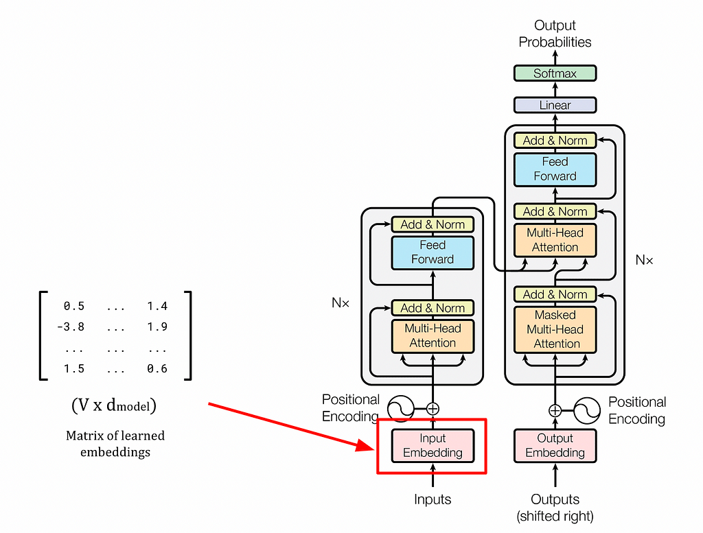
Much like the word2vec approach released four years prior, transformers store the initial vector representation for each token in the weights of a linear layer (a small neural network). In the word2vec model, these representations form the static embeddings, but in the Transformer context these are known as learned embeddings. In practice they are very similar, but using a different name emphasises that these representations are only a starting point for the transformer embeddings and not the final form.
The linear layer sits at the beginning of the Transformer architecture and contains only weights and no bias terms (bias = 0 for every neuron). The layer weights can be represented as a matrix of size V × d_model, where V is the vocabulary size (the number of unique words in the training data) and d_model is the number of embedding dimensions. In the previous article, we denoted d_model as N, in line with word2vec notation, but here we will use d_model which is more common in the Transformer context. The original Transformer was proposed with a d_model size of 512 dimensions, but in practice any reasonable value can be used.
A key difference between static and learned embeddings is the way in which they are trained. Static embeddings are trained in a separate neural network (using the Skip-Gram or Continuous Bag of Words architectures) using a word prediction task within a given window size. Once trained, the embeddings are then extracted and used with a range of different language models. Learned embeddings, however, are integral to the transformer you are using and are stored as weights in the first linear layer of the model. These weights, and consequently the learned embedding for each token in the vocabulary, are trained in the same backpropagation steps as the rest of the model parameters. Below is a summary of the training process for learned embeddings.
Step 1: Initialisation
Randomly initialise the weights for each neuron in the linear layer at the beginning of the model, and set the bias terms to 0. This layer is also called the embedding layer, since it is the linear layer that will store the learned embeddings. The weights can be represented as a matrix of size V × d_model, where the word embedding for each word in the vocabulary is stored along the rows. For example, the embedding for the first word in the vocabulary is stored in the first row, the second word is stored in the second row, and so on.
Step 2: Training
At each training step, the Transformer receives an input word and the aim is to predict the next word in the sequence — a task known as Next Token Prediction (NTP). Initially, these predictions will be very poor, and so every weight and bias term in the network will be updated to improve performance against the loss function, including the embeddings. After many training iterations, the learned embeddings should provide a strong vector representation for each word in the vocabulary.
Step 3: Extract the Learned Embeddings
When new input sequences are given to the model, the words are converted into tokens with an associated token ID, which corresponds to the position of the token in the tokenizer’s vocabulary. For example, the word cat may lie at position 349 in the tokenizer’s vocabulary and so will take the ID 349. Token IDs are used to create one-hot encoded vectors that extract the correct learned embeddings from the weights matrix (that is, V-dimensional vectors where every element is 0 except for the element at the token ID position, which is 1).
Note: PyTorch is a very popular deep learning library in Python that powers some of the most well-known machine learning packages, such as the HuggingFace Transformers library [2]. If you are familiar with PyTorch, you may have encountered the nn.Embedding class, which is often used to form the first layer of transformer networks (the nn denotes that the class belongs to the neural network package). This class returns a regular linear layer that is initialised with the identity function as the activation function and with no bias term. The weights are randomly initialised since they are parameters to be learned by the model during training. This essentially carries out the steps described above in one simple line of code. Remember, the nn.Embeddings layer does not provide pre-trained word embeddings out-of-the-box, but rather initialises a blank canvas of embeddings before training. This is to allow the transformer to learn its own embeddings during the training phase.
Once the learned embeddings have been trained, the weights in the embedding layer never change. That is, the learned embedding for each word (or more specifically, token) always provides the same starting point for a word’s vector representation. From here, the positional and contextual information will be added to produce a unique representation of the word that is reflective of its usage in the input sequence.
Transformer embeddings are created in a four-step process, which is demonstrated below using the example prompt: Write a poem about a man fishing on a river bank.. Note that the first two steps are the same as the word2vec approach we saw before. Steps 3 and 4 are the further processing that add contextual information to the embeddings.
Step 1) Tokenization:
Tokenization is the process of dividing a longer input sequence into individual words (and parts of words) called tokens. In this case, the sentence will be broken down into:
write, a, poem, about, a, man, fishing, on, a, river, bank
Next, the tokens are associated with their token IDs, which are integer values corresponding to the position of the token in the tokenizer’s vocabulary (see Part 1 of this series for an in-depth look at the tokenization process).
Step 2) Map the Tokens to Learned Embeddings:
Once the input sequence has been converted into a set of token IDs, the tokens are then mapped to their learned embedding vector representations, which were acquired during the transformer’s training. These learned embeddings have the “lookup table” behaviour as we saw in the word2vec example in Part 2 of this series. The mapping takes place by multiplying a one-hot encoded vector created from the token ID with the weights matrix, just as in the word2vec approach. The learned embeddings are denoted V in the image below.
Step 3) Add Positional Information with Positional Encoding:
Positional Encoding is then used to add positional information to the word embeddings. Whereas Recurrent Neural Networks (RNNs) process text sequentially (one word at a time), transformers process all words in parallel. This removes any implicit information about the position of each word in the sentence. For example, the sentences the cat ate the mouse and the mouse ate the cat use the same words but have very different meanings. To preserve the word order, positional encoding vectors are generated and added to the learned embedding for each word. In the image below, the positional encoding vectors are denoted P, and the sums of the learned embeddings and positional encodings are denoted X.
Step 4) Modify the Embeddings using Self-Attention:
The final step is to add contextual information using the self-attention mechanism. This determines which words give context to other words in the input sequence. In the image below, the transformer embeddings are denoted y.

Before the self-attention mechanism is applied, positional encoding is used to add information about the order of tokens to the learned embeddings. This compensates for the loss of positional information caused by the parallel processing used by transformers described earlier. There are many feasible approaches for injecting this information, but all methods must adhere to a set of constraints. The functions used to generate positional information must produce values that are:
These constraints ensure that the positional encoder produces positional information that allows words to attend to (gain context from) any other important word, regardless of their relative positions in the sequence. In theory, with a sufficiently powerful computer, words should be able to gain context from every relevant word in an infinitely long input sequence. The length of a sequence from which a model can derive context is called the context length. In chatbots like ChatGPT, the context includes the current prompt as well as all previous prompts and responses in the conversation (within the context length limit). This limit is typically in the range of a few thousand tokens, with GPT-3 supporting up to 4096 tokens and GPT-4 enterprise edition capping at around 128,000 tokens [3].
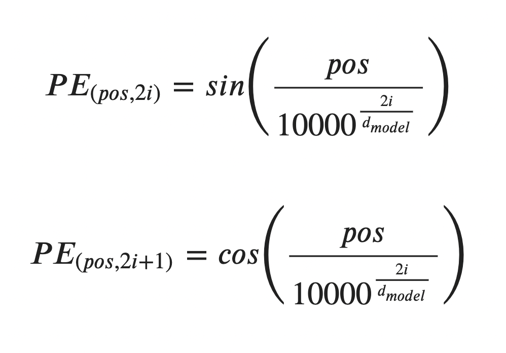
The original transformer model was proposed with the following positional encoding functions:
where:
The two proposed functions take arguments of 2i and 2i+1, which in practice means that the sine function generates positional information for the even-numbered dimensions of each word vector (i is even), and the cosine function does so for the odd-numbered dimensions (i is odd). According to the authors of the transformer:
“The positional encoding corresponds to a sinusoid. The wavelengths form a geometric progression from 2π to 10000·2π. We chose this function because we hypothesised it would allow the model to easily learn to attend by relative positions, since for any fixed offset k, PE_pos+k can be represented as a linear function of PE_pos”.
The value of the constant in the denominator being 10_000 was found to be suitable after some experimentation, but is a somewhat arbitrary choice by the authors.
The positional encodings shown above are considered fixed because they are generated by a known function with deterministic (predictable) outputs. This represents the most simple form of positional encoding. It is also possible to use learned positional encodings by randomly initialising some positional encodings and training them with backpropagation. Derivatives of the BERT architecture are examples of models that take this learned encoding approach. More recently, the Rotary Positional Encoding (RoPE) method has gained popularity, finding use in models such as Llama 2 and PaLM, among other positional encoding methods.
Creating a positional encoder class in Python is fairly straightforward. We can start by defining a function that accepts the number of embedding dimensions (d_model), the maximum length of the input sequence (max_length), and the number of decimal places to round each value in the vectors to (rounding). Note that transformers define a maximum input sequence length, and any sequence that has fewer tokens than this limit is appended with padding tokens until the limit is reached. To account for this behaviour in our positional encoder, we accept a max_length argument. In practice, this limit is typically thousands of characters long.
We can also exploit a mathematical trick to save computation. Instead of calculating the denominator for both PE_{pos, 2i} and PE_{pos, 2i}, we can note that the denominator is identical for consecutive pairs of i. For example, the denominators for i=0 and i=1 are the same, as are the denominators for i=2 and i=3. Hence, we can perform the calculations to determine the denominators once for the even values of i and reuse them for the odd values of i.
import numpy as np


class PositionalEncoder():
    """ An implementation of positional encoding.

    Attributes:
        d_model (int): The number of embedding dimensions in the learned
            embeddings. This is used to determine the length of the positional
            encoding vectors, which make up the rows of the positional encoding
            matrix.
        max_length (int): The maximum sequence length in the transformer. This
            is used to determine the size of the positional encoding matrix.
        rounding (int): The number of decimal places to round each of the
            values to in the output positional encoding matrix.
    """

    def __init__(self, d_model, max_length, rounding):
        self.d_model = d_model
        self.max_length = max_length
        self.rounding = rounding


    def generate_positional_encoding(self):
        """ Generate positional information to add to inputs for encoding.

        The positional information is generated using the number of embedding
        dimensions (d_model), the maximum length of the sequence (max_length),
        and the number of decimal places to round to (rounding). The output
        matrix generated is of size (max_length X embedding_dim), where each
        row is the positional information to be added to the learned
        embeddings, and each column is an embedding dimension.
        """

        position = np.arange(0, self.max_length).reshape(self.max_length, 1)
        even_i = np.arange(0, self.d_model, 2)
        denominator = 10_000**(even_i / self.d_model)

        even_encoded = np.round(np.sin(position / denominator), self.rounding)
        odd_encoded = np.round(np.cos(position / denominator), self.rounding)

        # Interleave the even and odd encodings
        positional_encoding = np.stack((even_encoded, odd_encoded),2)
        .reshape(even_encoded.shape[0],-1)

        # If self.d_model is odd remove the extra column generated
        if self.d_model % 2 == 1:
            positional_encoding = np.delete(positional_encoding, -1, axis=1)

        return positional_encoding


    def encode(self, input):
        """ Encode the input by adding positional information.

        Args:
            input (np.array): A two-dimensional array of embeddings. The array
                should be of size (self.max_length x self.d_model).

        Returns:
            output (np.array): A two-dimensional array of embeddings plus the
                positional information. The array has size (self.max_length x
                self.d_model).
        """
        positional_encoding = self.generate_positional_encoding()
        output = input + positional_encoding

        return output


MAX_LENGTH = 5
EMBEDDING_DIM = 3
ROUNDING = 2

# Instantiate the encoder
PE = PositionalEncoder(d_model=EMBEDDING_DIM,
                       max_length=MAX_LENGTH,
                       rounding=ROUNDING)

# Create an input matrix of word embeddings without positional encoding
input = np.round(np.random.rand(MAX_LENGTH, EMBEDDING_DIM), ROUNDING)

# Create an output matrix of word embeddings by adding positional encoding
output = PE.encode(input)

# Print the results
print(f'Embeddings without positional encoding:nn{input}n')
print(f'Positional encoding:nn{output-input}n')
print(f'Embeddings with positional encoding:nn{output}')
Embeddings without positional encoding:

[[0.12 0.94 0.9 ]
 [0.14 0.65 0.22]
 [0.29 0.58 0.31]
 [0.69 0.37 0.62]
 [0.25 0.61 0.65]]

Positional encoding:

[[ 0.    1.    0.  ]
 [ 0.84  0.54  0.  ]
 [ 0.91 -0.42  0.  ]
 [ 0.14 -0.99  0.01]
 [-0.76 -0.65  0.01]]

Embeddings with positional encoding:

[[ 0.12  1.94  0.9 ]
 [ 0.98  1.19  0.22]
 [ 1.2   0.16  0.31]
 [ 0.83 -0.62  0.63]
 [-0.51 -0.04  0.66]]
Recall that the positional information generated must be bounded, periodic, and predictable. The outputs of the sinusoidal functions presented earlier can be collected into a matrix, which can then be easily combined with the learned embeddings using element-wise addition. Plotting this matrix gives a nice visualisation of the desired properties. In the plot below, curving bands of negative values (blue) emanate from the left edge of the matrix. These bands form a pattern that the transformer can easily learn to predict.
import matplotlib.pyplot as plt

# Instantiate a PositionalEncoder class
d_model = 400
max_length = 100
rounding = 4

PE = PositionalEncoder(d_model=d_model,
                       max_length=max_length,
                       rounding=rounding)

# Generate positional encodings
input = np.round(np.random.rand(max_length, d_model), 4)
positional_encoding = PE.generate_positional_encoding()

# Plot positional encodings
cax = plt.matshow(positional_encoding, cmap='coolwarm')
plt.title(f'Positional Encoding Matrix ({d_model=}, {max_length=})')
plt.ylabel('Position of the Embeddingnin the Sequence, pos')
plt.xlabel('Embedding Dimension, i')
plt.gcf().colorbar(cax)
plt.gca().xaxis.set_ticks_position('bottom')

Now that we have covered an overview of transformer embeddings and the positional encoding step, we can turn our focus to the self-attention mechanism itself. In short, self-attention modifies the vector representation of words to capture the context of their usage in an input sequence. The “self” in self-attention refers to the fact that the mechanism uses the surrounding words within a single sequence to provide context. As such, self-attention requires all words to be processed in parallel. This is actually one of the main benefits of transformers (especially compared to RNNs) since the models can leverage parallel processing for a significant performance boost. In recent times, there has been some rethinking around this approach, and in the future we may see this core mechanism being replaced [4].
Another form of attention used in transformers is cross-attention. Unlike self-attention, which operates within a single sequence, cross-attention compares each word in an output sequence to each word in an input sequence, crossing between the two embedding matrices. Note the difference here compared to self-attention, which focuses entirely within a single sequence.
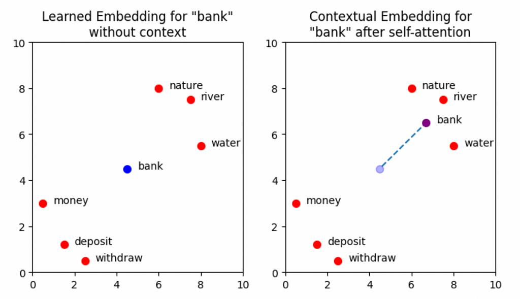
The plots below show a simplified set of learned embedding vectors in two dimensions. Words associated with nature and rivers are concentrated in the top right quadrant of the graph, while words associated with money are concentrated in the bottom left. The vector representing the word bank is positioned between the two clusters due to its polysemic nature. The objective of self-attention is to move the learned embedding vectors to regions of vector space that more accurately capture their meaning within the context of the input sequence. In the example input Write a poem about a man fishing on a river bank., the aim is to move the vector for bank in such a way that captures more of the meaning of nature and rivers, and less of the meaning of money and deposits.
Note: More accurately, the goal of self-attention here is to update the vector for every word in the input, so that all embeddings better represent the context in which they were used. There is nothing special about the word bank here that transformers have some special knowledge of — self-attention is applied across all the words. We will look more at this shortly, but for now, considering solely how bank is affected by self-attention gives a good intuition for what is happening in the attention block. For the purpose of this visualisation, the positional encoding information has not been explicitly shown. The effect of this will be minimal, but note that the self-attention mechanism will technically operate on the sum of the learned embedding plus the positional information and not solely the learned embedding itself.
import matplotlib.pyplot as plt

# Create word embeddings
xs = [0.5, 1.5, 2.5, 6.0, 7.5, 8.0]
ys = [3.0, 1.2, 0.5, 8.0, 7.5, 5.5]
words = ['money', 'deposit', 'withdraw', 'nature', 'river', 'water']
bank = [[4.5, 4.5], [6.7, 6.5]]

# Create figure
fig, ax = plt.subplots(ncols=2, figsize=(8,4))

# Add titles
ax[0].set_title('Learned Embedding for "bank"nwithout context')
ax[1].set_title('Contextual Embedding forn"bank" after self-attention')

# Add trace on plot 2 to show the movement of "bank"
ax[1].scatter(bank[0][0], bank[0][1], c='blue', s=50, alpha=0.3)
ax[1].plot([bank[0][0]+0.1, bank[1][0]],
           [bank[0][1]+0.1, bank[1][1]],
           linestyle='dashed',
           zorder=-1)

for i in range(2):
    ax[i].set_xlim(0,10)
    ax[i].set_ylim(0,10)

    # Plot word embeddings
    for (x, y, word) in list(zip(xs, ys, words)):
        ax[i].scatter(x, y, c='red', s=50)
        ax[i].text(x+0.5, y, word)

    # Plot "bank" vector
    x = bank[i][0]
    y = bank[i][1]

    color = 'blue' if i == 0 else 'purple'

    ax[i].text(x+0.5, y, 'bank')
    ax[i].scatter(x, y, c=color, s=50)
In the section above, we stated that the goal of self-attention is to move the embedding for each token to a region of vector space that better represents the context of its use in the input sequence. What we didn’t discuss is how this is done. Here we will show a step-by-step example of how the self-attention mechanism modifies the embedding for bank, by adding context from the surrounding tokens.
Step 1) Calculate the Similarity Between Words using the Dot Product:
The context of a token is given by the surrounding tokens in the sentence. Therefore, we can use the embeddings of all the tokens in the input sequence to update the embedding for any word, such as bank. Ideally, words that provide significant context (such as river) will heavily influence the embedding, while words that provide less context (such as a) will have minimal effect.
The degree of context one word contributes to another is measured by a similarity score. Tokens with similar learned embeddings are likely to provide more context than those with dissimilar embeddings. The similarity scores are calculated by taking the dot product of the current embedding for one token (its learned embedding plus positional information) with the current embeddings of every other token in the sequence. For clarity, the current embeddings have been termed self-attention inputs in this article and are denoted x.
There are several options for measuring the similarity between two vectors, which can be broadly categorised into: distance-based and angle-based metrics. Distance-based metrics characterise the similarity of vectors using the straight-line distance between them. This calculation is relatively simple and can be thought of as applying Pythagoras’s theorem in d_model-dimensional space. While intuitive, this approach is computationally expensive.
For angle-based similarity metrics, the two main candidates are: cosine similarity and dot-product similarity. Both of these characterise similarity using the cosine of the angle between the two vectors, θ. For orthogonal vectors (vectors that are at right angles to each other) cos(θ) = 0, which represents no similarity. For parallel vectors, cos(θ) = 1, which represents that the vectors are identical. Solely using the angle between vectors, as is the case with cosine similarity, is not ideal for two reasons. The first is that the magnitude of the vectors is not considered, so distant vectors that happen to be aligned will produce inflated similarity scores. The second is that cosine similarity requires first computing the dot product and then dividing by the product of the vectors’ magnitudes — making cosine similarity a computationally expensive metric. Therefore, the dot product is used to determine similarity. The dot product formula is given below for two vectors x_1 and x_2.

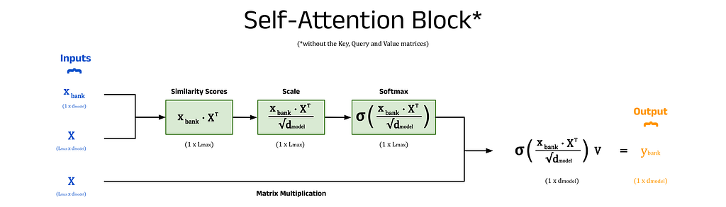
The diagram below shows the dot product between the self-attention input vector for bank, x_bank, and the matrix of vector representations for every token in the input sequence, X^T. We can also write x_bank as x_11 to reflect its position in the input sequence. The matrix X stores the self-attention inputs for every token in the input sequence as rows. The number of columns in this matrix is given by L_max, the maximum sequence length of the model. In this example, we will assume that the maximum sequence length is equal to the number of words in the input prompt, removing the need for any padding tokens (see Part 4 in this series for more about padding). To compute the dot product directly, we can transpose X and calculate the vector of similarity scores, S_bank using S_bank = x_bank ⋅ X^T. The individual elements of S_bank represent the similarity scores between bank and each token in the input sequence.

Step 2) Scale the Similarity Scores:
The dot product approach lacks any form of normalisation (unlike cosine similarity), which can cause the similarity scores to become very large. This can pose computational challenges, so normalisation of some form becomes necessary. The most common method is to divide each score by √d_model, resulting in scaled dot-product attention. Scaled dot-product attention is not restricted to self-attention and is also used for cross-attention in transformers.
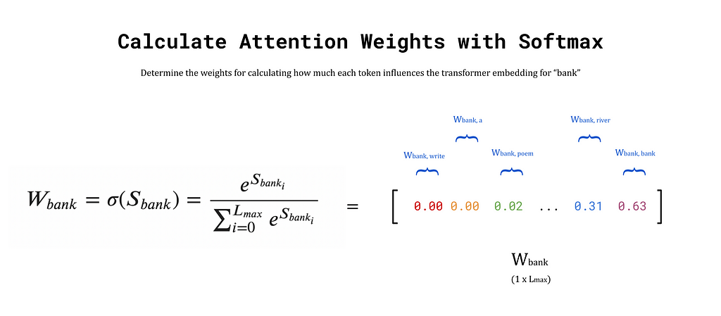
Step 3) Calculate the Attention Weights using the Softmax Function:
The output of the previous step is the vector S_bank, which contains the similarity scores between bank and every token in the input sequence. These similarity scores are used as weights to construct a transformer embedding for bank from the weighted sum of embeddings for each surrounding token in the prompt. The weights, known as attention weights, are calculated by passing S_bank into the softmax function. The outputs are stored in a vector denoted W_bank. To see more about the softmax function, refer to the previous article on word2vec.
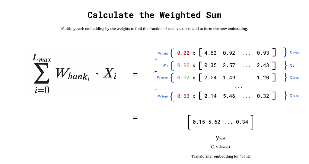
Step 4) Calculate the Transformer Embedding
Finally, the transformer embedding for bank is obtained by taking the weighted sum of write, a, prompt, …, bank. Of course, bank will have the highest similarity score with itself (and therefore the largest attention weight), so the output embedding after this process will remain similar to before. This behaviour is ideal since the initial embedding already occupies a region of vector space that encodes some meaning for bank. The goal is to nudge the embedding towards the words that provide more context. The weights for words that provide little context, such as a and man, are very small. Hence, their influence on the output embedding will be minimal. Words that provide significant context, such as river and fishing, will have higher weights, and therefore pull the output embedding closer to their regions of vector space. The end result is a new embedding, y_bank, that reflects the context of the entire input sequence.
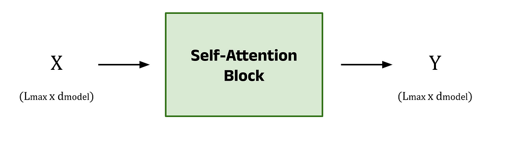
Above, we walked through the steps to calculate the transformer embedding for the singular word bank. The input consisted of the learned embedding vector for bank plus its positional information, which we denoted x_11 or x_bank. The key point here, is that we considered only one vector as the input. If we instead pass in the matrix X (with dimensions L_max × d_model) to the self-attention block, we can calculate the transformer embedding for every token in the input prompt simultaneously. The output matrix, Y, contains the transformer embedding for every token along the rows of the matrix. This approach is what enables transformers to quickly process text.
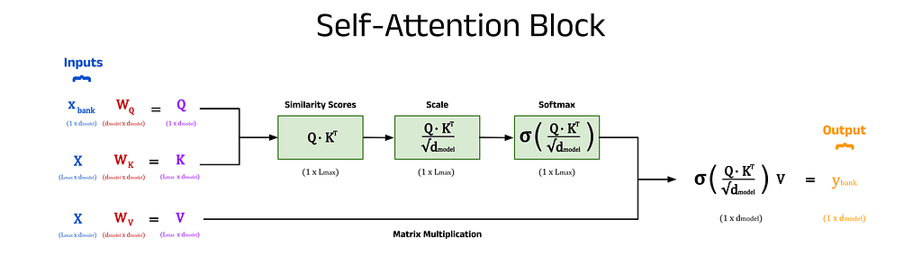
The above description gives an overview of the core functionality of the self-attention block, but there is one more piece of the puzzle. The simple weighted sum above does not include any trainable parameters, but we can introduce some to the process. Without trainable parameters, the performance of the model may still be good, but by allowing the model to learn more intricate patterns and hidden features from the training data, we observe much stronger model performance.
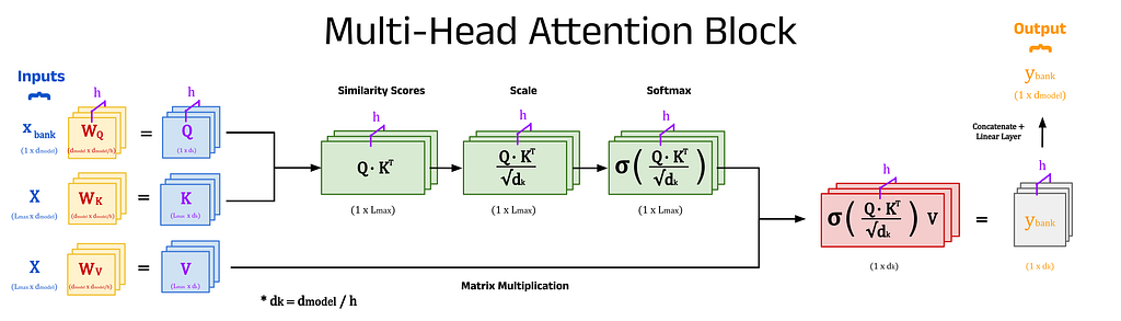
The self-attention inputs are used three times to calculate the new embeddings, these include the x_bank vector, the X^T matrix in the dot product step, and the X^T matrix in the weighted sum step. These three sites are the perfect candidates to introduce some weights, which are added in the form of matrices (shown in red). When pre-multiplied by their respective inputs (shown in blue), these form the key, query, and value matrices, K, Q, and V (shown in purple). The number of columns in these weight matrices is an architectural choice by the user. Choosing a value for d_q, d_k, and d_v that is less than d_model will result in dimensionality reduction, which can improve model speed. Ultimately, these values are hyperparameters that can be changed based on the specific implementation of the model and the use-case, and are often all set equal to d_model if unsure [5].
The names for these matrices come from an analogy with databases, which is explained briefly below.
Query:
Key:
Value:
Distributing Computation Across Multiple Heads:
The “Attention is All You Need” paper expands self-attention into multi-head attention, which gives even richer representations of the input sequences. This method involves repeating the calculation of attention weights using different key, query, and value matrices which are learned independently within each head. A head is a section of the attention block dedicated to processing a fraction of the input embedding dimensions. For example, an input, x, with 512 dimensions will be divided by the number of heads, h, to create h chunks of size d_k (where d_k = d_model / h). For a model with 8 heads (h=8), each head will receive 64 dimensions of x (d_k = 64). Each chunk is processed using the self-attention mechanism in its respective head, and at the end the outputs from all heads are combined using a linear layer to produce a single output with the original 512 dimensions.
The Benefits of Using Multiple Heads:
The core idea is to allow each head to learn different types of relationships between words in the input sequence, and to combine them to create deep text representations. For example, some heads might learn to capture long-term dependencies (relationships between words that are distant in the text), while others might focus on short-term dependencies (words that are close in text).
Building Intuition for Multi-Head Attention:
To build some intuition for the usefulness of multiple attention heads, consider words in a sentence that require a lot of context. For example, in the sentence I ate some of Bob’s chocolate cake, the word ate should attend to I, Bob’s and cake to gain full context. This is a rather simple example, but if you extend this concept to complex sequences spanning thousands of words, hopefully it seems reasonable that distributing the computational load across separate attention mechanisms will be beneficial.

Summary of Multi-Head Attention:
To summarise, multi-head attention involves repeating the self-attention mechanism h times and combining the results to distil the information into rich transformer embeddings. While this step is not strictly necessary, it has been found to produce more impressive results, and so is standard in transformer-based models.
Python has many options for working with transformer models, but none are perhaps as well-known as Hugging Face. Hugging Face provides a centralised resource hub for NLP researchers and developers alike, including tools such as:
The code cell below shows how the transformers library can be used to load a transformer-based model into Python, and how to extract both the learned embeddings for words (without context) and the transformer embeddings (with context). The remainder of this article will break down the steps shown in this cell and describe additional functionalities available when working with embeddings.
import torch
from transformers import AutoModel, AutoTokenizer


def extract_le(sequence, tokenizer, model):
    """ Extract the learned embedding for each token in an input sequence.

    Tokenize an input sequence (string) to produce a tensor of token IDs.
    Return a tensor containing the learned embedding for each token in the
    input sequence.

    Args:
        sequence (str): The input sentence(s) to tokenize and extract
            embeddings from.
        tokenizer: The tokenizer used to produce tokens.
        model: The model to extract learned embeddings from.

    Returns:
        learned_embeddings (torch.tensor): A tensor containing tensors of
            learned embeddings for each token in the input sequence.
    """
    token_dict = tokenizer(sequence, return_tensors='pt')
    token_ids = token_dict['input_ids']
    learned_embeddings = model.embeddings.word_embeddings(token_ids)[0]

    # Additional processing for display purposes
    learned_embeddings = learned_embeddings.tolist()
    learned_embeddings = [[round(i,2) for i in le]
                          for le in learned_embeddings]

    return learned_embeddings


def extract_te(sequence, tokenizer, model):
    """ Extract the tranformer embedding for each token in an input sequence.

    Tokenize an input sequence (string) to produce a tensor of token IDs.
    Return a tensor containing the transformer embedding for each token in the
    input sequence.

    Args:
        sequence (str): The input sentence(s) to tokenize and extract
            embeddings from.
        tokenizer: The tokenizer used to produce tokens.
        model: The model to extract learned embeddings from.

    Returns:
        transformer_embeddings (torch.tensor): A tensor containing tensors of
            transformer embeddings for each token in the input sequence.
    """
    token_dict = tokenizer(sequence, return_tensors='pt')

    with torch.no_grad():
        base_model_output = model(**token_dict)

    transformer_embeddings = base_model_output.last_hidden_state[0]

    # Additional processing for display purposes
    transformer_embeddings = transformer_embeddings.tolist()
    transformer_embeddings = [[round(i,2) for i in te]
                              for te in transformer_embeddings]

    return transformer_embeddings


# Instantiate DistilBERT tokenizer and model
tokenizer = AutoTokenizer.from_pretrained('distilbert-base-uncased')
model = AutoModel.from_pretrained('distilbert-base-uncased')

# Extract the learned embedding for bank from DistilBERT
le_bank = extract_le('bank', tokenizer, model)[1]

# Write sentences containing "bank" in two different contexts
s1 = 'Write a poem about a man fishing on a river bank.'
s2 = 'Write a poem about a man withdrawing money from a bank.'

# Extract the transformer embedding for bank from DistilBERT in each sentence
s1_te_bank = extract_te(s1, tokenizer, model)[11]
s2_te_bank = extract_te(s2, tokenizer, model)[11]

# Print the results
print('------------------- Embedding vectors for "bank" -------------------n')
print(f'Learned embedding:                  {le_bank[:5]}')
print(f'Transformer embedding (sentence 1): {s1_te_bank[:5]}')
print(f'Transformer embedding (sentence 2): {s2_te_bank[:5]}')
------------------- Embedding vectors for "bank" -------------------

Learned embedding:                  [-0.03, -0.06, -0.09, -0.07, -0.03]
Transformer embedding (sentence 1): [0.15, -0.16, -0.17, -0.08, 0.44]
Transformer embedding (sentence 2): [0.27, -0.23, -0.23, -0.21, 0.79]
The first step to produce transformer embeddings is to choose a model from the Hugging Face transformers library. In this article, we will not use the model for inference but solely to examine the embeddings it produces. This is not a standard use-case, and so we will have to do some extra digging in order to access the embeddings. Since the transformers library is written in PyTorch (referred to as torch in the code), we can import torch to extract data from the inner workings of the models.
For this example, we will use DistilBERT, a smaller version of Google’s BERT model which was released by Hugging Face themselves in October 2019 [6]. According to the Hugging Face documentation [7]:
DistilBERT is a small, fast, cheap and light Transformer model trained by distilling BERT base. It has 40% less parameters than bert-base-uncased, runs 60% faster while preserving over 95% of BERT’s performances as measured on the GLUE language understanding benchmark.
We can import DistilBERT and its corresponding tokenizer into Python either directly from the transformers library or using the AutoModel and AutoTokenizer classes. There is very little difference between the two, although AutoModel and AutoTokenizer are often preferred since the model name can be parameterised and stored in a string, which makes it simpler to change the model being used.
import torch
from transformers import DistilBertTokenizerFast, DistilBertModel

# Instantiate DistilBERT tokenizer and model
tokenizer = DistilBertTokenizerFast.from_pretrained('distilbert-base-uncased')
model = DistilBertModel.from_pretrained('distilbert-base-uncased')
import torch
from transformers import AutoModel, AutoTokenizer

# Instantiate DistilBERT tokenizer and model
tokenizer = AutoTokenizer.from_pretrained('distilbert-base-uncased')
model = AutoModel.from_pretrained('distilbert-base-uncased')
After importing DistilBERT and its corresponding tokenizer, we can call the from_pretrained method for each to load in the specific version of the DistilBERT model and tokenizer we want to use. In this case, we have chosen distilbert-base-uncased, where base refers to the size of the model, and uncased indicates that the model was trained on uncased text (all text is converted to lowercase).
Next, we can create some sentences to give the model some words to embed. The two sentences, s1 and s2, both contain the word bank but in different contexts. The goal here is to show that the word bank will begin with the same learned embedding in both sentences, then be modified by DistilBERT using self-attention to produce a unique, contextualised embedding for each input sequence.
# Create example sentences to produce embeddings for
s1 = 'Write a poem about a man fishing on a river bank.'
s2 = 'Write a poem about a man withdrawing money from a bank.'
The tokenizer class can be used to tokenize an input sequence (as shown below) and convert a string into a list of token IDs. Optionally, we can also pass a return_tensors argument to format the token IDs as a PyTorch tensor (return_tensors=pt) or as TensorFlow constants (return_tensors=tf). Leaving this argument empty will return the token IDs in a Python list. The return value is a dictionary that contains input_ids: the list-like object containing token IDs, and attention_mask which we will ignore for now.
Note: BERT-based models include a [CLS] token at the beginning of each sequence, and a [SEP] token to distinguish between two bodies of text in the input. These are present due to the tasks that BERT was originally trained on and can largely be ignored here. For a discussion on BERT special tokens, model sizes, cased vs uncased, and the attention mask, see Part 4 of this series.
token_dict = tokenizer(s1, return_tensors='pt')
token_ids = token_dict['input_ids'][0]
Each transformer model provides access to its learned embeddings via the embeddings.word_embeddings method. This method accepts a token ID or collection of token IDs and returns the learned embedding(s) as a PyTorch tensor.
learned_embeddings = model.embeddings.word_embeddings(token_ids)
learned_embeddings
tensor([[ 0.0390, -0.0123, -0.0208,  ...,  0.0607,  0.0230,  0.0238],
        [-0.0300, -0.0070, -0.0247,  ...,  0.0203, -0.0566, -0.0264],
        [ 0.0062,  0.0100,  0.0071,  ..., -0.0043, -0.0132,  0.0166],
        ...,
        [-0.0261, -0.0571, -0.0934,  ..., -0.0351, -0.0396, -0.0389],
        [-0.0244, -0.0138, -0.0078,  ...,  0.0069,  0.0057, -0.0016],
        [-0.0199, -0.0095, -0.0099,  ..., -0.0235,  0.0071, -0.0071]],
       grad_fn=<EmbeddingBackward0>)
Converting a context-lacking learned embedding into a context-aware transformer embedding requires a forward pass of the model. Since we are not updating the weights of the model here (i.e. training the model), we can use the torch.no_grad() context manager to save on memory. This allows us to pass the tokens directly into the model and compute the transformer embeddings without any unnecessary calculations. Once the tokens have been passed into the model, a BaseModelOutput is returned, which contains various information about the forward pass. The only data that is of interest here is the activations in the last hidden state, which form the transformer embeddings. These can be accessed using the last_hidden_state attribute, as shown below, which concludes the explanation for the code cell shown at the top of this section.
with torch.no_grad():
    base_model_output = model(**token_dict)

transformer_embeddings = base_model_output.last_hidden_state
transformer_embeddings
tensor([[[-0.0957, -0.2030, -0.5024,  ...,  0.0490,  0.3114,  0.1348],
         [ 0.4535,  0.5324, -0.2670,  ...,  0.0583,  0.2880, -0.4577],
         [-0.1893,  0.1717, -0.4159,  ..., -0.2230, -0.2225,  0.0207],
         ...,
         [ 0.1536, -0.1616, -0.1735,  ..., -0.3608, -0.3879, -0.1812],
         [-0.0182, -0.4264, -0.6702,  ...,  0.3213,  0.5881, -0.5163],
         [ 0.7911,  0.2633, -0.4892,  ..., -0.2303, -0.6364, -0.3311]]])
It is possible to convert token IDs back into textual tokens, which shows exactly how the tokenizer divided the input sequence. This is useful when longer or rarer words are divided into multiple subwords when using subword tokenizers such as WordPiece (e.g. in BERT-based models) or Byte-Pair Encoding (e.g. in the GPT family of models).
tokens = tokenizer.convert_ids_to_tokens(token_ids)
tokens
['[CLS]', 'write', 'a', 'poem', 'about', 'a', 'man', 'fishing', 'on', 'a',
 'river', 'bank', '.', '[SEP]']
The self-attention mechanism generates rich, context-aware transformer embeddings for text by processing each token in an input sequence simultaneously. These embeddings build on the foundations of static word embeddings (such as word2vec) and enable more capable language models such as BERT and GPT. Further work in this field will continue to improve the capabilities of LLMs and NLP as a whole.
[1] A. Vaswani, N. Shazeer, N. Parmar, J. Uszkoreit, L. Jones, A. N. Gomez, Ł. Kaiser, and I. Polosukhin, Attention is All You Need (2017), Advances in Neural Information Processing Systems 30 (NIPS 2017)
[2] Hugging Face, Transformers (2024), HuggingFace.co
[3] OpenAI, ChatGPT Pricing (2024), OpenAI.com
[4] A. Gu and T. Dao, Mamba: Linear-Time Sequence Modelling with Selective State Spaces (2023), ArXiv abs/2312.00752
[5] J. Alammar, The Illustrated Transformer (2018). GitHub
[6] V. Sanh, L. Debut, J. Chaumond, and T. Wolf, DistilBERT, a distilled version of BERT: smaller, faster, cheaper and lighter (2019), 5th Workshop on Energy Efficient Machine Learning and Cognitive Computing — NeurIPS 2019
[7] Hugging Face, DistilBERT Documentation (2024) HuggingFace.co
[8] Hugging Face, BERT Documentation (2024) HuggingFace.co
Self-Attention Explained with Code was originally published in Towards Data Science on Medium, where people are continuing the conversation by highlighting and responding to this story.
Originally appeared here:
Self-Attention Explained with Code
Go Here to Read this Fast! Self-Attention Explained with Code


With a little over a year since the launch of ChatGPT, it is clear that public perception of “AI” has shifted dramatically. Part of this is a by-product of increased general awareness but it has more so been influenced by the realization that AI-powered systems may be (already are?) capable of human-level competence and performance. In many ways, ChatGPT has served as a proof-of-concept demonstration for AI as a whole. The work on this demonstration kicked off more than a half century ago and has now yielded compelling evidence that we are closer to a reality where we can ‘create machines that perform functions that require intelligence when performed by people,’ to borrow Ray Kurzweil’s definition. It should be no surprise then that the discussions and development around AI Agents have exploded in recent months. They are the embodiment of aspirations that AI has always aimed for.
To be clear, the concept of AI agents is by no means a new one. Our imaginations have been there many times over — C-3PO of Star Wars fame is embodied AI at its finest, capable of human-level natural language comprehension, dialogue, and autonomous action. In the more formal setting of academics, Norvig and Russell’s textbook on AI, Artificial Intelligence: A Modern Approach, states that intelligent agents are the main unifying theme. The ideas around AI agents, whether born in science or fiction, all seem a bit more realizable with the arrival of models like ChatGPT, Claude, and Gemini, which are broadly competent in diverse knowledge domains and equipped with strong comprehension and capability for human-level dialogue. Add in new capabilities like “vision” and function calling, and the stage is set for the proliferation of AI agent development.
As we barrel down the path toward the development of AI agents, it seems necessary to begin transitioning from prompt engineering to something broader, a.k.a. agent engineering, and establishing the appropriate frameworks, methodologies, and mental models to design them effectively. In this article, I set out to explore some of the key ideas and precepts of agent engineering within the LLM context.
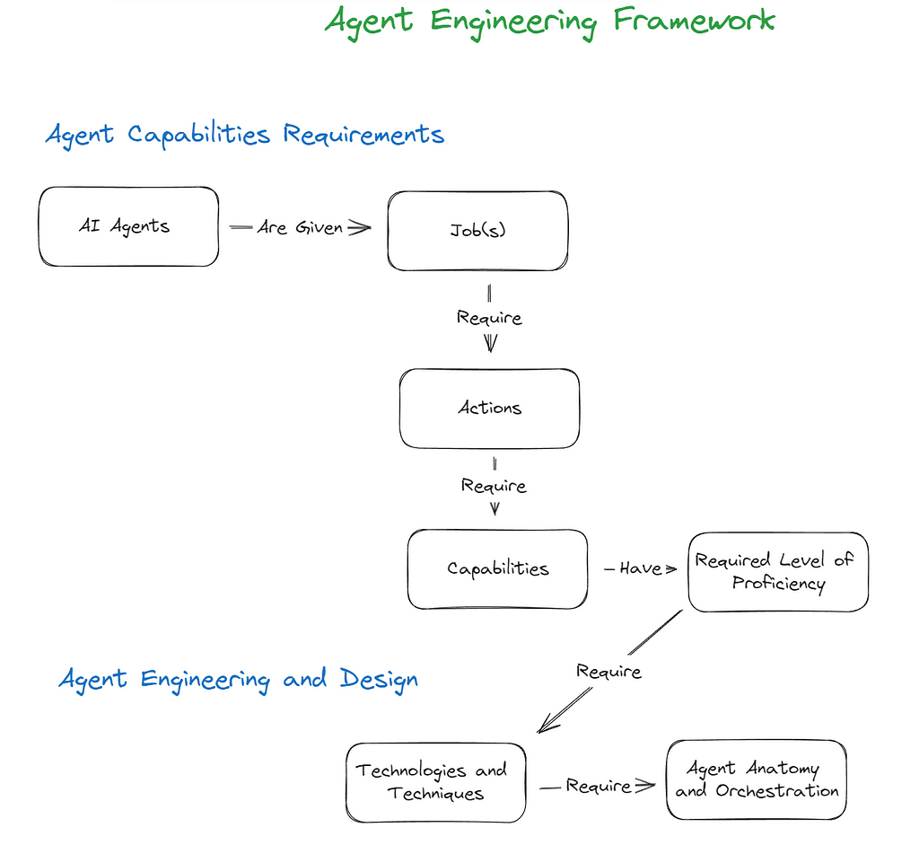
Let’s explore on a high level the key sections of the Agent Engineering Framework. We begin with the ‘Agent Capabilities Requirements,’ where we aim to clearly define what the agent needs to do and how proficient it needs to be. In ‘Agent Engineering and Design,’ we evaluate the technologies available to us and begin thinking through the anatomy and orchestration of our agent(s).
This early-stage articulation of the framework is intended to be a practical mental model and is admittedly not comprehensive on all fronts. But I believe there is value in starting somewhere and then refining and enhancing over time.
Introduction
What is the purpose of building an AI agent? Does it have a job or a role? Actions in support of goals? Or goals in support of actions? Is a multi-capability agent better than a multi-agent swarm for a particular job? The beauty of human language is that it is flexible and allows us to metaphorically extend concepts in many directions. The downside to this is that can lead to ambiguity. In articulating the framework, I am purposefully trying to avoid parsing semantic distinctions between key terms, since many of them can be used interchangeably. We strive instead to surface concepts that generalize in their application to AI Agent Engineering broadly. As a result the framework at this stage is more of a mental model that aims to guide the thought process around Agent Engineering. The core ideas are relatively straightforward as you can see in the below graphic:
Agent Capabilities Requirements
The Job to be Done
The initial step in designing an AI agent is to clearly outline what the agent is supposed to do. What are the primary jobs, tasks or goals the agent needs to accomplish? This could be framed as a high-level objective or broken down into specific jobs and tasks. You may decide to use a multi-agent swarm approach and assign each agent a task. The language and level of detail can vary. For example:
Note that in both of these cases, labels such as jobs, tasks, goals, etc. could be used interchangeably within the context of what the agent is supposed to do.
The Actions to Take to Perform the Job
Once the jobs to be done are defined, the next step is to determine the specific actions the agent needs to perform relative to that job. The focus moves from simply defining what the agent is supposed to achieve to specifying how it will get done through concrete actions. At this stage it is also important to begin considering the appropriate level of autonomy for the agent. For instance:
For a content creation agent, the actions might include:
The content creation agent might autonomously generate and draft content, with a human editor providing final approval. Or a separate agent editor may be employed to do a first review before a human editor gets involved.
The Capabilities Needed
Now that we have outlined the actions that our agents need to take to perform the job(s) we proceed to articulating the capabilities needed to enable those actions. They can include everything from natural language dialogue, information retrieval, content generation, data analysis, continuous learning and more. They can also be expressed on a more technical level such as API calls, function calls etc. For example for our content creation agent the desired capabilities might be:
It is important ultimately to focus on expressing the capabilities in ways that do not constrain the choices and eventual selection of which technologies to work with. For example, although we all are all quite enamored with LLMs, Large Action Models (LAMs) are evolving quickly and may be relevant for enabling the desired capabilities.
Required Proficiency Level of the Capabilities
While identifying the capabilities necessary for an agent to perform its job is a crucial step, it is equally important to assess and define the proficiency level required for each of these capabilities. This involves setting specific benchmarks and performance metrics that must be met for the agent and its capabilities to be considered proficient. These benchmarks can include accuracy, efficiency, and reliability.
For example, for our content creation agent, desired proficiency levels might include:
Agent Engineering & Design
Mapping Required Proficiencies to Technologies and Techniques
Once the needed capabilities and required proficiency levels are specified, the next step is to determine how we can meet these requirements. This involves evaluating a fast growing arsenal of available technologies and techniques including LLMs, RAG, Guardrails, specialized APIs, and other ML/AI models to assess if they can achieve the specified proficiency levels. In all cases it is helpful to consider what any given technology or technique is best at on a high-level and the cost/benefit implications. I will superficially discuss a few here but it will be limited in scope and scale as there are myriad possibilities.
Broad Knowledge Proficiency
Broad knowledge refers to the general understanding and information across a wide range of topics and domains. This type of knowledge is essential for creating AI agents that can effectively engage in dialogue, understand context, and provide relevant responses across various subjects.
Specific Knowledge Proficiency
Specific knowledge involves a deeper understanding of particular domains or topics. This type of knowledge is necessary for tasks that require detailed expertise and familiarity with specialized content. What technologies/techniques might we consider as we aim at our proficiency targets?
Precise Information
Precise information refers to highly accurate and specific data points that are critical for tasks requiring exact answers.
Agent Anatomy and Orchestration
Now that we have a firm grasp of what the Agent’s job is, the capabilities and proficiency levels required and the technologies available to enable them, we shift our focus to the anatomy and orchestration of the agent either in a solo configuration or some type of swarm or ecosystem. Should capabilities be registered to one agent, or should each capability be assigned to a unique agent that operates within a swarm? How do we develop capabilities and agents that can be re-purposed with minimum effort? This topic alone involves multiple articles and so we won’t dive into it further here. In some respects this is where the “rubber meets the road” and we find ourselves weaving together multiple technologies and techniques to breathe life into our Agents.
The journey from Prompt Engineering to Agent Engineering is just beginning, and there is much to learn and refine along the way. This first stab at an Agent Engineering Framework proposes a practical approach to designing AI agents by outlining a high-level mental model that can serve as a useful starting point in that evolution. The models and techniques available for building Agents will only continue to proliferate, creating a distinct need for frameworks that generalize away from any one specific technology or class of technologies. By clearly defining what an agent needs to do, outlining the actions required to perform these tasks, and specifying the necessary capabilities and proficiency levels, we set a strong and flexible foundation for our design and engineering efforts. It further provides a structure for our agents and their capabilities to be improved and evolve over time.
Thanks for reading and I hope you find the Agent Engineering Framework helpful in you agent oriented endeavors. Stay tuned for future refinements of framework and elaborations on various topics mentioned. If you would like to discuss the framework or other topics I have written about further, do not hesitate to connect with me on LinkedIn.
Unless otherwise noted, all images in this article are by the author.
From Prompt Engineering to Agent Engineering was originally published in Towards Data Science on Medium, where people are continuing the conversation by highlighting and responding to this story.
Originally appeared here:
From Prompt Engineering to Agent Engineering
Go Here to Read this Fast! From Prompt Engineering to Agent Engineering


Exploring the Differences and Use Cases of Shiny Core and Shiny Express for Python
Originally appeared here:
Understanding the Two Faces of Shiny for Python: Core and Express
Go Here to Read this Fast! Understanding the Two Faces of Shiny for Python: Core and Express
Because data scientists don’t write production code in the Udemy code editor
Originally appeared here:
Data Scientists Work in the Cloud. Here’s How to Practice This as a Student (Part 2: Python)

“What gets measured gets managed” was coined by Peter Drucker, regarded as the father of modern management, in 1954. It is an often quoted saying which is actually part of a larger, and I think more powerful quote “What gets measured gets managed — even when it’s pointless to measure and manage it, and even if it harms the purpose of the organization to do so.”
Drucker’s insight underscores that, while gathering and measuring data is essential, the real challenge lies in identifying and prioritizing the right metrics that will drive a business in the right direction. By focusing on and prioritizing the right metrics, you can ensure that what gets measured and managed is truly impactful.
This blog focuses on product analytics in technology companies, however this idea rings true for all businesses and types of analytics. Below is a summary of what I’ve learnt and applied working as a data professional in a start-up (Digivizer), a scale-up (Immutable), and a big tech company (Facebook) across a range of different products.
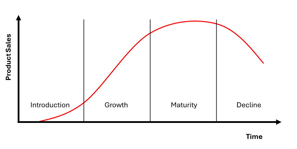
The most important metrics for a company change over time. Uber was not profitable for around 15 years, yet the company is considered one of the most successful businesses in recent time. Why? Uber focused intensely on rapid growth in its initial years rather than immediate profitability. The company prioritized metrics like user growth and user retention to establish a dominant presence in the ride-sharing market. Then, once Uber became the dominant ride-sharing company, its focus shifted towards profitability and financial sustainability. It, like many others, anchored their metrics to the stages of the product lifecycle.
You should prioritize metrics based on the product lifecycle stages.
The metrics you focus on during each stage should help answer the urgent problems that each stage presents. The tactical problems can vary but will derive from the following high level questions:
The first and most crucial stage in the product lifecycle is the Introduction stage, where the primary focus is on achieving product-market-fit. At this stage, product owners must determine whether their product meets a genuine market need and resonates with the target audience. Understanding product-market-fit involves assessing whether early adopters are not only using the product but also finding value in it. Being confident in product-market-fit sets the foundation for future growth and scalability.
There are 3 metrics that can provide clarity on whether you have achieved product-market-fit. These are, in order of importance:
Used together, these three metrics can quantitatively measure whether there is product-market-fit or point to the most critical product issue. There are 5 potential scenarios you will fall into:
Once an organization has confidence in product-market-fit, the attention can shift to growth. This approach avoids spending large amounts on user acquisition only to have to pivot the product or market, or have the majority of users churn.
The Growth stage is where a product has the potential to move from promising to dominant. A perfect example of effective scaling is Facebook’s famous “8 friends in 10 days” rule. By using funnel analysis and experimentation, Facebook discovered that new users who connected with at least 8 friends within their first 10 days were far more likely to remain active on the platform. This insight led to focused efforts on optimizing user onboarding and encouraging friend connections, significantly boosting user retention and stickiness. In this stage, the key question is: how do we scale effectively while maintaining product quality and user satisfaction?
Analytics in this stage should broaden to include 3 types:
When implementing user journey analysis, less is more. The temptation may be to instrument every page and every button in a product, but this can often be onerous for engineering to implement and difficult to maintain. Instead, start with just a beginning and end event — these two events will allow you to calculate a conversion rate and a time to convert. Expand beyond two events to only include critical steps in a user journey. Ensure that events capture user segments such as device, operating system and location.
Experimentation is a muscle that requires exercise. You should start building this capability early in a product and company’s lifecycle because it is more difficult to implement than a set of metrics. Build the muscle by involving product, engineering and data teams in experiment design. Experimentation is not only crucial in ‘Stage 2 — Growth’ but should remain a fundamental part of analytics throughout the rest of the product lifecycle.
‘Aha’ Analysis helps identify pivotal moments that can turbocharge growth. These are the key interactions where users realize the product’s value, leading to loyalty and stickiness. Facebook’s 8 friends in 10 days was their users ‘aha’ moment. This analysis requires analysts to explore a variety of potential characteristics and can be difficult to identify and distil down to a simple ‘aha’ moment. Be sure to use the hypothesis driven approach to avoid boiling the ocean.
In the Maturity stage, the focus shifts from rapid growth to optimizing for profitability and long-term sustainability. This phase is about refining the product, maximizing efficiency, and ensuring the business remains competitive. Companies like Apple, Netflix and Amazon have successfully navigated this stage by honing in on cost management, increasing user revenue, and exploring new revenue streams.
Focus in this stage shifts to:
Monetization metrics have clear objectives in terms of trying to increase revenue and decrease costs. Marketing and Go-To-Market teams often own CAC reduction and product teams often own LTV and MRR improvement. Strategies can range from optimizing advertising spend, reducing time to close sales deals through to cross-selling and bundling products for existing users. Broadly, a LTV:CAC ratio of 3:1 to 4:1 is often used as a target for B2B software companies while B2C targets are closer to 2.5:1.
“Your margin is my opportunity” — Jeff Bezos. As products mature, profitability inevitably declines. Competitors identify your opportunity and increase competition, existing users migrate to substitutes and new technologies, and markets become saturated, offering little growth. In this phase, maintaining the existing user base becomes paramount.
In Stage 4, there are a broad set of useful metrics that can be adopted. Some key types are:
By creating churn prediction models and analyzing the feature importance, characteristics of users who are likely to churn can be identified and intervention measures deployed. Given new user growth has slowed, retaining existing users is critical. This analysis may also help resurrect previously churned users too.
Power user analysis seeks to understand the most engaged users and their characteristics. These users are the highest priority to retain, and have the product-usage behavior that would ideally be shared across all users. Look for users active every day, who spend long periods of time in the product, who use the most features and who spend the most. Deploy measures, such as loyalty programs, to retain these users and identify pathways to increase the number of power users.
Root cause analysis is essential for delving into specific problem areas within a mature product. Given the complexity and scale of products at this lifecycle stage, having the capability to conduct bespoke deep dives into issues is vital. This type of analysis helps uncover the underlying drivers of key metrics, provides confidence in product changes that are costly to implement and can help untangle the interdependent measures across the product ecosystem.
A product or company who finds themselves in this final stage may choose to create new products and enter new markets. At that point, the cycle begins again and the focus shifts back to product-market-fit at the start of this blog.
“Focus is about saying no.” — Steve Jobs. Product analytics is a bottomless pit of potential metrics, dimensions and visualizations. To effectively use product analytics, companies must prioritize metrics down to a few focus areas at any one time. These metrics can be supported by a range of other measures, but must have the following:
This can be achieved by prioritizing the right metrics at each product lifecycle stage — Introduction, Growth, Maturity, and Decline. From achieving product-market fit to scaling effectively, optimizing for profitability, and maintaining user interest, each phase demands a clear focus on the most relevant problems to solve.
Remember, it’s not about measuring everything; it’s about measuring what matters. In the words of Steve Jobs, let’s say no to the noise and yes to what truly drives our products forward.
I avoided listing too many specific metrics in the sections above and only provided some example metrics for each product lifecycle stage. Instead I focused on the over-arching themes to focus analytics against. But, if you are looking for the long list of options, there are some good resources linked below.
Your End-to-End Product Analytics Strategy was originally published in Towards Data Science on Medium, where people are continuing the conversation by highlighting and responding to this story.
Originally appeared here:
Your End-to-End Product Analytics Strategy
Go Here to Read this Fast! Your End-to-End Product Analytics Strategy

Text classification models aren’t new, but the bar for how quickly they can be built and how well they perform has improved.
The transformer-based model I will fine-tune here is more than 1000 times smaller than GPT-3.5 Turbo. It will perform consistently better for this use case because it will be specifically trained for it.
The idea is to optimize AI workflows where smaller models excel, particularly in handling redundant tasks where larger models are simply overkill.
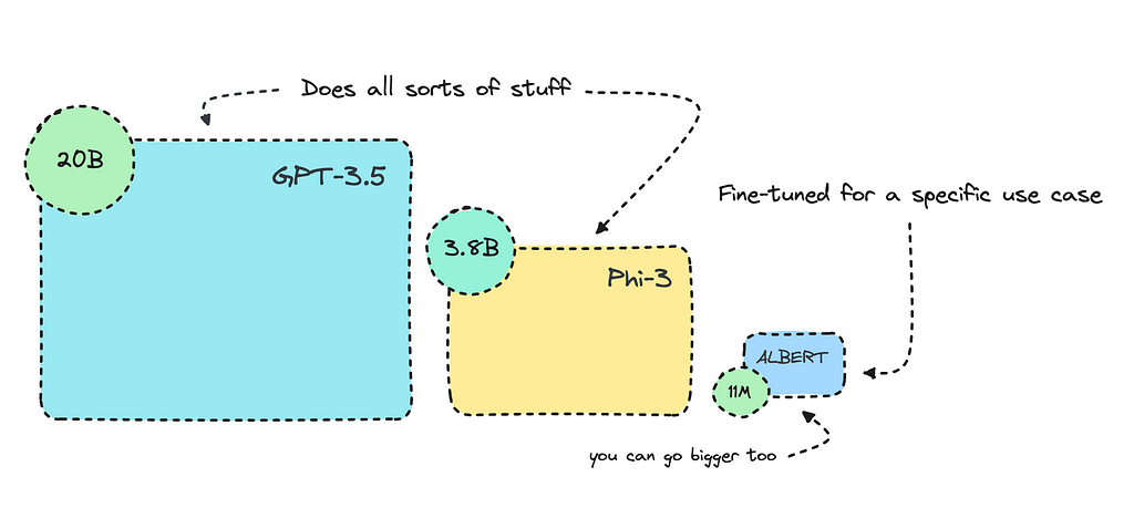
I’ve previously talked about this, where I built a slightly larger keyword extractor for tech-focused content using a sequence-to-sequence transformer model. I also went through the different models and what they excelled at.
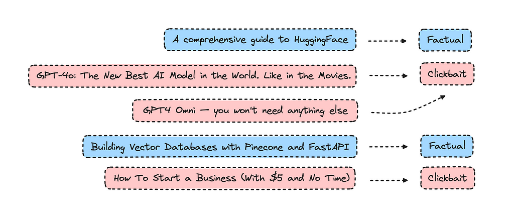
For this piece, I’m diving into text classification with transformers, where encoder models do well. I’ll train a pre-trained encoder model with binary classes to identify clickbait versus factual articles. However, you may train it for a different use case.
You’ll find the finished model here.
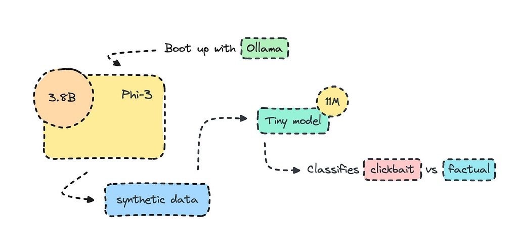
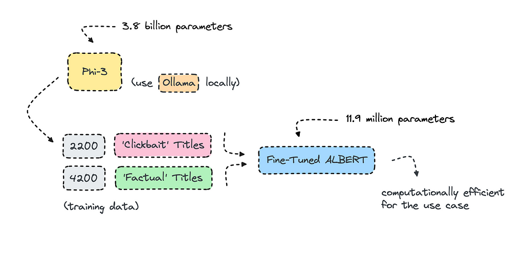
Most organizations use open-source LLMs such as Mistral and Llama to transform their datasets for training, but what I’ll do here is create the training data altogether using Phi-3 via Ollama.
There is always the risk that the model will overfit when using data from a large language model, but in this case, it performed fine, so I’m getting on the artificial data train. However, you will have to be careful and look at the metrics once it is in training.
As for building a text classifier to identify clickbait titles, I think we can agree that some clickbait can be good as it keeps things interesting. I tried the finished model on various titles I made up, and found that having only factual content can be a bit dull.
These issues always seem clear-cut, then you dive into them, and they are more nuanced than you considered. The question that popped into my head was, ‘What’s good clickbait content versus bad clickbait content?’ A platform will probably need a bit of both to keep people reading.
I used the new model on all my own content, and none of my titles were identified as clickbait. I’m not sure if that’s something good or not.
If you’re new to transformer encoder models like BERT, this is a good learning experience. If you are not new to building text classification models with transformers, you might find it interesting to see if synthetic data worked well and to look at my performance metrics for this model.
As we all know, it’s easier to use fake data than to access the real thing.
I got inspiration for this piece from Fabian Ridder as he was using ChatGPT to identify clickbait and factual articles to train a model using FastText. I thought this case would be great for a smaller transformer model.
The model we’re building will use synthetic data rather than the real thing, though. The process will be quick, as it will only take about an hour or so to generate data with Phi-3 and a few minutes to train it. The model will be very small, with only 11M parameters.
As we’re using binary classes, i.e., clickbait or factual, we will be able to achieve 99% accuracy. The model will have the ability to interpret nuanced texts much better than FastText though.
The cost of training will be zero, and I have already prepared the dataset that we’ll use for this. However, you may generate your own data for another use case.
If you want to dive into training the model, you can skip the introduction where I provide some information on encoder models and the tasks they excel in.
While transformers have introduced amazing capabilities in generating text, they have also improved within other NLP tasks, such as text classification and extraction.
The distinction between model architectures is a bit blurry but it’s useful to understand that different transformer models were originally built for different tasks.
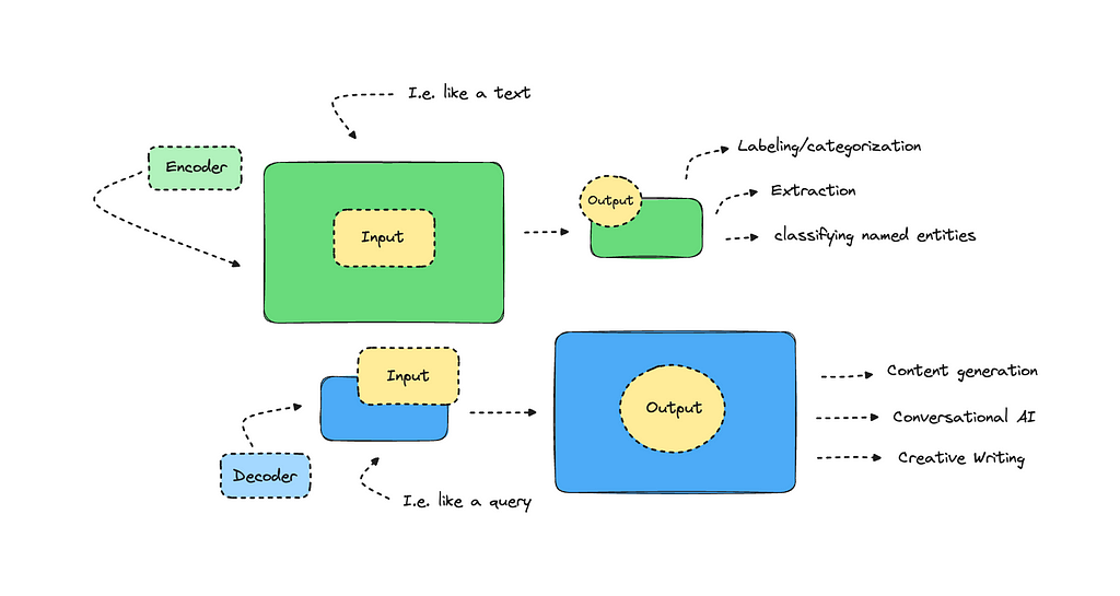
A decoder model takes in a smaller input and outputs a larger text. GPT, which introduced impressive text generation back when, is a decoder model. While larger language models offer more nuanced capabilities today, decoders were not built for tasks that involve extraction and labeling. For these tasks, we can use encoder models, which take in more input and provide a condensed output.
Encoders excel at extracting information rather than generating it.
I won’t go into it any more than this, but there should be a lot of information you can scout on the topic, albeit it can be a bit technical.
So, what tasks are popular with encoders? Some examples include sentiment analysis, categorization, named entity recognition, and keyword/topic extraction, among others.
You can try a model that classifies text into twelve different emotions here. You can also look into a model that classifies hate speech as toxic here. Both of these were built with an encoder-only model, in this case, RoBERTa.
There are many base models you can work with; RoBERTa is a newer model that used more data for training and improved on BERT by optimizing its training techniques.
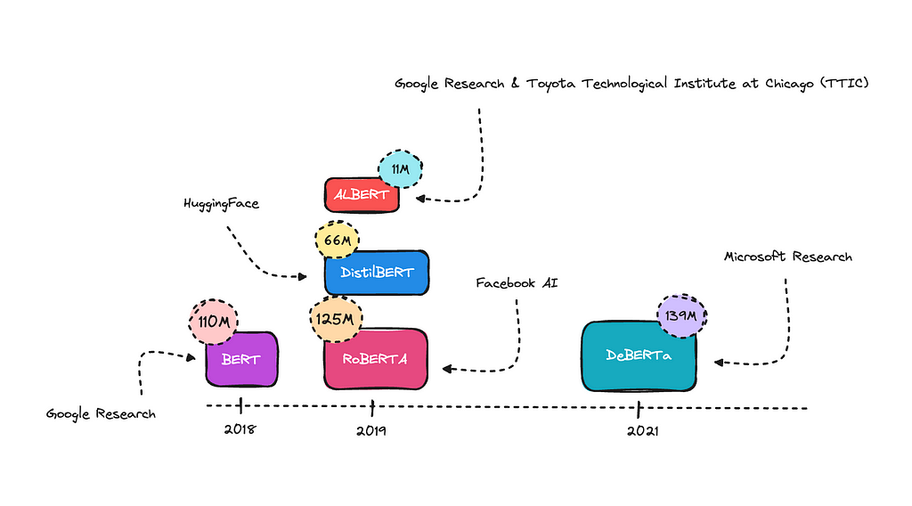
BERT was the first encoder-only transformer model, this one started it all by understanding language context much better than previous models. DistillBERT is a compressed version of BERT.
ALBERT uses some tricks to reduce the number of parameters, making it smaller without significantly losing performance. This is the one I’ll use for this case, as I think it will do well.
DeBERTA is an improved model that better understands word relationships and context. Generally, the bigger models will perform better on complex NLP tasks. However, they can more easily overfit if the training data is not diverse enough.
For this piece, I’m focusing on one task: text classification. So, how hard is it to build a text classification model? It really depends on what you are asking it to do. When working with binary classes, you can achieve a high accuracy score in most cases. However, it also depends on how complex the use case is.
There are certain benchmarks you can look at to understand how BERT has performed with different open-source datasets. I reviewed the paper “How to Fine-Tune BERT for Text Classification?” to look at these benchmarks and graphed their accuracy score with the amount of labels they were trained with below.
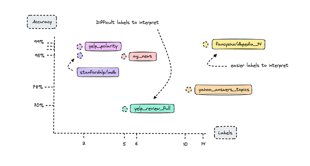
We see datasets with only two labels do quite well. This is what we call binary labels. What might stand out is the DBpedia dataset, which has 14 classes, yet achieved 98% accuracy as a benchmark, whereas the Yelp Review Full dataset, with only 5 classes, achieved only 70%.
Here’s where complexity comes in: Yelp reviews are very difficult to label, especially when rating stars between 1 and 5. Think about how difficult it is for a human to classify someone else’s text into a specific star rating; it really depends on how the person classifies their own reviews.
If you were to build a text classifier with the Yelp reviews dataset, you would find that 1-star and 5-star reviews are labeled correctly most of the time, but the model would struggle with 2, 3, and 4-star reviews. This is because what one person may classify as a 2-star review, the AI model might interpret as a 3-star review.
The DBpedia dataset on the other hand has texts that are easier to interpret for the model.
When we train a model, we can look at the metrics per label rather than as a whole to understand which labels are underperforming. Nevertheless, if you are working with a complex task, don’t feel discouraged if your metrics aren’t perfect.
Always try it afterwards on new data to see if it works well enough on your use case and keep working on the dataset, or switch the underlying model.
I always have a section on the cost of building and running a model. In any project, you’ll have to weigh resources and efficiency to get an outcome.
If you are just trying things out, then a bigger model with an API endpoint makes sense even though it will be computationally inefficient.
I have been running Claude Haiku to do natural language processing for a project now for a month, extracting category, topics and location from texts. This is for demonstration purposes only, but it makes sense when you want to prototype something for an organization.
However, doing zero-shot with these bigger models, will result in a lot of inconsistency, and some texts have to be disregarded altogether. Sometimes the bigger models will output absolute gibberish, but at the same time, it’s cheaper to run them for such a small project.
With your own models you will also have to host them, that’s why we spend so much time trying to make them smaller. You can naturally run them locally, but you’ll probably want to be able to use them for a development project so you’ll need to keep hosting costs in consideration.
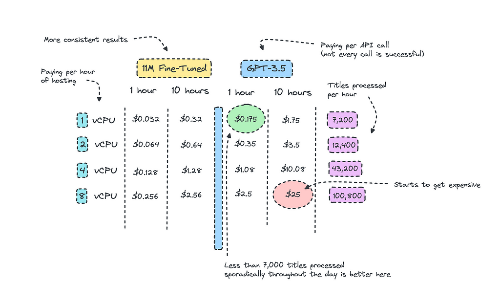
Looking at the picture up top, I have calculated the amount of titles we can process for each instance and compared the same costs for GPT-3.5. I’m aware that it may look a bit messy, but alas it is hard to vizualise.
We can at least deduce that if we are sporadically using GPT-3.5 throughout the day for a small project, it makes sense to use it even though the costs to host the smaller model is quite low.
The breakpoint is when you are consistently processing so much data that surpasses a certain threshold. For this case, this would be when the titles to be processed exceeds 32,000 per day as the cost to keep the instance running 24/7 would equal the same price.
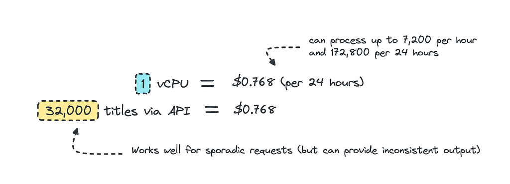
This calculates as if you are keeping the instance running throughout the day, if you are only processing data at certain hours of the day, it makes sense to host and then scale down to zero when it is not in use. Since it’s so small, we can also just containerize it and then host it on ECS or even Lambda for serverless inference.
When using the closed sourced LLMs for zero-shot inference, we would also need to take into account that the model hasn’t been trained for this specific case so we may get inconsistent results. So for redundant tasks where you need consistency, building your own model is a better choice.
It is also worth noting that sometimes you need models that perform on more complex tasks. Here, the cost difference might be steeper for the larger LLMs as you’ll need a better model and a longer prompt template.
Transforming data with the use of LLMs isn’t new, if you’re not doing it you should. This is much faster than manually transforming thousands of data points.
I looked at what Orange, the telecom giant, had done via their AI/NLP task force — NEPAL — and they had grabbed data from various places and transformed the raw texts into instruction-like formats using GPT-3.5 and Mixtral to create data that could be used for training.
If you’re keen to read more on this you can look at the session that is provided via Nvidia’s GTC here.
But people are going further than this, using the larger language models to build the entire dataset; this is called synthetic data. It’s a smart way to build smaller specialized models with data that comes from the larger language models but that are cheaper and more efficient to host.
There are concerns at this though, where the quality of synthetic data can be questioned. Relying only on generated data might lead to models that miss nuances or biases inherent in real world data causing it to malfunction when it actually sees it.
However, it is much easier to generate synthetic data than to access the real thing.
I will embark on creating a very simple model here, the model is simply to identify titles as either clickbait or factual. You may build a different text classifier with more labels.
The process is straightforward and I’ll go through the entire process, the cook book we’ll work with is this one.
This tutorial will use this dataset, if you want to build your own dataset be sure to read the first section.
To create a synthetic dataset, we can boot up Ollama locally and run a model we want to use to build the training data. Make sure it is a commercially available model. I chose Phi-3, because it is small and it is very good.
I quite like Javascript, so I used the Ollama JS framework to build a script that could run in the background to produce a CSV file.
This script creates clickbait titles and stores it in a new CSV in your root folder. You need to change the prompt template later to produce an equal amount of titles that are factual.
As I’m using a generative text model, Phi-3, some outputs won’t be usable, but that is to be expected. It will take some time for this to run, so go do something else with your time.
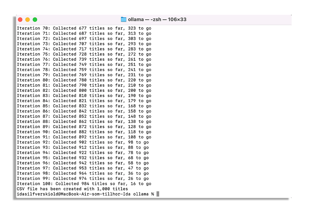
Once you’re finished you can store your finished CSV file with the clickbait and factual tiles in your Google Drive. Remember to set the text and label as fields, where the text is the title and the label is whether it is clickbait or factual.

Since I’ve already prepared the dataset we’ll use, please see this script to upload your custom dataset to HuggingFace.
Looking through the dataset, you’ll see that most clickbait articles that have been generated by Phi-3 has an exclamation mark at the end of it. This is something you want to make sure doesn’t happen, so it’s important to check the work of the LLM generating the data.
Remember that the script I provided you with splits your data into a training, test and validation set. I would recommend to have at least a training and test set for training the model.
If you’ve got your dataset sorted, we can go ahead and fine-tune the model.
If you haven’t opened up the cook book, do so here. The first part of this is deciding on your dataset and then your pre-trained model.
from datasets import load_dataset, DatasetDict

dataset = load_dataset("ilsilfverskiold/clickbait_titles_synthetic_data")
dataset
model_name = "albert/albert-base-v2"
your_path = "classify-clickbait"
I wen’t through the different models under the introduction section, where ALBERT and DistillBERT are smaller models and BERT and RoBERTa are larger.
For this case, as it’s not overly complex, I will go for ALBERT. I’m sure BERT can do better, but ALBERT is ten times smaller. RoBERTa is too big and may produce some overfitting with this dataset.
Remember, if you’re working with a different language then look for a base model that has been trained on a corpus from at least a similar language.
If you’re working with nordic languages I can recommend KB/bert-base-swedish-cased that I used to create a model for the IPTC newscodes categories.
Now we need to do a few things for this to work well.
We first convert our labels to a standardized numerical format that the trainer will understand.
from sklearn.preprocessing import LabelEncoder

label_encoder = LabelEncoder()

label_encoder.fit(dataset['train']['label'])

def encode_labels(example):
    return {'encoded_label': label_encoder.transform([example['label']])[0]}

for split in dataset:
    dataset[split] = dataset[split].map(encode_labels, batched=False)
Then we need to map the numerical representations back to the actual label names. This is so we can get the actual label names rather than the numerical reps when we do inference with the model.
from transformers import AutoConfig

unique_labels = sorted(list(set(dataset['train']['label'])))
id2label = {i: label for i, label in enumerate(unique_labels)}
label2id = {label: i for i, label in enumerate(unique_labels)}

config = AutoConfig.from_pretrained(model_name)
config.id2label = id2label
config.label2id = label2id

# Verify the correct labels
print("ID to Label Mapping:", config.id2label)
print("Label to ID Mapping:", config.label2id)
After this we’re ready to fetch the pre-trained model and it’s tokenizer. We use the config we set up with the labels when we import the model.
from transformers import AlbertForSequenceClassification, AlbertTokenizer

tokenizer = AlbertTokenizer.from_pretrained(model_name)
model = AlbertForSequenceClassification.from_pretrained(model_name, config=config)
If you’re using a different model such as BERT or RoBERTa, you can use AutoTokenizer and AutoModelForSequenceClassification which will automatically select the correct classes for your specified model.
This next function filters for invalid content and then makes sure the text data is properly tokenized and labeled, preparing the dataset for training.
def filter_invalid_content(example):
    return isinstance(example['text'], str)

dataset = dataset.filter(filter_invalid_content, batched=False)

def encode_data(batch):
    tokenized_inputs = tokenizer(batch["text"], padding=True, truncation=True, max_length=256)
    tokenized_inputs["labels"] = batch["encoded_label"]
    return tokenized_inputs

dataset_encoded = dataset.map(encode_data, batched=True)
dataset_encoded
dataset_encoded.set_format(type='torch', columns=['input_ids', 'attention_mask', 'labels'])
We also need to fetch a data collator to handle padding for our inputs.
from transformers import DataCollatorWithPadding

data_collator = DataCollatorWithPadding(tokenizer)
It’s not required for you to set up any evaluation metrics, such as accuracy, precision, recall or f1. However, you do need at least accuracy to understand how the model is performing.
Accuracy measures the amount of predictions the model got right across all categories. Precision measures how often predictions for a specific category are correct. Recall tells us how well the model can identify all instances within a specific category. The F1 Score is the weighted average of Precision and Recall.
I won’t go into detail on these metrics, but there are many others that write about this. For this case, I’m more interested in how it performs on new real data rather than synthetic data. So, what I look out for are metrics that are too good, indicating that it has overfitted.
We do though set up a function that let us look at the accuracy for each label rather than as an average. This is much more relevant when you have many labels, rather than just two.
from sklearn.preprocessing import LabelEncoder
from sklearn.metrics import accuracy_score, confusion_matrix
import numpy as np

label_encoder = LabelEncoder()
label_encoder.fit(unique_labels)

def per_label_accuracy(y_true, y_pred, labels):
    cm = confusion_matrix(y_true, y_pred, labels=labels)
    correct_predictions = cm.diagonal()
    label_totals = cm.sum(axis=1)
    per_label_acc = np.divide(correct_predictions, label_totals, out=np.zeros_like(correct_predictions, dtype=float), where=label_totals != 0)
    return dict(zip(labels, per_label_acc))
We also set up the general compute metrics function. I am using all of these metrics here because this is general template I have for any text classifier, but you may decide which ones you want.
from sklearn.metrics import accuracy_score, recall_score, precision_score, f1_score

def compute_metrics(pred):
    labels = pred.label_ids
    preds = pred.predictions.argmax(-1)

    decoded_labels = label_encoder.inverse_transform(labels)
    decoded_preds = label_encoder.inverse_transform(preds)

    precision = precision_score(decoded_labels, decoded_preds, average='weighted')
    recall = recall_score(decoded_labels, decoded_preds, average='weighted')
    f1 = f1_score(decoded_labels, decoded_preds, average='weighted')
    acc = accuracy_score(decoded_labels, decoded_preds)

    labels_list = list(label_encoder.classes_)
    per_label_acc = per_label_accuracy(decoded_labels, decoded_preds, labels_list)

    per_label_acc_metrics = {}
    for label, accuracy in per_label_acc.items():
        label_key = f"accuracy_label_{label}"
        per_label_acc_metrics[label_key] = accuracy

    return {
        'accuracy': acc,
        'f1': f1,
        'precision': precision,
        'recall': recall,
        **per_label_acc_metrics
    }
Once you’re decently satisfied, we can move on to setting up the training arguments and the trainer.
Next up we set up our training arguments. Here you can tweak the epochs, batch size and learning rate.
from transformers import Trainer, TrainingArguments

training_args = TrainingArguments(
    output_dir=your_path,
    num_train_epochs=3,
    warmup_steps=500,
    per_device_train_batch_size=16,
    per_device_eval_batch_size=16,
    weight_decay=0.01,
    logging_steps=10,
    evaluation_strategy='steps',
    eval_steps=100,
    learning_rate=2e-5,
    save_steps=1000,
    gradient_accumulation_steps=2
)
I chose to go with a learning rate and epochs based on the paper “How to Fine-Tune BERT for Text Classification?” but decreased the batch size.
Now we can go ahead and set up the trainer, with everything we’ve prepared, and run it.
trainer = Trainer(
    model=model,
    args=training_args,
    train_dataset=dataset_encoded['train'],
    eval_dataset=dataset_encoded['test'],
    compute_metrics=compute_metrics,
    tokenizer=tokenizer,
    data_collator=data_collator,
)

trainer.train()
When in training, you need to look out for overfitting. As both the training and evaluation datasets are synthetic, the typical signs of overfitting might be unclear.
Keep an eye on the accuracy and loss for both the training and evaluation datasets. I.e. very low training and validation loss, along with too stellar evaluation metrics could be a sign of overfitting.
But remember binary classes with less complex tasks usually perform well.
You’ll see my results for one run I made below.
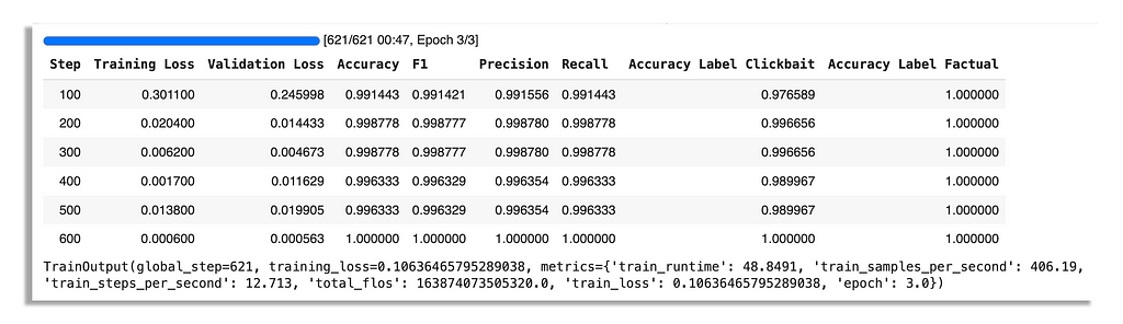
As you can see from the training metrics, they are a bit too good. Validation loss is fluctuating as well. This could be a very bad sign so you have to make sure to test the model on real data once it has finished training.
If you’re training a model with several classes, perhaps even with a skewed dataset, don’t worry if the average evaluation metrics aren’t great. Look at the metrics per label.
Once it’s done training, you can run the final evaluation metrics, save the model and then save the state. This will build the metrics for when you push it to the hub for your model page.
trainer.evaluate()
trainer.save_model(your_path)
trainer.save_state()
Now you can run the HuggingFace pipeline in your notebook to test it.
from transformers import pipeline
pipe = pipeline('text-classification', model=your_path)
example_titles = [
    "grab an example title",
    "grab another example title",
    "and another xample title"
]

for title in example_titles:
    result = pipe(title)
    print(f"Title: {title}")
    print(f"Output: {result[0]['label']}")
Mine did fine on test data, however it missed a few clickbait articles that I personally found to be clickbait. For a production use case, it’s better to build a more diverse dataset (especially with synthetic data) so it can perform well on new real data.
Nevertheless, if you’re not satisfied, then you go back to the dataset, redo it or try with a different model.
If you are wondering, I have indeed gotten stellar results on some runs and less-than-stellar results on other runs with the same data, the same training parameters, and the same seed.
Before you push the model, you can also test the model against other alternatives.
I asked GPT-3.5 to tell me which titles it thought was clickbait and factual, and it did really well which is to be expected, it is more than 1000x larger than Albert.
We can also compare some titles to what a fine-tuned FastText says versus the fine-tuned transformer encoder model.
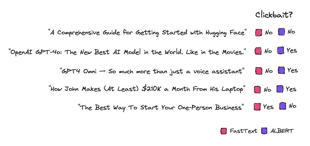
Using FastText is very simple and computationally efficient, but it treats words in isolation and lacks deep contextual understanding.
Therefore, FastText doesn’t capture the context and nuances of language as well as a model that is transformer based.
If you’re satisfied with your model, you can push it to the HuggingFace hub to store it there.
You simply login with a write token you can find in your HuggingFace account under Settings.
!huggingface-cli login
And then push it.
tokenizer.push_to_hub("username/classify-clickbait")
trainer.push_to_hub("username/classify-clickbait")
Push the tokenizer just in case, especially if you are working with a version of Albert.
Now you can use it directly from there, mine you’ll find there.
If you want to use a larger model like BERT, you can apply different techniques so you can distill it further after fine-tuning. I didn’t find it that much more successful than just using ALBERT, at least for this case.
BERT on its own though performed much better in general. Although I really like RoBERTa for most cases, it was prone to overfit on this specific dataset either because it was too small, not good enough or too artificial.
For every case you’ll have to estimate how much performance you can sacrifice for efficiency and eventually you learn which models do well in what situation.
Would the model have performed better if we had used real data? It’s possible, but the accuracy may be lower unless the dataset is meticulously sorted.
This is hard work.
Using synthetic data can get the job done very quickly so you get up a prototype to work with. Synthetic data is much cleaner to work with.
You are also free to work with the larger open source LLMs, so it doesn’t break any rules for people that can’t access high quality data without breaching protocol.
I did not put down time and effort into building this dataset, but in all cases you should make sure you have varied data the model can learn from.
Hopefully this piece was useful and gave you some inspiration and ideas on how to work with the smaller models.
❤
Fine-Tune Smaller Transformer Models: Text Classification was originally published in Towards Data Science on Medium, where people are continuing the conversation by highlighting and responding to this story.
Originally appeared here:
Fine-Tune Smaller Transformer Models: Text Classification
Go Here to Read this Fast! Fine-Tune Smaller Transformer Models: Text Classification

Did you know that the same dataset can be graphically represented differently based on the audience we have in front of us? This is because each audience has different requirements, meaning that each audience will look for something different in the data. Recognizing what the audience is looking for in a graph becomes essential to building graphs adapted to that type of audience.
We will cover:
Let’s start from the beginning. We consider three fundamental audience types:
The following figure shows the various types of audiences and their specific objectives.
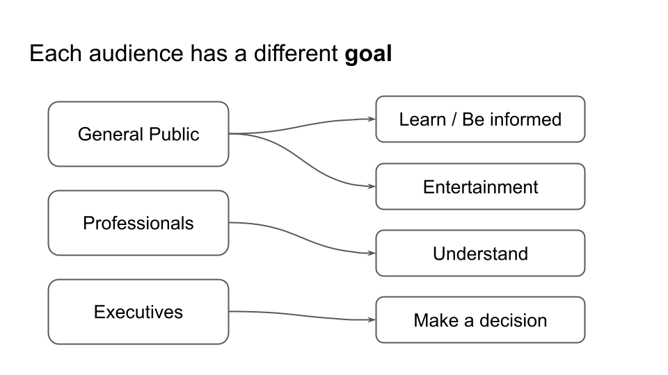
In this article, we will focus on the professional audience. In the next ones, we will analyze the other types of audiences. We will use an example dataset and build a chart specifically targeted to this audience. Showing the same graphic produced to a different kind of audience would probably only have a negative effect and reduce the level of understanding of the message.
As already mentioned, professionals know the topic very well and want to understand the data better. Therefore, the more data details we include in the graph, the more we satisfy their needs. In this case, in fact, it is better to give specific values of the data, without rounding too much.
Including some elements in the graph that invite them to reflect, carry out calculations, or discuss is also appropriate. For example, professionals may be interested in:
What do we want our audience of professionals to do?
In summary, for this type of audience, we provide the following information in a graph:
We use the Global Temperature Anomalies dataset released by NOAA under the Creative Commons 1.0 Universal Public Domain Dedication (CC0–1.0) license. We build a graph specific to the professional audience to represent the dataset. As a graph construction tool, we use Python Altair, but you can generalize and also use other tools such as Tableau, Power BI, or Matplotlib.
We will follow the steps described below:
Start by loading the dataset, which is not ready for usage because the date is incorrect. Data preprocessing is outside the scope of data visualization, but here, we report the code for conversion just for convenience.
import pandas as pd

df = pd.read_csv('source/1850-2024.csv')
The following figure shows the output:
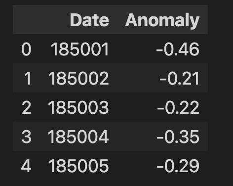
Define a function for conversion, which takes the year from the first four characters of the cell and the date from the next two characters:
# Function to convert YYYYMM to YYYY-MM-DD
def convert_to_date(yyyymm):
    year = int(str(yyyymm)[:4])
    month = int(str(yyyymm)[4:6])
    return pd.Timestamp(year=year, month=month, day=1)

# Apply the conversion function to the Date column
df['Date'] = df['Date'].apply(convert_to_date)
The first thing we can do is draw the raw chart to know what data we have. Use a line to represent the data, as shown in the following code:
import altair as alt

chart = alt.Chart(df
).mark_line(
).encode(
    x='Date',
    y='Anomaly'
).properties(
    width=800
)

chart
The following figure shows the resulting chart:
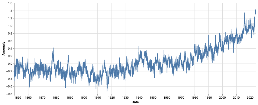
We have a very basic chart that shows the anomaly in temperatures from 1850 to 2023. The represented value is not a temperature but an anomaly of temperature in degrees. For example, in 1850, the anomaly was 0.4 degrees under the expected value, which is set to 0. This basic chart needs to be clarified.
Let’s improve the basic chart by tailoring it to the professional audience.
Professionals are very technical people who already know the topic and want to understand the data-related details.
To tailor the chart for professionals, start by transforming the chart into a bar chart, by simply using the mark_bar() function.
chart = alt.Chart(df
).mark_bar(
).encode(
    x='Date',
    y='Anomaly'
).properties(
    width=900
)

chart
The following figure shows the resulting chart.
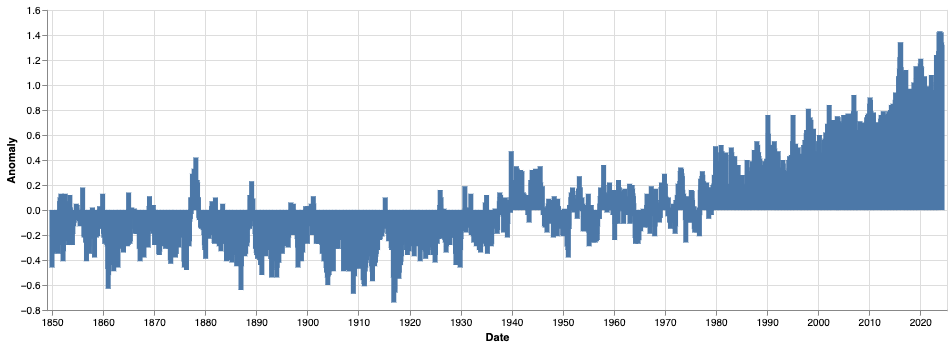
Now, change the color by setting the color channel. Use the color scheme attribute to set the color scheme. Set also the reverse attribute to invert colors and associate the red tonalities with hotter temperatures and the blue tonalities with colder ones.
chart = alt.Chart(df
).mark_bar(
).encode(
    x='Date',
    y='Anomaly',
    color=alt.Color('Anomaly', scale=alt.Scale(scheme='redblue', reverse=True))
).properties(
    width=800
)

chart
The following figure shows the resulting chart:

The problem now is that many bars overlap and are not shown correctly. One possible solution could be extending the chart width or reducing the bar size. Another solution involves grouping data by decades. Let’s apply this last solution: group data by decades and remove the last decade (2020s), which is incomplete. Use the Altair functions associated with transformations:
The following code shows how to implement the chart:
chart = alt.Chart(df
).mark_bar(
).encode(
    x='Decade:N',
    y='Anomaly',
    color=alt.Color('Anomaly', scale=alt.Scale(scheme='redblue', reverse=True))
).properties(
    width=800
).transform_filter(
    "year(datum.Date) < 2020"
).transform_calculate(
     Decade = "(year(datum.Date) - year(datum.Date) % 10)"  # Calculate the decade
).transform_aggregate(
    Anomaly='mean(Anomaly)',
    groupby=['Decade']
)

chart
The following figure shows the resulting chart:

Now we can adjust axes, by setting the title of the y-axis and rotating the x-axis labels:
chart = chart.encode(
    x=alt.X('Decade:O', axis=alt.Axis(
        title='',
        labelAngle=0,
        labelExpr="datum.value + 's'",  # Add 's' to the end of each decade label
        )
    ),
    y=alt.Y('Anomaly', title='Global Surface Temperature Anomalies (°C)'),
    color=alt.Color('Anomaly', scale=alt.Scale(scheme='redblue', reverse=True))
)

chart
Here is the resulting chart:

We have completed the basic chart. Now, we can add details specific to our professional audience, such as the values for each bar.
Let’s use the mark_text() function to add the label for each bar:
text = chart.mark_text(
    align='center',
    baseline='top',
    dy = alt.expr(alt.expr.if_(alt.datum.Anomaly > 0, -15, 5))
).encode(
    text=alt.Text('mean(Anomaly):Q', format='.2f'),  # Format the anomaly value with 2 decimal places

)

chart + text
Also, adjust the y-axis ranges to make the labels more visible.
The following chart shows the resulting chart:

Other useful information that our audience could want to extract from the chart are:
Let’s add the first as the subtitle of the chart, as shown in the following code:
chart = chart.properties(
    title=alt.TitleParams(
        text='Global Surface Temperature Anomalies',
        subtitle='Between the 1850s and the 2010s, surface temperatures increased by 0.94°C.',
    )
)

chart + text
Let’s add the second as a reference vertical line in correspondence of 1977 when the temperatures started to increase:
# reference line

rl_df = pd.DataFrame({
    'x'     : [1970],
    'text'  : [['Since 1977 temperatures', 'slowly started to increase.']]
})

rl = alt.Chart(rl_df).mark_rule(
    color='red',
).encode(
    x='x:N'
)

text_rl = rl.mark_text(
    color = 'red',
    baseline='top',
    align='left',
    y=10,
    dx=10
).encode(
    text='text'
)

chart + text + rl + text_rl
Note that we have set the x value for the reference value to 1970, since the x-axis does not contain 1977, but to be more specific, we have added a text which specifies the exact year (1977). The following figure shows the resulting chart:
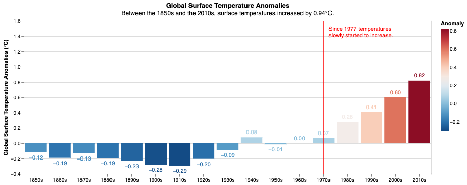
What do we want our audience of professionals to do? Possible answers to this question include:
Let’s focus on predicting future trends and assume we want to encourage our audience to start working on predictions. In correspondence, for example, we can add a new bar to the chart, representing a black box of the 2050s with a question mark as a label. This should encourage our audience to do the analysis.
To implement the chart, perform the following operations:
The following code implements the described steps:
pred_df = pd.DataFrame({
    'x'     : ['2050'],
    'y'     : [1.2],
    'text'  :  '?'
})

pred =  alt.Chart(pred_df
).mark_bar(
    color = 'black'
).encode(
    x = 'x:N',
    y = 'y'
)

pred_text = pred.mark_text(
    color = 'black',
    dy=-15
).encode(
    text = 'text'
)

chart = chart.properties(
    title=alt.TitleParams(
        text='How big will the temperature anomaly be in 2050?',
        subtitle='Between the 1850s and the 2010s, surface temperatures increased by 0.94°C.'
    )
)

final = (chart + text + rl + text_rl + pred + pred_text)
final
The following figure shows the resulting chart:
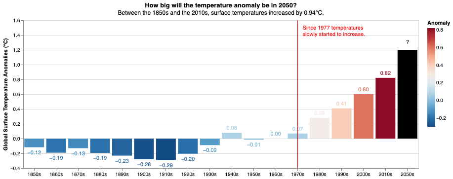
Now, you are ready to show your chart to your audience of professionals!
In this tutorial, you have learned how to tailor a chart to an audience of professionals. Professionals are technical people who aim to understand data, so they want numbers.
Do the math for them and answer their possible questions. Also, invite them to perform some kind of next step, such as further analysis.
You can find the code of this tutorial in this GitHub repository.
You can also watch the tutorial at the following link:
If you have reached so far in the reading, for me, today, it’s enough! Thanks, and see you next time!
If you want to increase the title font size, use the following command:
final.configure_title(
    fontSize = 30,
    subtitleFontSize= 20
)
How to Tailor a Chart to an Audience of Professionals was originally published in Towards Data Science on Medium, where people are continuing the conversation by highlighting and responding to this story.
Originally appeared here:
How to Tailor a Chart to an Audience of Professionals
Go Here to Read this Fast! How to Tailor a Chart to an Audience of Professionals